Article

Quantifying the Spatio-Temporal Variations and Impacts of Factors on Vegetation Water Use Efficiency Using STL Decomposition and Geodetector Method

1
Faculty of Geomatics, Lanzhou Jiaotong University, Lanzhou 730070, China
2
National-Local Joint Engineering Research Center of Technologies and Applications for National Geographic State Monitoring, Lanzhou 730070, China
3
Gansu Academy of Eco-Environmental Sciences, Lanzhou 730030, China
*
Author to whom correspondence should be addressed.
Remote Sens. 2022, 14(23), 5926; https://doi.org/10.3390/rs14235926
Submission received: 28 September 2022 / Revised: 5 November 2022 / Accepted: 14 November 2022 / Published: 23 November 2022
(This article belongs to the Section Remote Sensing in Agriculture and Vegetation)

Abstract

:
Water use efficiency of vegetation (WUE), the ratio of carbon gain to water loss, is a valid indicator to describe the photosynthetic carbon–water coupling relationship. Understanding how and why WUE changes are essential for regional ecological conservation. However, the impacts of various factors and their interactions on the spatial variation of WUE remain uncertain in the arid land of Northwest China. Here, we selected the Qilian Mountains (QM) and Hexi Corridor (HC) as the study areas. Supported by the Google Earth Engine, we explored the spatio-temporal variations of WUE in QM and HC for 2002–2021 using STL decomposition (a seasonal-trend decomposition procedure), trend analysis, and the Hurst index. Then, the Geodetector method was applied to quantify impacts of geographical and eco-meteorological factors on the spatial variation of WUE. The WUE in HC was higher than that in QM. Interestingly, the opposite longitude zonality characteristics are shown in the QM and HC. In QM, the WUE showed an upward trend with longitude increasing, while a downward trend with longitude increasing in the oases of HC. The WUE of cropland was the highest (1.15 ± 0.35 gC kg−1 H2O), and that of alpine vegetation was the lowest (0.2 ± 0.15 gC kg−1 H2O). WUE showed a decreasing trend across the study area, almost certainly due to a drop from May to July during 2002–2021. The air temperature is the dominant factor influencing the spatial variation of WUE. In addition, the interaction of any two factors is greater than the independent influence of either factor alone. The Geodetector method proved to be effective for quantifying the impact of complex multi-factors on the spatial variation of WUE. This study provides a new technical scheme to analyze the spatio-temporal pattern and quantify the impact of multi-factors on the spatial variation of WUE. These findings aid in understanding underlying mechanisms of WUE variation and thereby will be beneficial for clarifying the response of vegetation to climate change.

Graphical Abstract

1. Introduction

Climate change impacts significantly on the structure and function of terrestrial ecosystems [1,2]. Against this background, interactions between the water and carbon cycles have received increasing attention. Vegetation water use efficiency (WUE), defined as the ratio of gross primary productivity (GPP) and evapotranspiration (ET), is one of the most direct indicators of water–carbon coupling [3]. Studying the spatial and temporal changes in WUE helps us understand the coupling relationship between water and carbon in vegetation and further deepens our understanding of the impact of climate change on vegetation.
The feedback mechanism between climate change and the water–carbon cycle of ecosystems is extremely intricate. Traditional biomass growth surveys and the study of eco-hydrological processes are not suitable for short-term analysis because of consuming time and lack of precision [3]. New techniques, such as the eddy covariance method, can improve these studies. The eddy covariance method, a micro-meteorological technique, could directly measure the transport of carbon and water on a time scale of seconds [4]. Nevertheless, the observations are limited to the adjacent region and are unsuitable for macroscopic monitoring [5].
Remote sensing (RS) offers an excellent technological tool for WUE research. Extensive research has shown that the quantitative retrieval of WUE based on RS data allows for the continuous monitoring of WUE over a vast area [6,7,8]. These studies focused on the RS estimation of WUE [7,9], the spatial distribution pattern and change tracking [10,11], the response of WUE to climate change and its sensitivity [12,13], and the effect of land cover change on WUE [14]. Compared with other high temporal resolution satellite data, such as Advanced Very High Resolution Radiometer (AVHRR), SPOT VEGETATION, and HuanJing-1B, Moderate Resolution Imaging Spectroradiometer (MODIS) provided extensive quantitative RS products. In addition, Landsat imagery with high spatial resolution suffered from a lack of data due to the long acquisition cycle and cloud coverage compared to MODIS datasets [15], making it difficult to monitor WUE changes accurately. MODIS datasets are currently the most suitable data for monitoring WUE [5,11] and understanding vegetation responses to climate change [11]. Given this, we utilized MODIS GPP and ET products to examine WUE variations.
Previous studies have focused on the spatio-temporal trend of WUE and have shown that the global WUE exhibited a general upward trend but with significant spatial heterogeneity [11,16,17]. Although a general linear regression model can estimate the average growth rate, cyclical variation is retained in the residuals, thus leading to a bias of model uncertainty [18]. The process of WUE change over time cannot be clearly shown. As illustrated in Figure 1, the inter-annual trend may be influenced by seasonal oscillations, which obscure long-term trends. The STL decomposition method is a seasonal-trend decomposition procedure that allows fast computation due to a simple design that comprises a sequence of loss smoothers and robustly estimates the trend and seasonal components that are not distorted by outliers [19]. Thus, this method has been used successfully to analyze time series for leaf area index (LAI) [20], normalized difference vegetation index (NDVI) [18], and chlorophyll-a [21], but not for the WUE time series before this study.
Recently, an increasing number of studies have analyzed the relationship between bio-climatic conditions and WUE temporal trend [13]. For example, Li et al. [22] used multiple linear regression analysis to examine the response of regionally averaged WUE to temperature, precipitation, and LAI in China. However, the WUE change is complex and driven by various factors. The relationship between WUE variation and each factor cannot be described by a simple linear equation. The influence of various factors and their interactions on the spatial variation of WUE is still uncertain. Previous studies have shown that the temporal trend in WUE was influenced by a combination of factors [23,24,25,26], such as climate factors, LAI, soil moisture, vegetation cover, and phenology, but factors influencing the temporal variation in WUE may differ from those influencing spatial variation [17]. The research to date has tended to focus on the influence of different factors on WUE temporal variation rather than on spatial variation. Therefore, it is challenging to detect the effects of various factors and their interactions on the spatial variation of WUE. Geodetector, a spatial analysis method, could detect the linear and non-linear relationships between the dependent variable and its explanatory variables and could quantitatively capture the impact of different factors on spatial heterogeneity [27]. A major advantage of the Geodetector method is that it overcomes the limitations of traditional statistical methods that cannot handle category variables. Hence, this method may be a valid tool to differentiate the drivers of WUE spatial variation in arid lands of Northwest China.
In recent years, the development of cloud computing has substantially improved the processing capability of RS big data. For example, Google Earth Engine (GEE) can provide planetary-scale geospatial analysis based on its advanced cloud computing and storage capability [28] and has been widely used in land cover mapping [29], crop yield estimation [30], global water monitoring [31], etc. GEE offers a platform for investigating the spatio-temporal variation of WUE over a long period at the local, regional, or even global scale.
To understand the impacts of various factors and their interactions on the spatial variation of WUE in the arid land of Northwest China, we selected the Qilian Mountains (QM) and Hexi Corridor (HC) as the study areas, a typical arid land environment with mountains, oases, and deserts. The QM and HC regions are located in the middle of Northwest China with complex topography. The vegetation status of the QM and HC is critical to the ecological security in Northwest China. Recently, studies on vegetation RS monitoring in this region have mainly focused on vegetation phenology [32], vegetation index [33,34], vegetation cover [35,36], biomass [37,38], and GPP [39,40]. WUE was rarely concerned. In recent years, the vegetation status in this region has experienced obvious changes in response to climate change, and a thorough investigation of changes in its WUE of vegetation is needed.
As discussed above, this study aims to (1) investigate the spatio-temporal variations of WUE in QM and HC from 2002 to 2021, based on the GEE platform, using MODIS products and the STL decomposition method, and (2) quantify the influence of potential factors (climate, topography, and ecological factors) and their interactions on the spatial heterogeneity of WUE, based on the Geodetector method. The study results will help to protect the ecological environment, and further understand the underlying mechanisms of WUE changes in the arid land of Northwest China.

2. Materials and Methods

2.1. Study Area

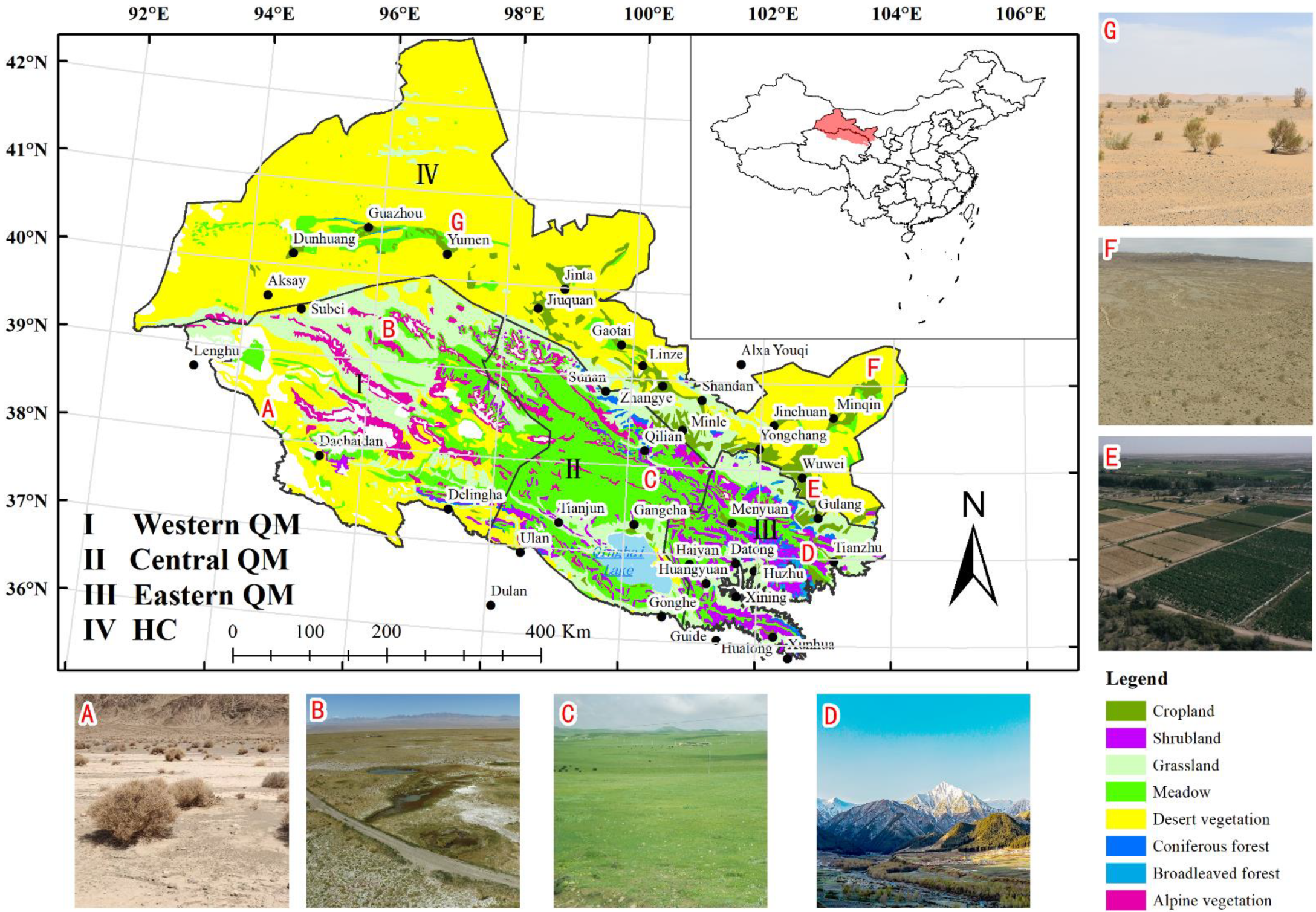
Mountains, oases, and deserts constitute a unique triadic coupling system in the arid lands of Northwest China. Snow and glaciers in the mountains provide water for numerous streams in the valleys, which nourish the oasis and desert vegetation at the foot of the mountains. Mountains, oases, and deserts are linked as a whole through water. Given this, we selected the representative QM and HC regions in the arid lands of Northwest China for our study. Meanwhile, considering the topography, vegetation, and watershed distribution, we took the QM and HC regions as a whole and delineated the spatial scope of the study area (Figure 2).
The spatial extent of the study area is 93°30′–103°00′E and 35°43′–39°36′N. Located in the northeastern Tibetan Plateau, the QM is one of the alpine mountain systems in Northwest China, which runs from northwest to southeast and spans Qinghai and Gansu provinces. Most of the mountains are above 4000 m. The HC region, a narrow valley running northwest-southeast, is located in the northern Qilian Mountains, at an elevation of 1100 to 1700 m. The topography of the study area is complex, and there are significant differences in water and heat conditions, soil conditions, and vegetation cover [32]. The QM and HC regions are distinct natural geographic units connected by water resources. The QM region recharges numerous in-stream rivers, maintains the oasis and desert ecosystems in HC, and affects the local ecological environment.
The study area spans approximately 10° of longitude. The western part of the study area is governed by the westerly circulation, whereas the eastern is dominated by the southeast and southwest monsoons. The combined influence of the two circulation systems and the Tibetan Plateau monsoon in the central region results in a complicated local climate [37]. Accordingly, and in combination with previous studies [37], the study area was divided into four sub-areas: eastern QM, central QM, western QM, and HC, to investigate the regional differences in WUE (Figure 2).

2.2. Data Sources

The used RS data includes 8-day synthetic products of MOD16A2.006 (ET), MOD17A2H.006 (GPP), and MOD15A2H.061 (LAI) from the GEE geodatabase (https://developers.google.com/earth-engine, accessed on 12 May 2022) with a spatial resolution of 500 m and the period of 2002–2021. In a single year, 46 values were acquired. The data was evaluated by several regional ground observations and is widely used in regional or global scale studies [5,8,11,16]. ET, GPP, and LAI products contain data quality control layers (ET_QC, Psn_QC, and FparLai_QC), which record sensor information, cloud coverage, and quality reliability. In this study, we used GEE to accomplish data preprocessing.
The climate and soil moisture data were gathered from the National Tibetan Plateau Data Center (TPDC) (http://data.tpdc.ac.cn/en/, accessed on 15 August 2022). The climate data were extracted from the China meteorological forcing dataset (CMFD), which covers the period 1979–2018 with a spatial resolution of 0.1° [41,42]. The soil moisture data were derived from the Soil Moisture in China dataset (SMC). The period span is 2002–2018, and the spatial resolution is 0.05° [43].
The digital elevation model (DEM) data used were the SRTM DEM acquired by INSAR technology with two spatial resolutions of 30 m (SRTM1) and 90 m (SRTM3). We used SRTM3 (data revision V4) to calculate the slope, aspect, slope position, and topographic position index (TPI) [44]. Table 1 details the data used in this paper.

2.3. Methods

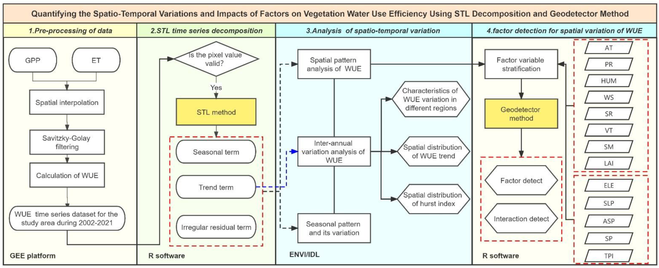
Figure 3 shows the technical scheme, including four key steps: (1) data preprocessing, (2) STL time series decomposition, (3) analysis of the spatio-temporal variations of WUE, and (4) factor detection for the spatial pattern of WUE.

2.3.1. Data Preprocessing

WUE was calculated with an 8-day time interval and 500 m spatial resolution during 2002–2021 using MODIS ET (MOD16A2.006) and MODIS GPP (MOD17A2H.006) products on the GEE platform. The monthly WUE was the average of the WUE at 8-day intervals throughout the month. If an 8-day synthetic data value occurred in two consecutive months, it was credited to the month in which more days appeared during those eight days. Similarly, the annual average WUE was determined. The WUE calculation formula was shown as follows:
W U E = G P P / E T
To address the problems of missing data and accuracy degradation of GPP and ET time series caused by cloud contamination, precipitation, snowfall, and sensor errors, we performed spatial interpolation and temporal filtering smoothing of GPP and ET time series using the inverse distance weight interpolation method and the S-G filter method, respectively. The S-G filter method is a least-squares local filtering method without strict restrictions on the sensor type [45]. The reconstructed data was of higher quality and was widely used for data smoothing and noise reduction.

2.3.2. STL Decomposition

The cyclical season pattern caused by the Earth’s orbit around the Sun “carved names” on many ecological and environmental time series. This annual seasonal oscillation must first be distinguished to comprehend the time series change [21,46]. The STL decomposition method is a nonparametric statistical method proposed by [19]. It comprises two main components: an inner loop for fitting the trend and period terms and an outer loop for calculating robustness weights to reduce the effects of outliers. The basic formula was shown as follows:
W U E t = T t + S t + R t
where WUEt is the value observed at time t. Tt, St, and Rt represent the trend term, the seasonal term, and the irregular residual term, respectively. Tt contains long-term and non-periodic trend signals, such as long-term trends caused by climate change. St refers to the seasonal pattern caused by the Earth’s revolution. Rt involves other residuals that cannot be explained by trends or seasonal effects.
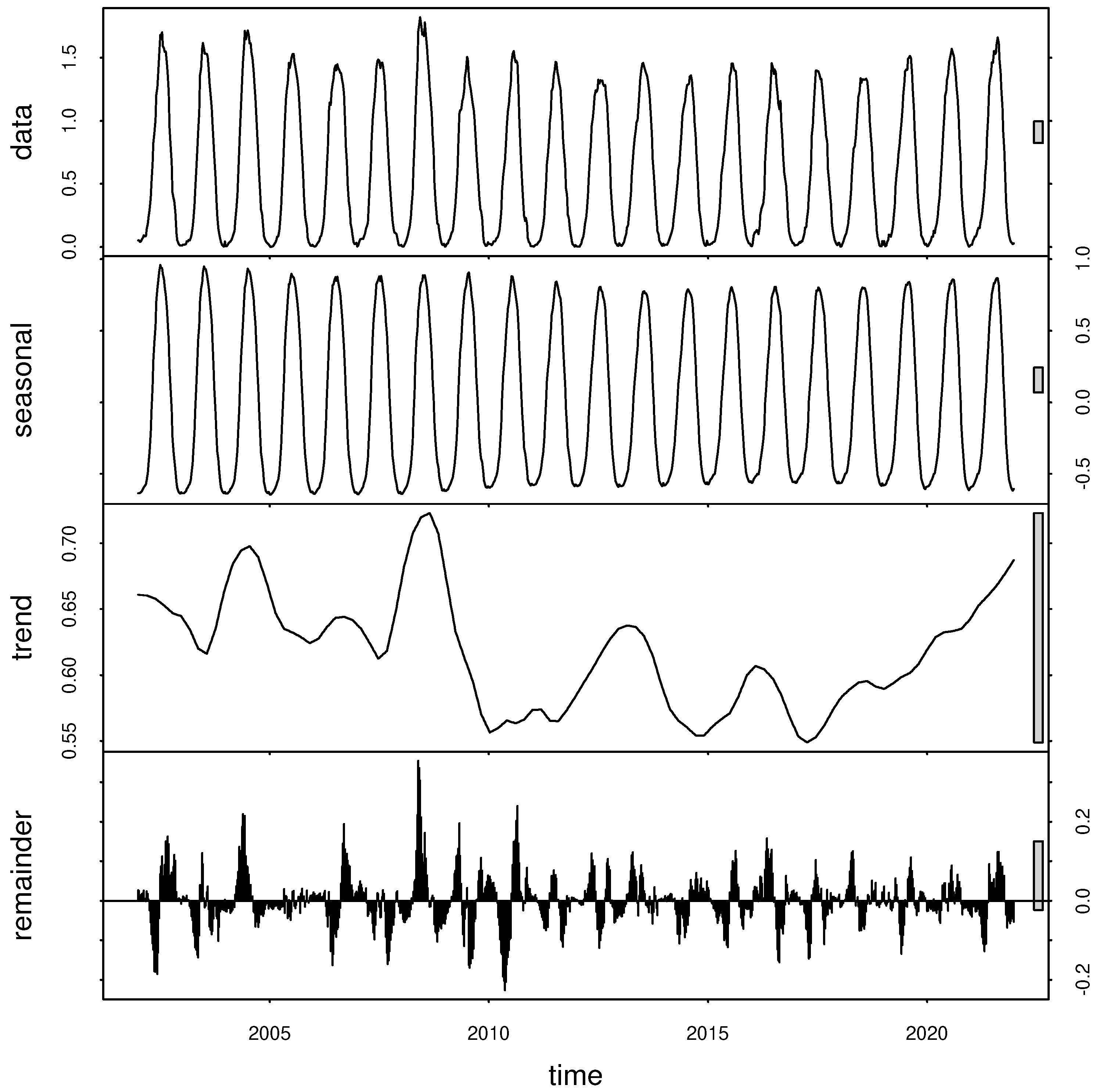
WUE time series have trend and periodicity characteristics. Decomposing the time series can more clearly reveal the variation patterns of WUE. The STL seasonal decomposition method was used to mine the information inherent in the time series of WUE. We implemented the STL decomposition pixel-by-pixel programmatically using the terra and forecast packages in R [47]. The starting date of the time series was set to 2002–01, and the ending date was set to 2021–46. All parameters in the STL seasonal decomposition process were determined automatically except for the robust parameter, which controls whether a robust fit was used in the locally weighted regression. The robust parameter was set to FALSE because the WUE time series had been smoothed by the S-G filtering beforehand. Figure 4 depicts an example of WUE time series decomposition using the STL method for a grassland pixel from 2002 to 2021.

2.3.3. Analysis Method of Spatio-Temporal Variation Characteristics

The Sen trend degree (β) was used to analyze the WUE trend from 2002 to 2021. The β was determined using the following formula:
β = median x j x i j i
where 1 < j < i < n. When β > 0, it means that the time series is increasing. When β < 0, it means that the time series is decreasing. However, β can only reflect the magnitude of the trend, and the significance of the changing trend cannot be determined by itself. Therefore, the nonparametric Mann–Kendall (M-K) test method [48] was used to determine the statistical significance of each pixel’s trend.
We used the Hurst index, as described in Rivas-Tabares et al. [49], to quantify the sustainability of the WUE time series. The Hurst index includes three forms. When 0.5 < H < 1, it means that the time series had sustainability. When 0 < H < 0.5, it means that the time series had inverse sustainability, i.e., the future trend of the series is opposite to its past trend. Furthermore, when H = 0.5, it refers that the series has the characteristic of random wandering.

2.3.4. Factor Detection for Spatial Variation of WUE

If a dependent variable is influenced by an independent variable, the spatial distributions of the dependent and independent variables should be consistent. Based on the theory of spatial stratified heterogeneity, Wang et al. [27,50] proposed a novel statistical method, Geodetector, to measure the correlation between the independent and dependent variables. The Geodetector method overcomes the limits of classic statistical methods when handling categorical variables and can detect the linear and nonlinear relationships between two certain variables. It is applicable to quantitative attribution analysis for spatial patterns of geographic variables [51,52,53]. The Geodetector method includes four detectors. In this paper, 2 detectors, i.e., the factor detector and interaction detector, were used.
  • Factor detector
The factor detector measures the degree to which a certain factor explains the spatial heterogeneity of the dependent variable using the q value (Equation (4)),
q = 1 h = 1 L N h σ h 2 N σ 2
where h is the partition of a certain factor X or the dependent variable Y. Here, X represents 13 factors (AT, PR, HUM, WS, SR, VT, LAI, SM, ELE, SLP, ASP, SP, and TPI). Y refers to WUE. Nh and N are the number of units in partition h and the entire region, respectively. The σ h 2 and σ2 are the variances in partition h and the entire region, respectively. The q value shows the magnitude of the explanatory power of X to Y with a range of 0 to 1. The larger the q value, the stronger the explanatory power.
A simple transformation of the q value satisfied the noncentral F distribution with the 1st df L-1, the 2nd df N-L, and non-centrality λ [54].
F = N L L 1 × q 1 q ~ F ( L 1 , N L ; λ )
The significance of the q value can be tested by looking up the F-distribution table.
2.
Interaction detector
The interaction detector estimates whether the interaction of any two factors (X1 and X2) enhances or weakens their explanatory power on the dependent variable Y [55]. First, the q value of X1 and X2 on Y was calculated separately (q(X1) and q(X2)). Then, the q value of the interaction, q(X1∩X2), was calculated. Finally, the values of q(X1), q(X2), and q(X1X2) were compared to show the type of interaction between the two factors [56].
We use the GD package in R, which was developed by Song et al. [57], to implement the Geodetector method.

3. Results

3.1. Spatial Distribution of WUE

The annual average WUE was 0.60 ± 0.36 gC kg−1 H2O during 2002–2021 in the study area (pixels with a NULL value in the desert and Gobi were not included in the statistics). The WUE showed obvious spatial heterogeneity (Figure 5). The annual average WUE tended to increase from west to east, ranging from 0.01 to 2.63 gC kg−1 H2O. Higher values of WUE occurred in relatively humid areas, such as the eastern QM and the oases of HC. In arid and sparsely vegetated areas, such as the western QM, WUE was low. The spatial pattern of WUE in spring and fall is similar to the spatial pattern of the annual average WUE.
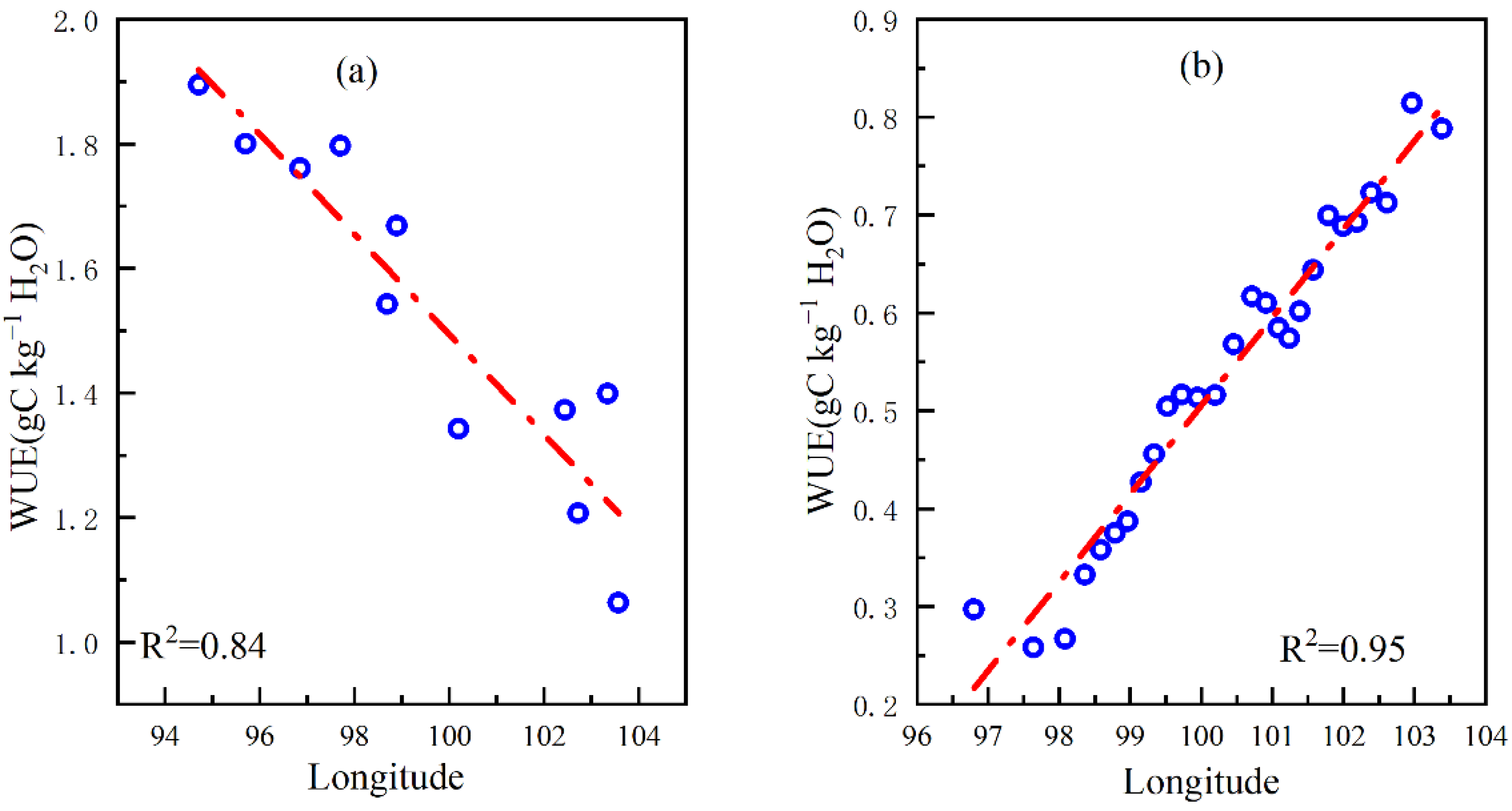
It was further investigated by two major geographical units, the QM and HC regions. The WUE in the QM showed obvious longitude zonality with an eastward-increasing tendency. In the western, central, and eastern QM, the multi-year average WUE was 0.28, 0.47, and 0.70 gC kg−1 H2O, respectively. While the distribution of WUE in the oases within the HC was exactly the opposite, showing an eastward-decreasing trend. The average WUE in the HC was 1.09 ± 0.34 gC kg−1 H2O, with significant spatial variations. The annual average WUE value was the lowest in Dajing Oasis at the eastern end of HC, while it was the highest in Dunhuang Oasis at the western end of the HC. The WUE of Dunhuang Oasis was approximately 79% greater than that of Dajing Oasis.
The oases of HC were ranked by their annual average WUE in the following order:
Dunhuang Oasis (1.90) > Guazhou Oasis (1.80) > Huahai Oasis (1.79) > Yumen Oasis (1.76) > Jinta Oasis (1.66) > Jiuquan Oasis (1.54) > Minqin Oasis (1.39) > Jinchang Oasis (1.37) > Zhangye Oasis (1.34) > Wuwei Oasis (1.21) > Dajing Oasis (1.06). The unit for the numbers in parentheses is gC kg−1 H2O.
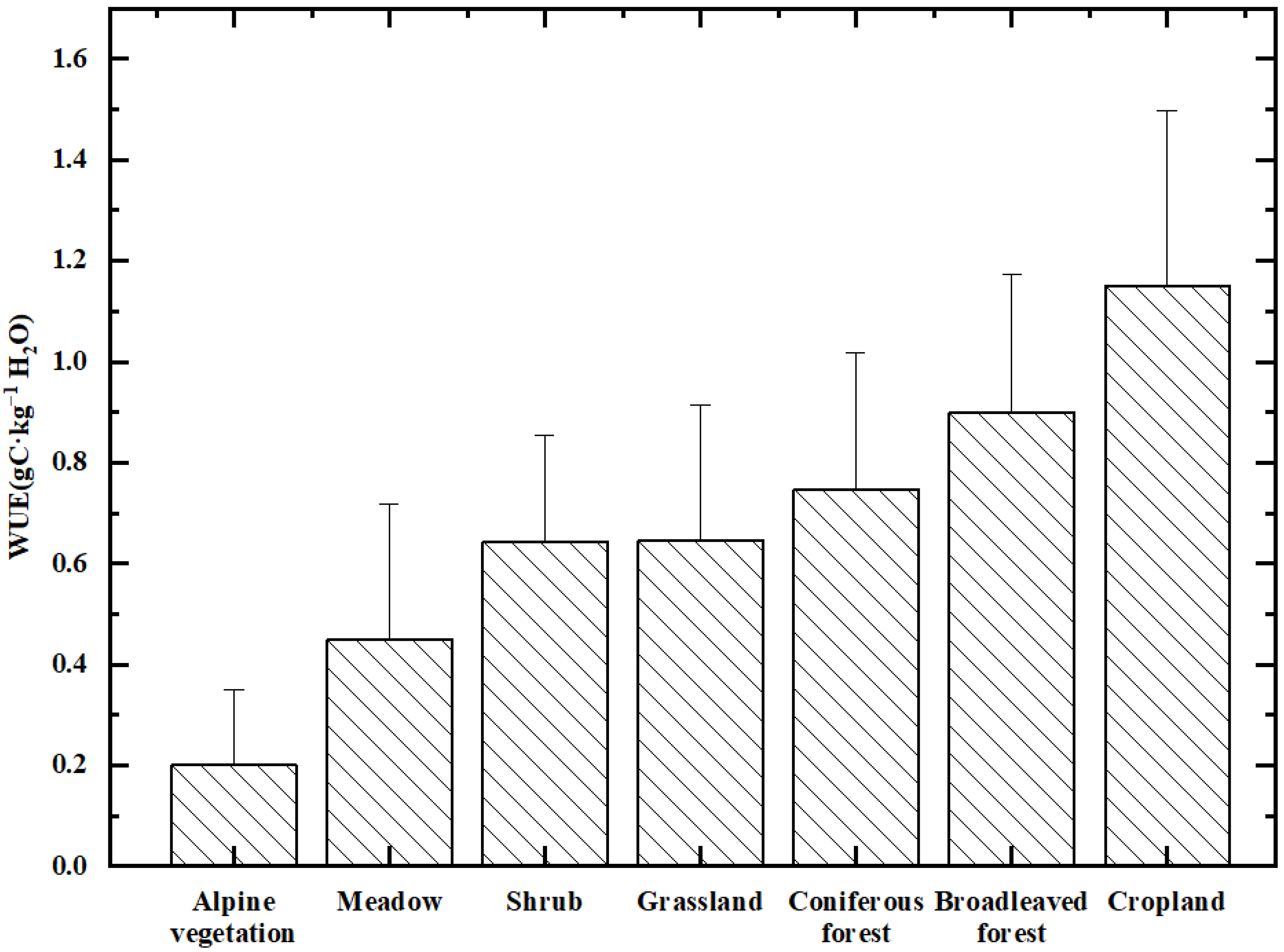
The average annual WUE was overlaid with a vegetation-type map to obtain the WUE characteristics for each vegetation type within the study area. During 2002–2021, the average WUE of the seven vegetation types ranged from 0.2 to 1.15 gC kg−1 H2O (Figure 6), with the highest WUE (1.15 gC kg−1 H2O) for cropland, followed by broadleaved and coniferous forests with 0.90 and 0.75 gC kg−1 H2O, respectively. Grassland, shrubs, meadows, and alpine vegetation followed in that order. Overall, the WUE of woodlands was significantly higher than that of shrubs and herbaceous plants, except for cropland affected by human activities.

3.2. Inter-Annual Variation of WUE

The WUE time series at the 8-day interval scale from 2002 to 2021 was decomposed using the STL decomposition method into three components: the trend term, the seasonal term, and the stochastic fluctuation term (Figure 7). The trend term was centered on its mean value to facilitate the observation and comparison of the three components. According to the trend term, the WUE displayed a fluctuating decreasing trend from 2002 to 2021. WUE varied between 0.53–0.71 gC kg−1 H2O and decreased at an average rate of 0.002 gC kg−1 H2O/a. The change in WUE can be divided into three time stages to discuss its inter-annual variation pattern. From 2002 to 2010, WUE fluctuated at a relatively high level, reaching two peaks in 2004 and 2009 at 0.69 and 0.71 gC kg−1 H2O, respectively. From 2010 to 2017, WUE fluctuated at a relatively low level, reaching peaks in 2013 and 2016, respectively. During the period 2017–2021, WUE increased continuously from 0.53 gC kg−1 H2O to 0.68 gC kg−1 H2O.
According to the results of the Mann–Kendall test (Table 2), the results show that the p-value for each zone was close to zero (<0.01). Combining the Z value, it can be found that the WUE in each zone showed a significantly decreasing trend at a 0.01 confidence level.
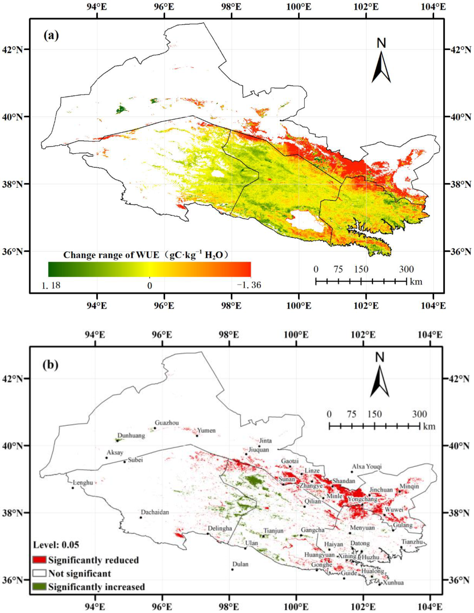
We used the Sen method to investigate the spatial heterogeneity of the WUE change by analyzing the trend term of WUE time series. The spatial distribution of WUE change magnitude and the significance test results were calculated (Figure 8). The area with a valid WUE value was analyzed, excluding the non-vegetated regions such as deserts, Gobi, and glaciers. The magnitude of WUE change ranged from −1.36 to 1.18 gC kg−1 H2O over the last 20 years. The proportion with positive change was 37%, while that with negative change was 63%. WUE decreased significantly in the eastern and central HC and the surroundings of Qinghai Lake. Furthermore, the significant increase in WUE was concentrated in central QM. The WUE in Dunhuang and Guazhou Oasis, located in the western HC, also showed an upward trend. Statistical analysis was conducted based on the results of the Sen trend and the M-K test (Table 3). The results show that the percentage of slightly and significantly improved areas was 6.4%, while the percentage of slightly and severely degraded areas was 18.2%.
The average Hurst index in the WUE of the whole study area reached 0.72. The area with a Hurst index of less than 0.4 accounted for a minor proportion (0.4%) and was mainly located in the central QM, from Hala Lake to Qinghai Lake and Qilian County. WUE there will change from the current upward trend to a downward trend in the future, showing a strong anti-continuity. The area with a Hurst index greater than 0.6 was primarily located in the eastern QM, the HC oases, the surroundings of Qinghai Lake, and the west of Hala Lake, accounting for 32.4%. WUE showed strong continuity in the future.

3.3. Seasonal Pattern of WUE

The intra-annual variation of WUE was approximately a bell curve. In November, December, and January, the WUE was low with an average of 0.025 gC kg−1 H2O due to the low temperature and inactive plant photosynthesis. From February to June, the WUE increased dramatically because of the enhanced solar radiation and suitable water and heat conditions. As the air temperature declined and plant photosynthesis reduced from July to October, vegetation growth entered the declining phase and WUE decreased significantly. Throughout the growing season (April to October), the WUE ranged from 0.23 to 1.48 gC kg−1 H2O. The highest value was recorded in the 26th 8-day period (201st to 208th day of one year).
Influenced by vegetation physiological and ecological characteristics of vegetation, different vegetation types showed distinct seasonal patterns (Figure 9). The WUE of cropland showed an approximate bimodal pattern, peaking in the 18th and 31st 8-day periods, respectively. The first peak was considerably higher than the second. Other vegetation types showed a single-peaked pattern, with the peak in early July. The peak value was ranked as follows: cropland > broadleaved forest > coniferous forest > shrub > grassland > meadow > alpine vegetation.

3.4. Influence of Geographical Factors on the Spatial Variation of WUE

First, we investigated the relationship between longitude and WUE in HC and QM, respectively. It showed a negative relationship (R2 = 0.95) between longitude and WUE in HC. While in contrast, a significant positive relationship (R2 = 0.84) existed between longitude and WUE in the QM (Figure 10). In HC, the WUE decreased from west to east, while it showed a reverse scenario in QM. Its distribution pattern is consistent with that of temperature.
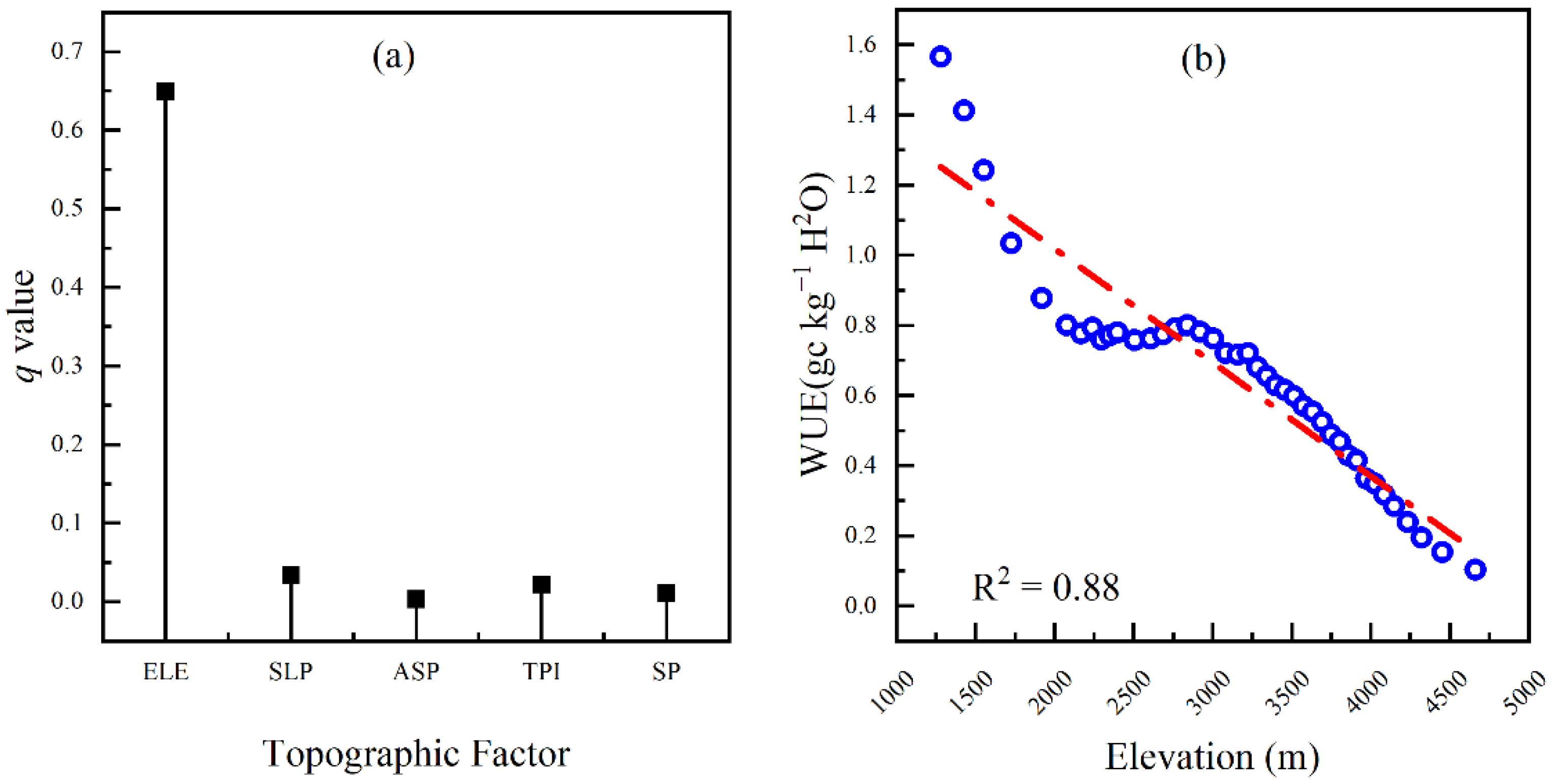
In addition, we also explored the relationships between topographic factors and WUE using the Geodetector method (Figure 11a). It was found that elevation was the key topographic factor contributing to the spatial heterogeneity of WUE, while slope, aspect, TPI, and slope position were less influential. Further analysis of the relationship between elevation and WUE (Figure 11b) revealed that WUE showed a negative relationship with the elevation gradient. WUE tended to decrease with increasing elevation, which may have resulted from changing climatic conditions due to the elevation gradient [58].

3.5. Impact of Bio-Meteorological Factors on the Spatial Variation of WUE

Factor detection showed that all eight bio-meteorological factors (AT, PR, HUM, WS, SR, VT, SM, and LAI) had a significant impact on the spatial variation of WUE (p < 0.01). As far as the whole study area is concerned, the impact of temperature on the spatial variation of WUE was the largest, and the explanatory power was up to 66.1%. The following factors, in order, were specific humidity, vegetation type, and LAI, with an explanatory power of 52.6%, 34.2%, and 29.6%, respectively. Shortwave radiation, precipitation, and wind speed explained only 17.3%, 16.6%, and 16.2%, respectively. The explanatory power of soil moisture was the lowest (5%).
However, the explanatory power of factors for the spatial variation of WUE varied somewhat across regions (Figure 12). For example, the explanatory power of shortwave radiation varied considerably in different zones. It was 7.5% in the eastern QM, whereas as high as 30.9% in the western QM. In terms of precipitation, its explanatory power was stronger in desert regions with arid climates, such as the western QM and HC. Nevertheless, it was weaker in the relatively humid eastern and central QM (only 6.3% in the central QM). The explanatory power of LAI was close in different zones, with q values ranging from 0.169 to 0.376 and was the weakest in western QM where vegetation is sparse. The explanatory power of temperature was higher than other bio-meteorological factors. It reached over 42% in all sub-areas and even up to 59.3% in HC Oases.
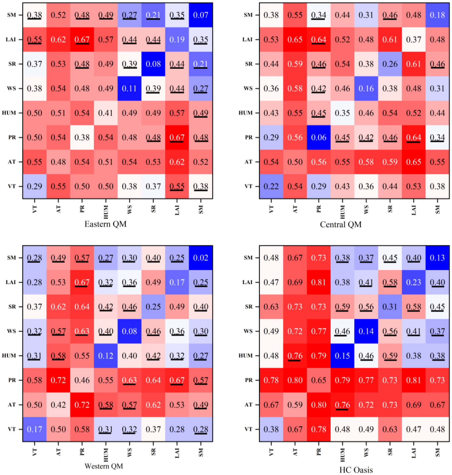
An interaction detector was used to assess the explanatory power of factor interactions on the spatial variation of WUE (Figure 13). If the q value of the two-factor interaction is greater than the maximum of the q values of factors X1 and X2 but less than the sum of both, it implies that the two factors are mutually enhanced. If the q value of the two-factor interaction is greater than the sum of the q values of X1 and X2, the two factors are non-linearly enhanced. The results of this paper showed that the q value of any two-factor interaction on the spatial variation of WUE was greater than that of a single factor, which means that the explanatory power of a single factor could be enhanced when interacting with others. The interaction of the two factors on the spatial variation of WUE was greater than the impact of either factor acting alone. In 35% of the cases, the q values of the two-factor interaction were higher than the total q values of the two single factors, which showed that the two-factor interaction was non-linearly enhanced.
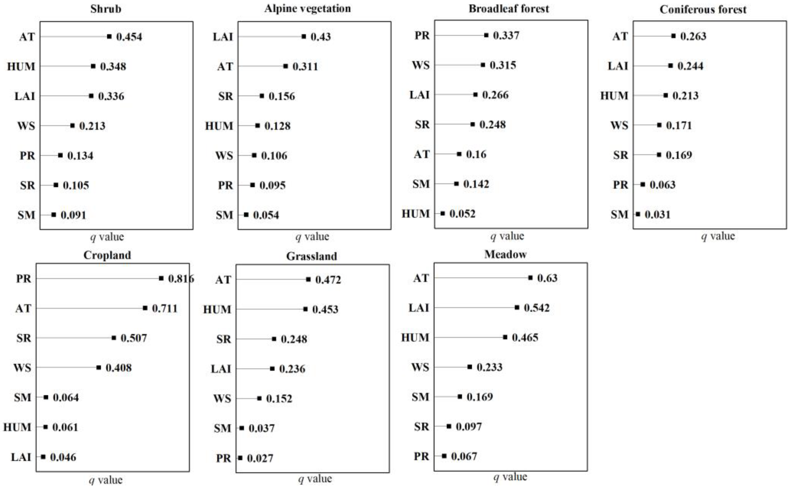
The impact of various bio-meteorological factors on the WUE of different vegetation types was investigated using the Geodetector method (Figure 14). The magnitude of the impact of bio-meteorological factors on WUE varied with vegetation type. It was found, however, that temperature was the most critical factor for most vegetation types.

4. Discussion

4.1. Spatio-Temporal Variations of WUE

This paper used MODIS ET and GPP products to estimate WUE in QM and HC. The spatial variation of WUE ranged from 0.01 to 2.63 gC kg−1 H2O. The average of WUE was 0.60 ± 0.36 gC kg−1 H2O during 2001–2021, lower than the global WUE average of 1.89 gC kg−1 H2O and 1.71 gC kg−1 H2O calculated by flux and RS, respectively [4]. The multi-year average of WUE in HC (1.09 ± 0.34 gC kg−1 H2O) was lower than that in Central Asia (2.56 gC kg−1 H2O) [59], also an arid desert region. It may be associated with the fact that cultivated vegetation predominates in HC [60]. Compared with Central Asia, the WUE in HC was more impacted by human activities, such as fertilization and irrigation [34,61]. The multi-year average WUE in QM was 0.5 ± 0.327 gC kg−1 H2O, lower than the average WUE (1.14 gC kg−1 H2O) calculated by Ji et al. [62] using MODIS data for grassland across the Tibetan Plateau and closer to the WUE of 0.4–1.38 gC kg−1 H2O using data from three flux towers in the Tibetan Plateau during 2003–2006 [63].
This study found an overall downward trend in WUE over the last 20 years in the study area. While an increase in atmospheric CO2 concentration led to an increase in temperature and WUE [64], excessive temperature also suppressed photosynthesis and promoted evaporation, which ultimately led to a decrease in WUE [65]. It differed from the study of WUE for grassland on the Tibetan Plateau [62], mainly due to the different spatial extent and periods. Our spatial extent, including QM and HC, differs from that of the Tibetan Plateau, although QM is a part of the Tibetan Plateau. In addition, the period was slightly different.
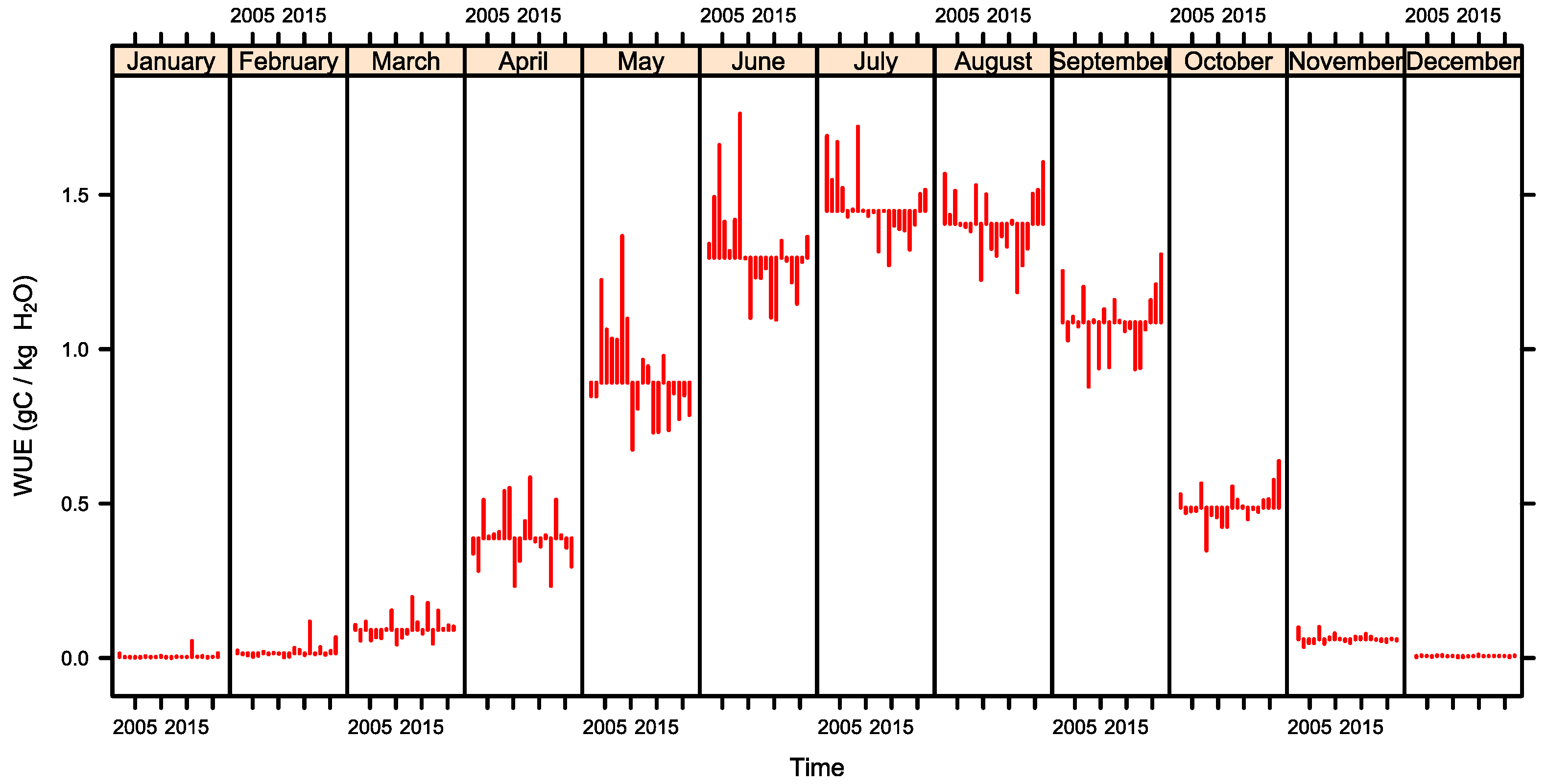
A monthly plot was used to investigate the seasonal pattern shift of WUE from 2002 to 2021 (Figure 15). The monthly plots represent the 12 monthly subseries of the WUE for each year from 2002 to 2021. The subseries fluctuates around the monthly mean. The monthly plots illustrate the long-term trends of the WUE for each month. We found an intriguing variation in the seasonal pattern: WUE tended to decrease from May to July (the early and mid-growing seasons), while the trend reversed to a slight increase from September to October (late growing season). It is almost certain that the reduction in WUE resulted from the reduction in WUE from May to July. This phenomenon may be due to changes in vegetation phenology and temperature [26]. In the early and middle of the growing season, GPP and ET showed an increasing trend due to higher temperature and earlier phenology [32,66]. Still, ET increased faster than GPP, resulting in a decreasing trend in WUE. In the late growing season, the delay in phenology kept WUE at a relatively high level, and WUE showed a slightly increasing trend. The regularity of seasonal pattern shift contradicts that in the northern hemisphere [67] and Luanhe River Basin [68], the typical semi-arid region in China, which shows that the shift in the seasonal pattern of WUE differed across areas.

4.2. Factor Analysis for Spatial Variation of WUE

The results of factor detection and interaction detection were analyzed jointly. In all four sub-areas, temperature and its interaction with other factors show strong explanatory power. Temperature is the dominant factor in the spatial distribution of WUE. It is consistent with the previous study [62]. Nandy et al. [10] also found that temperature was the most crucial driver of forest WUE change in India. Moreover, precipitation, LAI, and specific humidity also have strong explanatory power, but exhibit significant spatial heterogeneity. In the eastern QM, the top three interactions in terms of explanatory power were PR∩LAI (0.67), AT∩LAI (0.62), and HUM∩LAI (0.57). In the central QM, the top three interactions were AT∩LAI (0.65), PR∩LAI (0.64), and SR∩LAI (0.61), in that order. Although the explanatory power of LAI is not great when acting alone, its combination with temperature and precipitation can enhance the explanatory power. It suggested that the effect of temperature and precipitation on the spatial variation of WUE may be achieved by changing LAI [58]. The explanatory power of precipitation is considerably greater in the sparsely vegetated and arid western QM and HC than that in the relatively humid eastern and central QM. Namely, precipitation shows a stronger effect on the spatial variation of WUE in arid lands compared to relatively humid areas. Interaction detection also further corroborated the above conclusions. The top three interactions in the western QM and HC are all precipitation related.

4.3. Validity, Limitations, and Future Work

Identifying and analyzing the temporal trends in historical observation is an essential aspect of ecological time series analysis. In terms of decomposing the WUE time series, the STL method can well decompose the WUE time series into inter-annual trend and seasonal components and detect a nonlinear change in long-term trends, which could not be accomplished by general linear regression models [19]. As shown by the residual terms in Figure 4 and Figure 7, the residuals are distributed around the mean, indicating that the method extracts credible information on the trend and seasonal terms. The STL method can handle the outliers in the WUE time series and achieve robust and accurate estimates of the trend and seasonal components. The trend component could reveal the process of WUE change over time to reduce the uncertainty of the WUE time series analysis [18]. The effectiveness of the STL decomposition technique has also been demonstrated in several research papers [18,20,21].
Our study illustrated the validity of the Geodetector method in identifying the influence factors responsible for the spatial variation of the WUE. Compared to traditional statistical methods, it can quantify the nonlinear effect of factors and the interaction of pair-wise factors on the spatial variation of WUE [69,70]. GD package in R, which realized an optimal parameter-based Geodetector method, could avoid tedious parameter setting and conduct more accurate spatial analysis [57].
WUE is an essential indicator for describing the carbon–water coupling process of ecosystems. Remote sensing-based WUE retrieval could remedy the shortcomings of traditional in situ observations. In ecological studies, numerous indicators can reflect carbon sinks and water consumption. Different indicators selected in the WUE calculations may lead to different results. This is particularly evident in WUE studies at different scales [23], which makes it difficult to compare the results of different studies. The accuracy of MODIS GPP and ET products has been verified by numerous studies [71]. However, there is uncertainty in WUE retrieval due to the effect of the observational means and relatively coarse spatial resolution.
In this paper, the study area was divided into four sub-areas for geo-detection analysis, which does not adequately reflect the spatial heterogeneity of the impact of the driving factors on the WUE. To investigate the crucial environmental factors of WUE at the pixel scale, a weighted linear combination method could be used to generate the spatial distribution maps of the explanatory power for each factor in future studies.

5. Conclusions

In this study, we inspected the spatio-temporal variations of WUE from 2002 to 2021 and quantitatively analyzed factors influencing the spatial variation of WUE in QM and HC using the Geodetector method. Spatially, the results showed WUE gradually increases from northwest to southeast. The WUE in HC is higher than that in QM and shows opposite longitude zonality characteristics. WUE showed an upward trend with longitude increasing in QM, while a downward trend with longitude increasing in the oases of HC. Temporally, a decreasing trend in WUE occurred during 2002–2021 almost certainly due to the drop from May to July, which may be related to the change in temperature and phenology. The significant decreasing areas are primarily concentrated in the eastern and central HC and surroundings of Qinghai Lake. Temperature is the dominant factor controlling the spatial variation of WUE, and the interaction of the two factors among the selected ones is greater than the impact of either factor alone. Precipitation, LAI, and specific humidity also have strong explanatory power for the spatial variation of WUE, but there are obvious spatial differences. The impact of air temperature and precipitation on the spatial variation of WUE may be achieved by changing LAI. Precipitation effects more intensely the spatial variation of WUE in arid lands compared to relatively humid areas. Our study highlights that the Geodetector is a valid method to quantify the impacts of complex multi-factors on the spatial variation of WUE. These findings improve our understanding of the underlying mechanisms of WUE variations and the response of vegetation to climate change.

Author Contributions

Conceptualization, G.W. and X.L.; Methodology, G.W.; Software, G.W. and K.Z.; Validation, X.L.; Formal analysis, G.W. and K.Z.; Investigation, X.L.; Resources, X.S.; Data curation, X.S.; Writing—original draft, G.W.; Writing—review & editing, X.L., K.Z., Y.L. and X.S.; Supervision, Y.L.; Project administration, X.L.; Funding acquisition, X.L. All authors have read and agreed to the published version of the manuscript.

Funding

This work was supported by the National Natural Sciences Foundation of China (42261026, 41971094, 42161025, and 42101096), Higher Education Innovation Foundation of Education Department of Gansu Province (2022A-041) and Gansu Province Science and Technology Plan Project (20JR10RA443).

Data Availability Statement

Data are available from the corresponding author upon reasonable request.

Acknowledgments

We acknowledge the National Tibetan Plateau Data Center and NASA’s MODIS Science Team, who provided Terra MODIS data.

Conflicts of Interest

The authors declare no conflict of interest.

References

  1. Wang, J.; Rich, P.M.; Price, K.P. Temporal responses of NDVI to precipitation and temperature in the central Great Plains, USA. Int. J. Remote Sens. 2010, 24, 2345–2364. [Google Scholar] [CrossRef]
  2. de Jong, R.; Verbesselt, J.; Zeileis, A.; Schaepman, M. Shifts in Global Vegetation Activity Trends. Remote Sens. 2013, 5, 1117–1133. [Google Scholar] [CrossRef] [Green Version]
  3. Hatfield, J.L.; Dold, C. Water-Use Efficiency: Advances and Challenges in a Changing Climate. Front. Plant Sci. 2019, 10, 103. [Google Scholar] [CrossRef] [PubMed] [Green Version]
  4. Tang, X.; Li, H.; Desai, A.R.; Nagy, Z.; Luo, J.; Kolb, T.E.; Olioso, A.; Xu, X.; Yao, L.; Kutsch, W.; et al. How is water-use efficiency of terrestrial ecosystems distributed and changing on Earth? Sci. Rep. 2014, 4, 7483. [Google Scholar] [CrossRef] [PubMed] [Green Version]
  5. Zhang, L.; Tian, J.; He, H.; Ren, X.; Sun, X.; Yu, G.; Lu, Q.; Lv, L. Evaluation of water use efficiency derived from MODIS products against eddy variance measurements in China. Remote Sens. 2015, 7, 11183–11201. [Google Scholar] [CrossRef] [Green Version]
  6. Kim, H.W.; Hwang, K.; Mu, Q.; Lee, S.O.; Choi, M. Validation of MODIS 16 global terrestrial evapotranspiration products in various climates and land cover types in Asia. KSCE J. Civ. Eng. 2012, 16, 229–238. [Google Scholar] [CrossRef]
  7. Zhang, Y.; Song, C.; Sun, G.; Band, L.E.; McNulty, S.; Noormets, A.; Zhang, Q.; Zhang, Z. Development of a coupled carbon and water model for estimating global gross primary productivity and evapotranspiration based on eddy flux and remote sensing data. Agric. For. Meteorol. 2016, 223, 116–131. [Google Scholar] [CrossRef] [Green Version]
  8. Mu, Q.; Zhao, M.; Running, S.W. Improvements to a MODIS global terrestrial evapotranspiration algorithm. Remote Sens. Environ. 2011, 115, 1781–1800. [Google Scholar] [CrossRef]
  9. de Oliveira, G.; Brunsell, N.A.; Moraes, E.C.; Shimabukuro, Y.E.; Bertani, G.; dos Santos, T.V.; Aragao, L.E.O.C. Evaluation of MODIS-based estimates of water-use efficiency in Amazonia. Int. J. Remote Sens. 2017, 38, 5291–5309. [Google Scholar] [CrossRef]
  10. Nandy, S.; Saranya, M.; Srinet, R. Spatio-temporal variability of water use efficiency and its drivers in major forest formations in India. Remote Sens. Environ. 2022, 269, 112791. [Google Scholar] [CrossRef]
  11. Tang, X.; Ma, M.; Ding, Z.; Xu, X.; Yao, L.; Huang, X.; Gu, Q.; Song, L. Remotely Monitoring Ecosystem Water Use Efficiency of Grassland and Cropland in China’s Arid and Semi-Arid Regions with MODIS Data. Remote Sens. 2017, 9, 616. [Google Scholar] [CrossRef] [Green Version]
  12. Gang, C.; Wang, Z.; Chen, Y.; Yang, Y.; Li, J.; Cheng, J.; Qi, J.; Odeh, I. Drought-induced dynamics of carbon and water use efficiency of global grasslands from 2000 to 2011. Ecol. Indic. 2016, 67, 788–797. [Google Scholar] [CrossRef]
  13. Huang, L.; He, B.; Han, L.; Liu, J.; Wang, H.; Chen, Z. A global examination of the response of ecosystem water-use efficiency to drought based on MODIS data. Sci. Total Environ. 2017, 601–602, 1097–1107. [Google Scholar] [CrossRef]
  14. Tian, H.; Lu, C.; Chen, G.; Xu, X.; Liu, M.; Ren, W.; Tao, B.; Sun, G.; Pan, S.; Liu, J. Climate and land use controls over terrestrial water use efficiency in monsoon Asia. Ecohydrology 2011, 4, 322–340. [Google Scholar] [CrossRef]
  15. Zhang, J.; Zhou, Q.; Shen, X.; Li, Y. Cloud Detection in High-Resolution Remote Sensing Images Using Multi-features of Ground Objects. J Geovis. Spat. Anal. 2019, 3, 14. [Google Scholar] [CrossRef]
  16. Tang, X.; Li, H.; Xu, X.; Luo, J.; Li, X.; Ding, Z.; Xie, J. Potential of MODIS data to track the variability in ecosystem water-use efficiency of temperate deciduous forests. Ecol. Eng. 2016, 91, 381–391. [Google Scholar] [CrossRef]
  17. Xue, B.-L.; Guo, Q.; Otto, A.; Xiao, J.; Tao, S.; Li, L. Global patterns, trends, and drivers of water use efficiency from 2000 to 2013. Ecosphere 2015, 6, 1–18. [Google Scholar] [CrossRef]
  18. Jacquin, A.; Sheeren, D.; Lacombe, J.P. Vegetation cover degradation assessment in Madagascar savanna based on trend analysis of MODIS NDVI time series. Int. J. Appl. Earth Obs. Geoinf. 2010, 12, S3–S10. [Google Scholar] [CrossRef] [Green Version]
  19. Cleveland, R.B.; Cleveland, W.S.; McRae, J.E.; Terpenning, I. STL: A seasonal-trend decomposition procedure based on loess. J. Off. Stat. 1990, 6, 3–73. [Google Scholar]
  20. Jiang, B.; Liang, S.; Wang, J.; Xiao, Z. Modeling MODIS LAI time series using three statistical methods. Remote Sens. Environ. 2010, 114, 1432–1444. [Google Scholar] [CrossRef]
  21. Ndungu, J.; Monger, B.C.; Augustijn, D.C.M.; Hulscher, S.J.M.H.; Kitaka, N.; Mathooko, J.M. Evaluation of spatio-temporal variations in chlorophyll-a in Lake Naivasha, Kenya: Remote-sensing approach. Int. J. Remote Sens. 2013, 34, 8142–8155. [Google Scholar] [CrossRef]
  22. Li, G.; Chen, W.; Li, R.; Zhang, X.; Liu, J. Assessing the spatiotemporal dynamics of ecosystem water use efficiency across China and the response to natural and human activities. Ecol. Indic. 2021, 126, 107680. [Google Scholar] [CrossRef]
  23. Sun, Y.; Piao, S.; Huang, M.; Ciais, P.; Zeng, Z.; Cheng, L.; Li, X.; Zhang, X.; Mao, J.; Peng, S.; et al. Global patterns and climate drivers of water-use efficiency in terrestrial ecosystems deduced from satellite-based datasets and carbon cycle models. Glob. Ecol. Biogeogr. 2016, 25, 311–323. [Google Scholar] [CrossRef] [Green Version]
  24. Li, H.; Wei, M.; Dong, L.; Hu, W.; Xiong, J.; Sun, Y.; Sun, Y.; Yao, S.; Gong, H.; Zhang, Y.; et al. Leaf and ecosystem water use efficiencies differ in their global-scale patterns and drivers. Agric. For. Meteorol. 2022, 319, R713–R715. [Google Scholar] [CrossRef]
  25. Tong, X.; Zhang, J.; Meng, P.; Li, J.; Zheng, N. Ecosystem water use efficiency in a warm-temperate mixed plantation in the North China. J. Hydrol. 2014, 512, 221–228. [Google Scholar] [CrossRef]
  26. Cheng, M.; Jin, J.; Jiang, H. Strong impacts of autumn phenology on grassland ecosystem water use efficiency on the Tibetan Plateau. Ecol. Indic. 2021, 126, 107682. [Google Scholar] [CrossRef]
  27. Wang, J.F.; Li, X.H.; Christakos, G.; Liao, Y.L.; Zhang, T.; Gu, X.; Zheng, X.Y. Geographical Detectors-Based Health Risk Assessment and its Application in the Neural Tube Defects Study of the Heshun Region, China. Int. J. Geog. Inf. Sci. 2010, 24, 107–127. [Google Scholar] [CrossRef]
  28. Gorelick, N.; Hancher, M.; Dixon, M.; Ilyushchenko, S.; Thau, D.; Moore, R. Google Earth Engine: Planetary-scale geospatial analysis for everyone. Remote Sens. Environ. 2017, 202, 18–27. [Google Scholar] [CrossRef]
  29. Huang, H.; Chen, Y.; Clinton, N.; Wang, J.; Wang, X.; Liu, C.; Gong, P.; Yang, J.; Bai, Y.; Zheng, Y.; et al. Mapping major land cover dynamics in Beijing using all Landsat images in Google Earth Engine. Remote Sens. Environ. 2017, 202, 166–176. [Google Scholar] [CrossRef]
  30. Lobell, D.B.; Thau, D.; Seifert, C.; Engle, E.; Little, B. A scalable satellite-based crop yield mapper. Remote Sens. Environ. 2015, 164, 324–333. [Google Scholar] [CrossRef]
  31. Pekel, J.-F.; Cottam, A.; Gorelick, N.; Belward, A.S. High-resolution mapping of global surface water and its long-term changes. Nature 2016, 540, 418–422. [Google Scholar] [CrossRef] [PubMed]
  32. Qiao, C.; Shen, S.; Cheng, C.; Wu, J.; Jia, D.; Song, C. Vegetation Phenology in the Qilian Mountains and Its Response to Temperature from 1982 to 2014. Remote Sens. 2021, 13, 286. [Google Scholar] [CrossRef]
  33. Geng, L.; Che, T.; Wang, X.; Wang, H. Detecting Spatiotemporal Changes in Vegetation with the BFAST Model in the Qilian Mountain Region during 2000–2017. Remote Sens. 2019, 11, 103. [Google Scholar] [CrossRef] [Green Version]
  34. Han, J.C.; Huang, Y.; Zhang, H.; Wu, X. Characterization of elevation and land cover dependent trends of NDVI variations in the Hexi region, northwest China. J. Environ. Manag. 2019, 232, 1037–1048. [Google Scholar] [CrossRef]
  35. Sun, W.; Song, H.; Yao, X.; Ishidaira, H.; Xu, Z. Changes in Remotely Sensed Vegetation Growth Trend in the Heihe Basin of Arid Northwestern China. PLoS ONE 2015, 10, e0135376. [Google Scholar] [CrossRef] [Green Version]
  36. Duan, H.; Qi, Y.; Kang, W.; Zhang, J.; Wang, H.; Jiang, X. Seasonal Variation of Vegetation and Its Spatiotemporal Response to Climatic Factors in the Qilian Mountains, China. Sustainability 2022, 14, 4926. [Google Scholar] [CrossRef]
  37. Jia, W.-X. Temporal and spatial variations in extreme temperatures in the Qilian Mountains-Hexi Corridor over the period 1960–2013. J. Mt. Sci. 2016, 13, 2224–2236. [Google Scholar] [CrossRef]
  38. Tian, X.; Yan, M.; van der Tol, C.; Li, Z.; Su, Z.; Chen, E.; Li, X.; Li, L.; Wang, X.; Pan, X.; et al. Modeling forest above-ground biomass dynamics using multi-source data and incorporated models: A case study over the qilian mountains. Agric. For. Meteorol. 2017, 246, 1–14. [Google Scholar] [CrossRef]
  39. Xu, H.-J.; Zhao, C.-Y.; Wang, X.-P. Spatiotemporal differentiation of the terrestrial gross primary production response to climate constraints in a dryland mountain ecosystem of northwestern China. Agric. For. Meteorol. 2019, 276–277, 107628. [Google Scholar] [CrossRef]
  40. Wang, H.; Li, X.; Ma, M.; Geng, L. Improving Estimation of Gross Primary Production in Dryland Ecosystems by a Model-Data Fusion Approach. Remote Sens. 2019, 11, 225. [Google Scholar]
  41. Yang, K.; He, J.; Tang, W.; Qin, J.; Cheng, C.C.K. On downward shortwave and longwave radiations over high altitude regions: Observation and modeling in the Tibetan Plateau. Agric. For. Meteorol. 2010, 150, 38–46. [Google Scholar] [CrossRef]
  42. He, J.; Yang, K.; Tang, W.; Lu, H.; Qin, J.; Chen, Y.; Li, X. The first high-resolution meteorological forcing dataset for land process studies over China. Sci. Data 2020, 7, 25. [Google Scholar] [CrossRef] [PubMed]
  43. Meng, X.; Mao, K.; Meng, F.; Shi, J.; Zeng, J.; Shen, X.; Cui, Y.; Jiang, L.; Guo, Z. A fine-resolution soil moisture dataset for China in 2002–2018. Earth Syst. Sci. Data 2021, 13, 3239–3261. [Google Scholar] [CrossRef]
  44. Weiss, A. Topographic position and landforms analysis. In Proceedings of the Poster Presentation, ESRI User Conference, San Diego, CA, USA, 8–12 July 2001. [Google Scholar]
  45. Chen, J.; Jönsson, P.; Tamura, M.; Gu, Z.; Matsushita, B.; Eklundh, L. A simple method for reconstructing a high-quality NDVI time-series data set based on the Savitzky–Golay filter. Remote Sens. Environ. 2004, 91, 332–344. [Google Scholar] [CrossRef]
  46. Ben Abbes, A.; Bounouh, O.; Farah, I.R.; de Jong, R.; Martínez, B. Comparative study of three satellite image time-series decomposition methods for vegetation change detection. Eur. J. Remote Sens. 2018, 51, 607–615. [Google Scholar] [CrossRef] [Green Version]
  47. Bandara, K.; Hyndman, R.J.; Bergmeir, C. MSTL: A Seasonal-Trend Decomposition Algorithm for Time Series with Multiple Seasonal Patterns. arXiv 2021, arXiv:2107.13462. [Google Scholar] [CrossRef]
  48. Mann, H.B. Nonparametric tests against trend. Econom. J. Econom. Soc. 1945, 13, 245–259. [Google Scholar] [CrossRef]
  49. Rivas-Tabares, D.A.; Saa-Requejo, A.; Martín-Sotoca, J.J.; Tarquis, A.M. Multiscaling NDVI Series Analysis of Rainfed Cereal in Central Spain. Remote Sens. 2021, 13, 568. [Google Scholar] [CrossRef]
  50. Wang, J.-F.; Zhang, T.-L.; Fu, B.-J. A measure of spatial stratified heterogeneity. Ecol. Indic. 2016, 67, 250–256. [Google Scholar] [CrossRef]
  51. Golkar, F.; Sabziparvar, A.A.; Khanbilvardi, R.; Nazemosadat, M.J.; Zand- Parsa, S.; Rezaei, Y. Estimation of instantaneous air temperature using remote sensing data. Int. J. Remote Sens. 2017, 39, 258–275. [Google Scholar] [CrossRef]
  52. Yun, G.; Zuo, S.; Dai, S.; Song, X.; Xu, C.; Liao, Y.; Zhao, P.; Chang, W.; Chen, Q.; Li, Y.; et al. Individual and Interactive Influences of Anthropogenic and Ecological Factors on Forest PM2.5 Concentrations at an Urban Scale. Remote Sens. 2018, 10, 521. [Google Scholar] [CrossRef] [Green Version]
  53. Chen, J.; Wu, T.; Zou, D.; Liu, L.; Wu, X.; Gong, W.; Zhu, X.; Li, R.; Hao, J.; Hu, G.; et al. Magnitudes and patterns of large-scale permafrost ground deformation revealed by Sentinel-1 InSAR on the central Qinghai-Tibet Plateau. Remote Sens. Environ. 2022, 268, 112778. [Google Scholar] [CrossRef]
  54. Zhong, S.; Wang, C.; Yu, Z.; Yang, Y.; Huang, Q. Spatiotemporal Exploration and Hazard Mapping of Tropical Cyclones along the Coastline of China. Adv. Meteorol. 2018, 2018, 5479576. [Google Scholar] [CrossRef]
  55. Kang, L.; Jia, Y.; Zhang, S. Spatiotemporal distribution and driving forces of ecological service value in the Chinese section of the “Silk Road Economic Belt”. Ecol. Indic. 2022, 141, 109074. [Google Scholar] [CrossRef]
  56. Liu, C.; Li, W.; Wang, W.; Zhou, H.; Liang, T.; Hou, F.; Xu, J.; Xue, P. Quantitative spatial analysis of vegetation dynamics and potential driving factors in a typical alpine region on the northeastern Tibetan Plateau using the Google Earth Engine. Catena 2021, 206, 105500. [Google Scholar] [CrossRef]
  57. Song, Y.; Wang, J.; Ge, Y.; Xu, C. An optimal parameters-based geographical detector model enhances geographic characteristics of explanatory variables for spatial heterogeneity analysis: Cases with different types of spatial data. GISci. Remote Sens. 2020, 57, 593–610. [Google Scholar] [CrossRef]
  58. Zhu, X.-J.; Yu, G.-R.; Wang, Q.-F.; Hu, Z.-M.; Zheng, H.; Li, S.-G.; Sun, X.-M.; Zhang, Y.-P.; Yan, J.-H.; Wang, H.-M.; et al. Spatial variability of water use efficiency in China’s terrestrial ecosystems. Glob. Planet. Chang. 2015, 129, 37–44. [Google Scholar] [CrossRef]
  59. Zou, J.; Ding, J.; Welp, M.; Huang, S.; Liu, B. Assessing the Response of Ecosystem Water Use Efficiency to Drought During and after Drought Events across Central Asia. Sensors 2020, 20, 581. [Google Scholar] [CrossRef] [Green Version]
  60. Wang, H.; Li, X.; Xiao, J.; Ma, M. Evapotranspiration components and water use efficiency from desert to alpine ecosystems in drylands. Agric. For. Meteorol. 2021, 298–299, 108283. [Google Scholar] [CrossRef]
  61. Zhao, A.; Yu, Q.; Cheng, D.; Zhang, A. Spatial heterogeneity of changes in cropland ecosystem water use efficiency and responses to drought in China. Environ. Sci. Pollut. Res. 2022, 29, 14806–14818. [Google Scholar] [CrossRef]
  62. Ji, Z.; Pei, T.; Chen, Y.; Wu, H.; Hou, Q.; Shi, F.; Xie, B.; Zhang, J. The driving factors of grassland water use efficiency along degradation gradients on the Qinghai-Tibet Plateau, China. Glob. Ecol. Conserv. 2022, 35, e02090. [Google Scholar] [CrossRef]
  63. Hu, Z.; Yu, G.; Fu, Y.; Sun, X.; Li, Y.; Shi, P.; Wang, Y.; Zheng, Z. Effects of vegetation control on ecosystem water use efficiency within and among four grassland ecosystems in China. Glob. Chang. Biol. 2008, 14, 1609–1619. [Google Scholar] [CrossRef]
  64. Huang, M.; Piao, S.; Zeng, Z.; Peng, S.; Ciais, P.; Cheng, L.; Mao, J.; Poulter, B.; Shi, X.; Yao, Y.; et al. Seasonal responses of terrestrial ecosystem water-use efficiency to climate change. Glob. Chang. Biol. 2016, 22, 2165–2177. [Google Scholar] [CrossRef] [PubMed]
  65. Reichstein, M.; Ciais, P.; Papale, D.; Valentini, R.; Running, S.; Viovy, N.; Cramer, W.; Granier, A.; OgÉE, J.; Allard, V.; et al. Reduction of ecosystem productivity and respiration during the European summer 2003 climate anomaly: A joint flux tower, remote sensing and modelling analysis. Glob. Chang. Biol. 2007, 13, 634–651. [Google Scholar] [CrossRef]
  66. Piao, S.; Friedlingstein, P.; Ciais, P.; Viovy, N.; Demarty, J. Growing season extension and its impact on terrestrial carbon cycle in the Northern Hemisphere over the past 2 decades. Glob. Biogeochem. Cycles 2007, 21, GB3018. [Google Scholar] [CrossRef]
  67. Jin, J.; Wang, Y.; Zhang, Z.; Magliulo, V.; Jiang, H.; Cheng, M. Phenology Plays an Important Role in the Regulation of Terrestrial Ecosystem Water-Use Efficiency in the Northern Hemisphere. Remote Sens. 2017, 9, 664. [Google Scholar] [CrossRef] [Green Version]
  68. Zhang, Y.; Zhang, J.; Xia, J.; Guo, Y.; Fu, Y.H. Effects of Vegetation Phenology on Ecosystem Water Use Efficiency in a Semiarid Region of Northern China. Front. Plant Sci. 2022, 13, 945582. [Google Scholar] [CrossRef]
  69. Zhu, L.; Meng, J.; Zhu, L. Applying Geodetector to disentangle the contributions of natural and anthropogenic factors to NDVI variations in the middle reaches of the Heihe River Basin. Ecol. Indic. 2020, 117, 106545. [Google Scholar] [CrossRef]
  70. Zhao, Y.; Liu, L.; Kang, S.; Ao, Y.; Han, L.; Ma, C. Quantitative Analysis of Factors Influencing Spatial Distribution of Soil Erosion Based on Geo-Detector Model under Diverse Geomorphological Types. Land 2021, 10, 64. [Google Scholar] [CrossRef]
  71. Costa, G.B.; Santos e Silva, C.M.; Mendes, K.R.; dos Santos, J.G.M.; Neves, T.T.A.T.; Silva, A.S.; Rodrigues, T.R.; Silva, J.B.; Dalmagro, H.J.; Mutti, P.R.; et al. WUE and CO2 Estimations by Eddy Covariance and Remote Sensing in Different Tropical Biomes. Remote Sens. 2022, 14, 3241. [Google Scholar] [CrossRef]
Figure 1. Example of WUE changes for a cropland pixel (38°11′N, 102°38′E) during 2002–2021.
Remotesensing 14 05926 g001
Figure 2. Spatial location, vegetation types, and zones of the study area. (AG) shows the photos taken on the spot.
Remotesensing 14 05926 g002
Figure 3. The overall technical scheme. AT: air temperature; PR: precipitation; HUM: specific humidity; WS: wind speed; SR: shortwave radiation; VT: vegetation type; SM: soil moisture; LAI: leaf area index; ELE: elevation; SLP: slope; ASP: aspect; SP: slope position; TPI: topographic position index.
Remotesensing 14 05926 g003
Figure 4. Example of STL seasonal decomposition for a grassland pixel (38°34′N, 101°45′E) during 2002–2021.
Remotesensing 14 05926 g004
Figure 5. Spatial variation of WUE in the study area.
Remotesensing 14 05926 g005
Figure 6. Comparison of multi-year average WUE of different vegetation types.
Remotesensing 14 05926 g006
Figure 7. Characteristics of WUE changes during 2002–2021.
Remotesensing 14 05926 g007
Figure 8. Spatial distribution of the magnitude of WUE change (a) and M-K test result (b).
Remotesensing 14 05926 g008
Figure 9. Intra-annual variation of WUE for different vegetation types.
Remotesensing 14 05926 g009
Figure 10. Relationship between longitude and WUE. (a) Hexi Corridor Oases, (b) Qilian Mountains.
Remotesensing 14 05926 g010
Figure 11. Relationships between topographic factors and WUE. (a) q values of the topographic factors, (b) the relationship between elevation and WUE. ELE: elevation; SLP: slope; ASP: aspect; SP: slope position; TPI: topographic position index.
Remotesensing 14 05926 g011
Figure 12. Factor detector-based explanatory power ranking of bio-meteorological variables for WUE in different regions. AT: air temperature; PR: precipitation; HUM: specific humidity; WS: wind speed; SR: shortwave radiation; VT: vegetation type; SM: soil moisture; LAI: leaf area index.
Remotesensing 14 05926 g012
Figure 13. The explanatory power of interaction between factors for spatial stratified heterogeneity of the study area. The underlined numbers in the figure show that the interaction of the two factors is non-linearly enhanced, and the numbers with no underline suggest that the interaction of the two factors is mutually enhanced.
Remotesensing 14 05926 g013
Figure 14. Factor detector-based explanatory power ranking of bio-meteorological variables for WUE in different vegetation types. AT: air temperature; PR: precipitation; HUM: specific humidity; WS: wind speed; SR: shortwave radiation; VT: vegetation type; SM: soil moisture; LAI: leaf area index.
Remotesensing 14 05926 g014
Figure 15. The monthly plot of the WUE time series.
Remotesensing 14 05926 g015
Table 1. Data description used in this study.
Serial NumberFactorsCodeDatasetsPeriodSpace
Resolution
Time
Resolution
Data Source
1gross primary productivityGPPMODIS GPP
(MOD17A2H.006)
2002–2021500 m8-dayGoogle Earth Engine
Image collection ID: MODIS/006/MOD17A2H
2evapotranspirationETMODIS ET
(MOD16A2.006)
2002–2021500 m8-dayGoogle Earth Engine
Image collection ID: MODIS/006/MOD16A2
3leaf area indexLAIMODIS LAI
(MOD15A2H.061)
2002–2021500 m8-dayGoogle Earth Engine
Image collection ID: MODIS/061/MOD15A2H
4air temperatureATCMFD2002–20180.1°3 hDataset Provider: TPDC
(http://data.tpdc.ac.cn/en/data/8028b944-daaa-4511–8769-965612652c49/, accessed on 15 August 2022)
5precipitationPRCMFD2002–20180.1°3 h
6specific humidityHUMCMFD2002–20180.1°3 h
7wind speedWSCMFD2002–20180.1°3 h
8shortwave radiationSRCMFD2002–20180.1°3 h
9vegetation typeVT1:1000000 vegetation types spatial distribution map in China20011000 m-Dataset Provider: Resource and Environmental Science and Data Center of China
(https://www.resdc.cn/data.aspx?DATAID=122, accessed on 15 August 2022)
10soil moistureSMSMC2002–20180.05°MonthlyDataset Provider: TPDC
(http://data.tpdc.ac.cn/en/data/3c4feb37-7f5b-4aa6-b906-3b23dd4c520e/, accessed on 15 August 2022)
11elevationELESRTM DEM200090 m-Google Earth Engine
Image ID: CGIAR/SRTM90_V4
Dataset Provider: NASA/CGIAR
12slopeSLPSRTM DEM200090 m-
13aspectASPSRTM DEM200090 m-
14slope positionSPSRTM DEM200090 m-
15topographic position indexTPISRTM DEM200090 m-
Table 2. Result of the Mann-Kendall test.
ZoneZ Valuep-Valuesen ValueH0
Eastern Qilian Mountains−6.11.32 × 10−9−4.5 × 10⁻⁵Rejection
Central Qilian Mountains−3.53.94 × 10−4−1.2 × 10⁻⁵Rejection
Western Qilian Mountains−3.47.83 × 10−4−1.1 × 10⁻⁵Rejection
Corridor Plain−15.32.2 × 10−16−2.2 × 10⁻⁴Rejection
The whole study area−10.31.95 × 10−24−5.8 × 10⁻⁵Rejection
Table 3. Statistical result of Sen trend analysis and M-K test.
Trend in WUEType of ChangeProportion/%
s e n > 0 , Z > 1.96 Significant improvement4.1
s e n > 0 , 1.645 Z 1.96 Slight improvement2.3
Z < 1.645 Unchanged75.4
s e n < 0 , 1.645 Z 1.96 Slight degradation5.7
s e n < 0 , Z > 1.96 Severe degradation12.5
Publisher’s Note: MDPI stays neutral with regard to jurisdictional claims in published maps and institutional affiliations.