Hyperspectral Image Classification with IFormer Network Feature Extraction

Abstract

Convolutional neural networks (CNNs) are widely used for hyperspectral image (HSI) classification due to their better ability to model the local details of HSI. However, CNNs tends to ignore the global information of HSI, and thus lack the ability to establish remote dependencies, which leads to computational cost consumption and remains challenging. To address this problem, we propose an end-to-end Inception Transformer network (IFormer) that can efficiently generate rich feature maps from HSI data and extract high- and low-frequency information from the feature maps. First, spectral features are extracted using batch normalization (BN) and 1D-CNN, while the Ghost Module generates more feature maps via low-cost operations to fully exploit the intrinsic information in HSI features, thus improving the computational speed. Second, the feature maps are transferred to Inception Transformer through a channel splitting mechanism, which effectively learns the combined features of high- and low-frequency information in the feature maps and allows for the flexible modeling of discriminative information scattered in different frequency ranges. Finally, the HSI features are classified via pooling and linear layers. The IFormer algorithm is compared with other mainstream algorithms in experiments on four publicly available hyperspectral datasets, and the results demonstrate that the proposed method algorithm is significantly competitive among the HSI classification algorithms.

1. Introduction

Due to the maturation of spectral imaging technology in recent years, hyperspectral imaging (HSI) is able to capture a large amount of valuable spatial information, spectral features, and other information, and is widely used in various fields such as agricultural monitoring [1], medical imaging [2], mineral exploration [3], food safety [4], and military defense [5] as information that complements remote sensing application techniques [6]. Many techniques have been proposed to capture rich data features in order to exploit the full potential of HSI data in areas such as image denoising [7,8], spectral unmixing [9], anomaly detection [10,11], target detection [12], and landcover classification [13,14,15]. However, HSI classification has been an active topic in the HSI community and presents a huge challenge.

Initially, researchers extracted information from a spectral perspective to study HSI classification, and proposed many traditional methods such as K-nearest neighbor (KNN) [16], Bayesian estimation method [17], multinomial logistic regression (MLR) [18], and the support vector machine (SVM) [19]. Furthermore, in order to make full use of spectral features, methods applied to feature selection and feature extraction [20,21] have been proposed, including principal component analysis (PCA) [22], independent component analysis (ICA) [23], and linear discriminant analysis (LDA) [24]. Although these methods perform effectively in mining the potential features of HSI, they easily ignore the correlation of spatial neighborhoods for the spatial structure in HSI. Therefore, researchers have continued to propose new methods to address these issues, including morphological profile (MP) [25], extended MP (EMP) [26], and extended multi-attribute profile (EMAP) [27]. Nevertheless, the above methods have some limitations and problems, such as features needing to be acquired manually and the experimental parameters being unusually complex, which greatly hinder the mining of potential features of HSI data and are not conducive to improving the identification of HSI object classes.

Since deep learning has been very successful in recent years as a technique to actively capture potential features, many HSI classification methods based on deep learning have been proposed. For example, Chen et al. [28,29] first proposed deep belief networks (DBNs) for both unsupervised and supervised learning, targeting the deep features of HSI. Among most deep learning methods, convolutional neural networks (CNNs) [30] have received much attention in the domain of remote sensing image processing due to their ability to extract non-linear and hierarchical features. Therefore, some CNN-based module structures have been developed for HSI classification, due to its good practicality and classification performance; for example, three new HSI classification network structures, 1D-CNN [31], 2D-CNN [32], and 3D-CNN [33], as well as variant networks of CNN [34], which effectively enhance the working characteristics of the networks. In order to reduce the number of network parameters and the computing complexity, deep residual learning block, proposed by Zhong et al. [35], worked on the classification of HSI and obtained a better performance than that with CNN only. A fast, densely connected spectral spatial convolutional network (FDSSC) [36] based on densely connected modules was proposed, which also achieved a better classification performance. Inspired by the attention mechanism, Ma et al. [37] proposed a network with a dual-branch multi-attention mechanism for the best classification results, in order for the network to focus more on HSI detail information. Li et al. [38] similarly proposed a two-branch dual-attention mechanism HSI classification network in order to improve the experimental performance and to reduce the number of training samples in the attention mechanism. Although the classification accuracy of HSI has been improved based on different CNN models, some shortcomings and drawbacks persist, such as the tendency to ignore global feature information, and the increase in computational cost as the number of network layers increases, as well as the excessive redundant features.

Transformer had a great impact and achieved excellent results when it was first proposed in the natural language processing (NLP) field. Transformer is a model that uses the attention mechanism to improve the training speed of the model. The entire network structure consists entirely of the attention mechanism and the feed-forward neural network. Its success has drawn the attention of many researchers to its adaptation in the computer vision field, such as object detection [39,40] and semantic segmentation [41,42]. As a result, there has been a significant amount of work applying transformers to the HSI field. The authors in [43] proposed a model that uses a modified Transformer to capture the sequence spectral relations, with a multilayer perceptron performing the final classification task, called the spatial-spectral Transformer (SST). Similarly, Qing et al. [44] proposed a new Transformer model in an end-to-end form to extract spectral-spatial features for HSIs through a spectral attention mechanism and a self-attention mechanism. In the same year, Hong et al. developed a novel network, SpectralFormer (SF) [45], which can learn the local sequence information of the band from the neighboring bands of HSI by Transformer. However, as mentioned before, Transformer is excellent at HSI classification, but still not very outstanding at capturing local information.

Actually, theories on visual perception agree that low spatial frequencies carry coarse information, whereas high spatial frequencies carry fine details [46]. On the one hand, due to multi-head self-attentions (MSAs) being low-frequency filters, Vision Transformer (ViT) [47] and ViT-based methods prefer to capture the global information. On the other hand, CNNs are high-frequency filters, so CNNs prefer to capture the local edges and textures. In order to be able to fully utilize the Transformer model to address the above issues, we therefore propose an HSI classification feature extraction method with the Inception Transformer (IFomer) model, which can flexibly extract high-frequency spatial information from the feature maps obtained from HSI according to the Ghost Module, and effectively model global dependencies on low-frequency detail information. The model first extracts non-linear features in HSI using a 1D-CNN layer, which effectively avoids feature redundancy in HSI and inaccurate classification due to the Hughes effect. More features are then generated by applying fewer parameters to the spectral features according to the Ghost Module. Thirdly, to extract the high- and low-frequency information from the feature maps, we input the generated feature maps into Inception Transformer, which can effectively capture specific frequency information from the corresponding channels. Finally, a linear classifier based on softmax is used to assign each pixel the maximum probability of belonging to a class with an independent label.

The main contributions of this article are as follows:

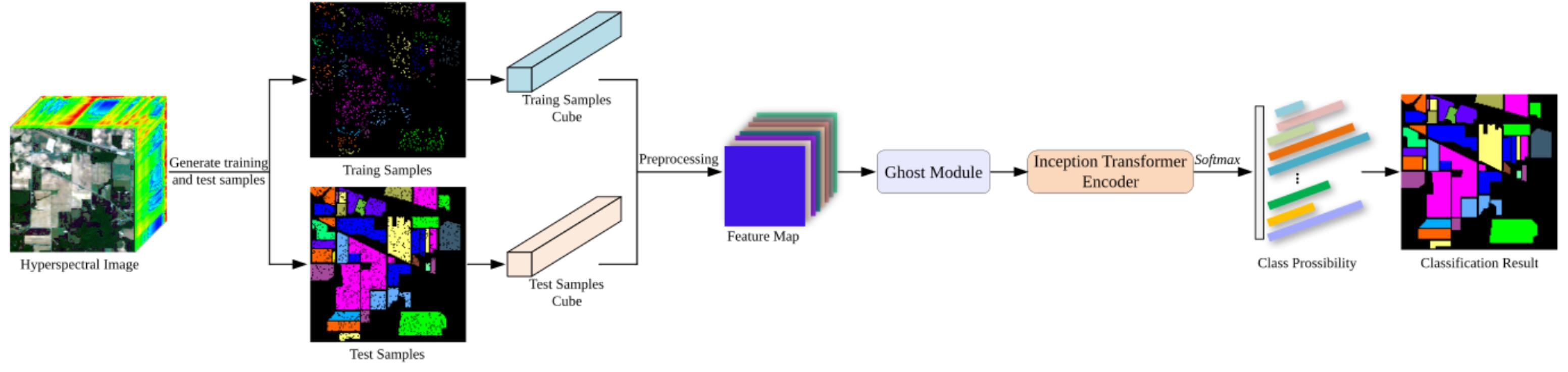
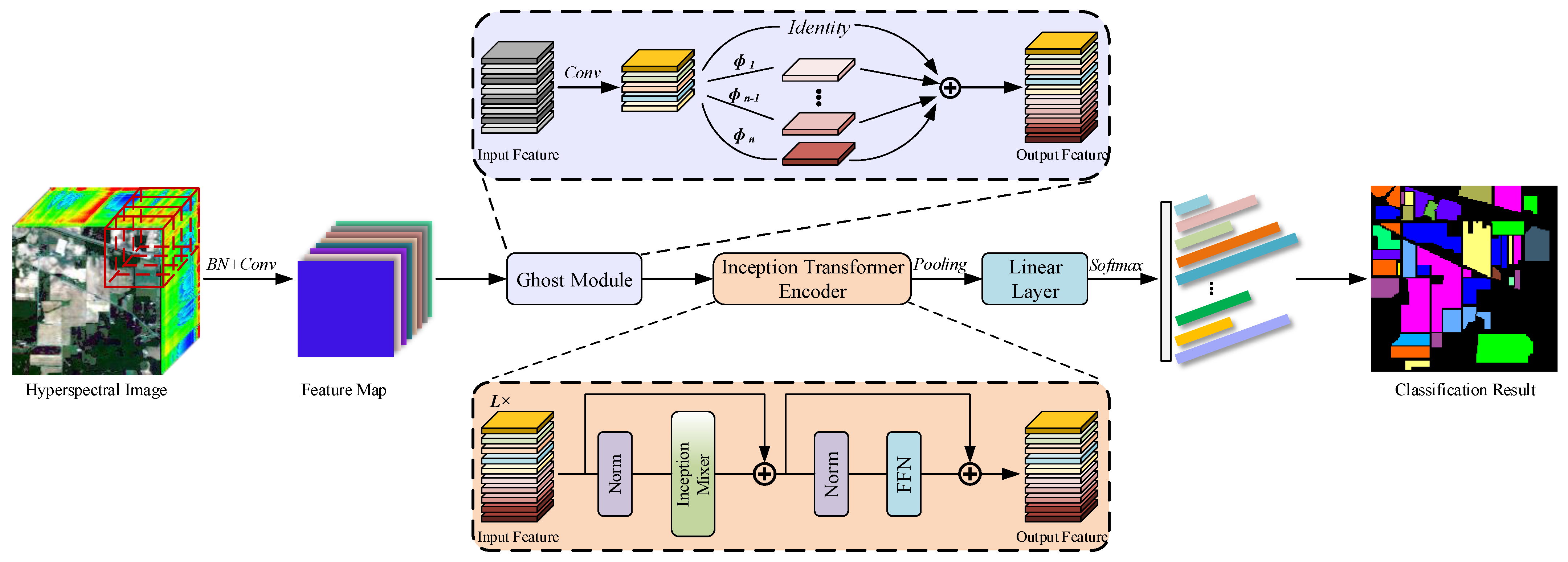
• Due to the corresponding reduction in critical information when extracting non-linear features for HSI, the Ghost Module is a novel cost-effective plug-and-play module, and is capable of generating more features with fewer parameters. It not only obtains more essential feature maps without changing the size of the output feature maps, but also significantly reduces the total number of parameters required, and the computational complexity.
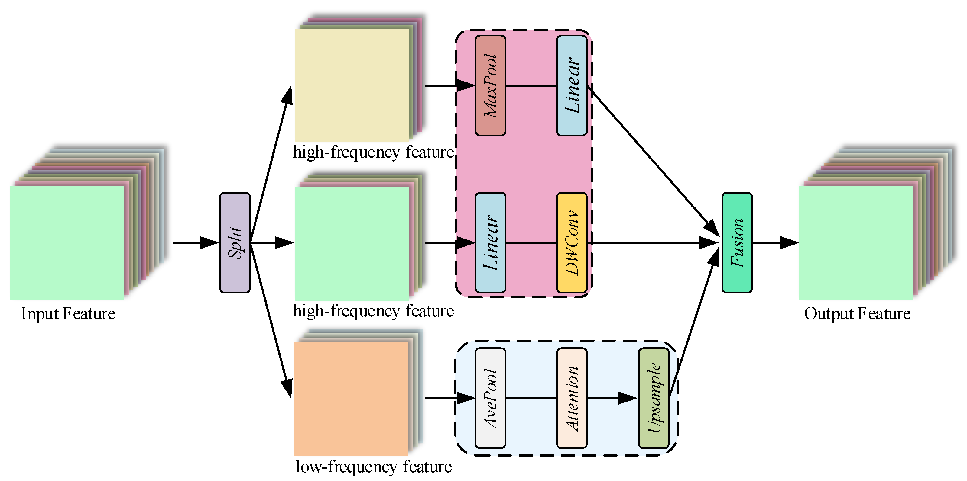
• Since the Ghost Module generates a large number of features, we introduce a simple but efficient Inception Transformer module to reasonably capture and exploit the global and local information of HSI. Inception mixer in the Inception Transformer uses the convolutional-maxpooling and self-attention paths run in parallel with the channel splitting mechanism to extract local details from high-frequency information, and global information from low-frequency information, respectively, thus reducing information loss.
• The proposed IFormer method is compared with other recent methods on four datasets, namely Indian Pines, University of Pavia, Salinas and LongKou, and the experimental results demonstrate that the model can achieve a high degree of accuracy and a low time complexity with a small number of samples.

The rest of the article is structured as follows. Section 2 introduces the relevant aspects of the proposed IFormer method. In Section 3, the sensitivity of the parameters of the method is analyzed mainly on four real HSI datasets, and the classification performance is compared with the classification results of other mainstream methods under different samples. Finally, Section 4 presents the conclusions and a discussion on future work.

2. Methods

In this section, we will focus on describing the structure and details of the IFormer, as shown in Figure 1 and Algorithm 1, by describing how to extract high- and low-frequency information from the HSI, so that the HSI features can be classified at a fine-grained level. The network structure consists of two main components: the Ghost Module processes the spectral features to generate more feature maps, and then the Inception Transformer can effectively learn from the feature maps to a combined feature containing both high- and low-frequency information from the ground. We elaborate on both parts in the following subsections.

Algorithm 1 IFormer method for HSI classification steps

Input:  The HSI dataset $\mathbf{X}\in {\mathbb{R}}^{h\times w\times b}$; 1D-CNN dimension $d=128$; spatial neighborhood block size s; channel ratio r; number of Inception Transformer layers L. 1: Construct a training patch and a test patch from the original HSI $\mathbf{X}$, with a training patch size of 20 and a test patch size to 300. 2: Patch $\mathbf{P}\in {\mathbb{R}}^{s\times s\times b}$ is processed into ${\mathbf{P}}^{\prime }\in {\mathbb{R}}^{s\times s\times d}$ using BN and 1D-CNN methods to extract spectral features and non-linear features. 3: Further, the feature map $\mathbf{Y}\in {\mathbb{R}}^{s\times s\times n}$ is generated by the Ghost Module in an inexpensive manner of operation. 4: forlto L do 5:    ${\mathbf{Z}}_l={\mathbf{Y}}_l+ITM\left(LN\left({\mathbf{Y}}_l\right)\right)$; 6:    ${\mathbf{H}}_l={\mathbf{Z}}_l+FFN\left(LN\left({\mathbf{Z}}_l\right)\right)$; 7: end for 8: $\mathbf{H}=\mathrm{Pooling}\left({\mathbf{H}}_L\right)$; 9: $\mathbf{F}=\mathrm{Softmax}\left(\mathbf{H}\right)$; Output:  Predicted labels for test pixel $\mathbf{F}$.

2.1. Ghost Module

Given the original HSI data $\mathbf{X}\in {\mathbb{R}}^{h\times w\times b}$, in which b is the number of the input channels, h is height of the input data, and w is the width of the input data. The spectral dimension of each pixel in $\mathbf{X}$ is b, forming a one-hot category vector $\mathbf{L}=({\mathit{l}}_1,{\mathit{l}}_2,···,{\mathit{l}}_{\mathit{C}})\in {\mathbb{R}}^{1\times 1\times \mathit{C}}$, where $\mathit{C}$ denotes the number of classes. Consider an HSI calculation for patch size as $\mathbf{P}\in {\mathbb{R}}^{s\times s\times b}$ using a BN and 1D-CNN model to obtain the spectral features ${\mathbf{P}}^{\prime }\in {\mathbb{R}}^{s\times s\times d}$, where s represents the spatial neighborhood block size and d indicates the dimension of the generated spectrum, and non-linear features were extracted. However, since the feature maps generated directly using CNN convolution have a large amount of redundancy, the Ghost Module was introduced to use a small amount of filtering in order to be able to generate more features to reduce the computational effort [48]. Feature maps that are outputted directly through the convolution layer commonly contain more redundancy, and there are some feature maps that have similarities. Therefore, it is not necessary to have a large number of parameters in order to generate these redundant feature maps. We assume that the output feature map is a “ghost” of the intrinsic feature map that can be transformed cheaply by a small number of parameters. Specifically, the Ghost Module is divided into two main stages.

In the first stage, we generate m intrinsic feature maps ${\mathbf{Q}}^{\prime }\in {\mathbb{R}}^{s\times s\times m}$ for the spectral feature ${\mathbf{P}}^{\prime }\in {\mathbb{R}}^{s\times s\times d}$ using a primary convolution layer, formulated as follows:

$${\mathbf{Q}}^{\prime }={\mathbf{P}}^{\prime }\otimes f+b$$

(1)

where ${\mathbf{Q}}^{\prime }\in {\mathbb{R}}^{s\times s\times m}$ is the output of the feature map, $m\le n$, ⊗ is the convolution operation, $f\in {\mathbb{R}}^{d\times k\times k\times m}$ are the convolution kernels in this stage, and b indicates offset. Furthermore, $k\times k$ represents the size of the convolution kernels f.

In the second stage, we perform a series of linear operations on each intrinsic feature in $\mathbf{Q}$’ in order to obtain the required n feature mappings, and therefore generate w “ghost” features in an inexpensive manner, according to the following function:

$${\mathbf{y}}_{ij}={\mathsf{\Phi }}_{i,j}\left({{\mathbf{q}}_i}^{\prime }\right)\forall i=1,...,m,j=1,...,w.$$

(2)

where ${{\mathbf{q}}_i}^{\prime }$ is the i-th feature map in ${\mathbf{Q}}^{\prime }$, and ${\mathsf{\Phi }}_{i,j}$ is the j-th (except the last one) linear arithmetic operation to generate the j-th “ghost” feature map ${\mathbf{y}}_{ij}$; ${{\mathbf{q}}_i}^{\prime }$ can generate one or more “ghost” feature maps ${\left\{{\mathbf{y}}_{ij}\right\}}_{j=1}^w$. ${\mathsf{\Phi }}_{i,w}$ is expressed as the identity mapping that maintains the intrinsic feature maps, as illustrated in the upper Ghost Module in Figure 1. With the calculation of Equation (2), $n=m·w$ feature maps $\mathbf{Y}=[{\mathbf{y}}_{11},···,{\mathbf{y}}_{mw}]$ can be obtained and used as the output data of Ghost Module, as displayed in the upper Figure 1. As can be seen from the computational complexity, the linear operation $\mathsf{\Phi }$ works on each channel, and its computational cost is much lower than that of ordinary convolution.

2.2. Inception Transformer

In order to effectively utilize the feature maps generated by Ghost Module, we further extract high- and low-frequency features from them using Inception Transformer. While the traditional Transformer performed well in building remote dependencies, it showed a lack of ability in capturing high-frequency local information, and the over-propagation of global information would enhance low-frequency representations and weaken high-frequency information parts, such as local information. In the case of HSI classification tasks, the high-frequency information is also discriminatory and can be beneficial for modeling scene details. Therefore, to compensate for the Transformer’s inability to capture high-frequency information, we introduce an efficient end-to-end form of the Inception Transformer structure [49], as depicted in the lower part of Figure 1.

Considering that CNNs obtain more local information through the sensory domain, an Inception token mixer (ITM) is proposed in the Inception Transformer, which transposes the powerful ability of CNNs to extract high-frequency representations into the Transformer, effectively combining the advantages of CNNs and Transformers, aiming to boost the extraction of high- and low-frequency information from the Transformer. The Inception Transformer differs from the previous Transformer in that instead of directly feeding a series of patch tokens into MSAs, the input features are first segmented proportionally along the channel dimension, and then for the segmented features, they are fed into a high-frequency mixer and a low-frequency mixer, respectively. The high-frequency mixer contains two operations: maximum pooling operation and parallel convolution, while the low-frequency mixer is mainly performed using self-attention. Technically, the input feature maps are given as $\mathbf{Y}\in {\mathbb{R}}^{s\times s\times n}$, and $\mathbf{Y}$ is decomposed into high-frequency feature maps ${\mathbf{Y}}_{\mathbf{h}}\in {\mathbb{R}}^{s\times s\times n_h}$ and low-frequency feature maps ${\mathbf{Y}}_{\mathbf{l}}\in {\mathbb{R}}^{s\times s\times n_l}$ along the channel dimension, $n=n_h+n_l$, where $n_h=n\ast \mathbf{r}$, and r denotes the channel ratio. ${\mathbf{Y}}_{\mathbf{h}}$ and ${\mathbf{Y}}_{\mathbf{l}}$ are then assigned to the high-frequency mixers and low-frequency mixers, respectively.

High-frequency mixer: Since the maximum filter is sensitive to features and the convolution operation is equally detail-aware, we use a parallel structure for detailed features to learn the high-frequency components, (i.e., local features and boundaries). We divided the high-frequency component ${\mathbf{Y}}_{\mathbf{h}}$, in the channel dimension into ${\mathbf{Y}}_{\mathbf{h}\mathbf{1}}\in {\mathbb{R}}^{s\times s\times \frac{n_h}{\mathbf{2}}}$ and ${\mathbf{Y}}_{\mathbf{h}\mathbf{2}}\in {\mathbb{R}}^{s\times s\times \frac{n_l}{\mathbf{2}}}$. For the high-frequency mixer, ${\mathbf{Y}}_{\mathbf{h}\mathbf{1}}$ is fed into a max-pooling and a linear layer, and ${\mathbf{Y}}_{\mathbf{h}\mathbf{2}}$ is embedded in a linear layer and a deep convolution layer, as presented in Figure 2.

Both of the output feature maps can be expressed using the following formulas:

$${\mathbf{Z}}_{\mathbf{h}\mathbf{1}}=FC\left(MaxPool\left({\mathbf{Y}}_{\mathbf{h}\mathbf{1}}\right)\right)$$

(3)

$${\mathbf{Z}}_{\mathbf{h}\mathbf{2}}=DWConv\left(FC\left({\mathbf{Y}}_{\mathbf{h}\mathbf{2}}\right)\right)$$

(4)

where ${\mathbf{Z}}_{\mathbf{h}\mathbf{1}}$ and ${\mathbf{Z}}_{\mathbf{h}\mathbf{2}}$ are the output feature maps of the high-frequency mixers.

Low-frequency mixer: We still use MSA to pass information between all tokens of the low-frequency mixer, due to its excellent ability to extract low-frequency information. Although the self-attention mechanism is highly capable of targeting global representations, it can be computationally intensive at a shallow level for large resolution feature maps. Thus, to reduce the spatial scale of ${\mathbf{Y}}_{\mathbf{l}}$, only the original spatial dimension is recovered through the use of an average pooling layer before the self-attention operation, and an upsampling layer after the self-attention operation. Such operations can effectively reduce the consumption of computational costs and enable attention operations to be centrally embedded in the global information. The output feature maps can be expressed using the following formula:

$${\mathbf{Z}}_{\mathbf{l}}=Upsample\left(MSA\left(AvePool\left({\mathbf{Y}}_{\mathbf{l}}\right)\right)\right)$$

(5)

where ${\mathbf{Z}}_{\mathbf{l}}$ means the output feature maps of low-frequency mixers.

Fusion: In the end, we concatenate the channel dimension of the high-frequency mixers and the low-frequency mixer:

$${\mathbf{Z}}_c=Concat({\mathbf{Z}}_{\mathbf{l}},{\mathbf{Z}}_{\mathbf{h}\mathbf{1}},{\mathbf{Z}}_{\mathbf{h}\mathbf{2}})$$

(6)

Considering that the upsampling operation in Equation (5) would in turn select the value of the closest point at each location without considering the other points; this would lead to excessive smoothing between neighboring markers. Therefore, a fusion module is proposed that subtly compensates this problem by exchanging information between patches in a deep convolution while maintaining a linear layer across channels, so that, like the previous Transformer, it can continue working at each position. The final output features are described below:

$$\mathbf{Z}=FC({\mathbf{Z}}_c+DWConv\left({\mathbf{Z}}_c\right))$$

(7)

Inception Transformer has a feed-forward network (FFN), as does ViT, but with the difference being that Inception Transformer replaces the MSA mechanism with the ITM and applies LayerNorm (LN) before ITM and FFN. Therefore, Inception Transformer can eventually be expressed using the following formulae:

$$\mathbf{Z}=\mathbf{Y}+ITM\left(LN\right(\mathbf{Y}\left)\right)$$

(8)

$$\mathbf{H}=\mathbf{Z}+FFN\left(LN\right(\mathbf{Z}\left)\right)$$

(9)

With the Inception Transformer module, the input feature size is equal to the output feature size. The output feature patch is passed through a linear layer and a $\mathit{softmax}$ function to calculate the probability that the output feature belongs to one of the feature categories for the final classification, and the label with the highest probability value is the category in which the sample is located.

3. Experimental Result and Analysis

In order to verify the effectiveness of the proposed IFormer model in HSI classification, we experiment and analyze it in this section. First, the dataset used for the experiments is briefly described and compared with other advanced algorithms on the dataset, as well as parameter analysis. Finally, to authenticate the validity and competitiveness of the proposed method, we perform IFormer and ablation experiments in terms of time cost and under different samples.

All classification experiments were performed on a workstation equipped with Intel Core i9-10900KF, Nvidia Geforce GTX3070Ti GPU, and 32 GB RAM. The IFormer model proposed in this paper is implemented using the Python language with PyTorch library, and other comparison methods use the corresponding original experimental environment.

3.1. DataSets Description

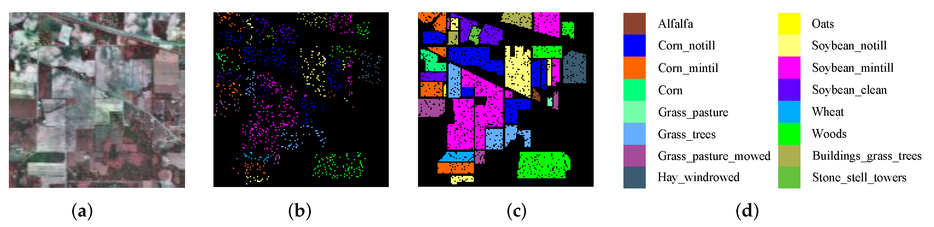
3.1.1. Indian Pines (IP) Dataset

The Indian Pines dataset was collected using an Airborne Visible/Infrared Imaging Spectrometer (AVIRIS) sensor in Northwestern Indiana, USA. The 24 absorbing bands are removed, so that the next 200 bands are retained out of 224 spectral bands. The dataset has a spatial size of 145 × 145 pixels, a spatial resolution of 20 m/pixel, a spectral resolution of 400–2500 nm, and a labeled pixels count of 10,249, covering 16 object categories. The composite images, training set, test set, and legend are presented in Figure 3, and the number of training samples, the number of validation sets, and the number of test sets for the corresponding categories are provided in

Table 1. The number of training sets and test samples covered by each surface selected on the IP dataset, and the number of all in each class.

Class No.	Class Name	Total Sample	Training	Validation	Test
1	Alfalfa	46	5	2	39
2	Corn_N	1428	143	14	1271
3	Corn_M	830	83	8	739
4	Corn	237	24	2	211
5	Grass_P	483	49	4	430
6	Grass_T	730	73	7	650
7	Grass_P_M	28	3	2	23
8	Hay_W	478	48	4	426
9	Oats	20	2	1	17
10	Soybean_N	972	98	9	865
11	Soybean_M	2455	246	24	2185
12	Soybean_C	593	60	6	527
13	Wheat	205	21	2	182
14	Woods	1265	127	12	1126
15	Buildings_G_T	386	39	3	344
16	Stone_S_T	93	10	2	81

.

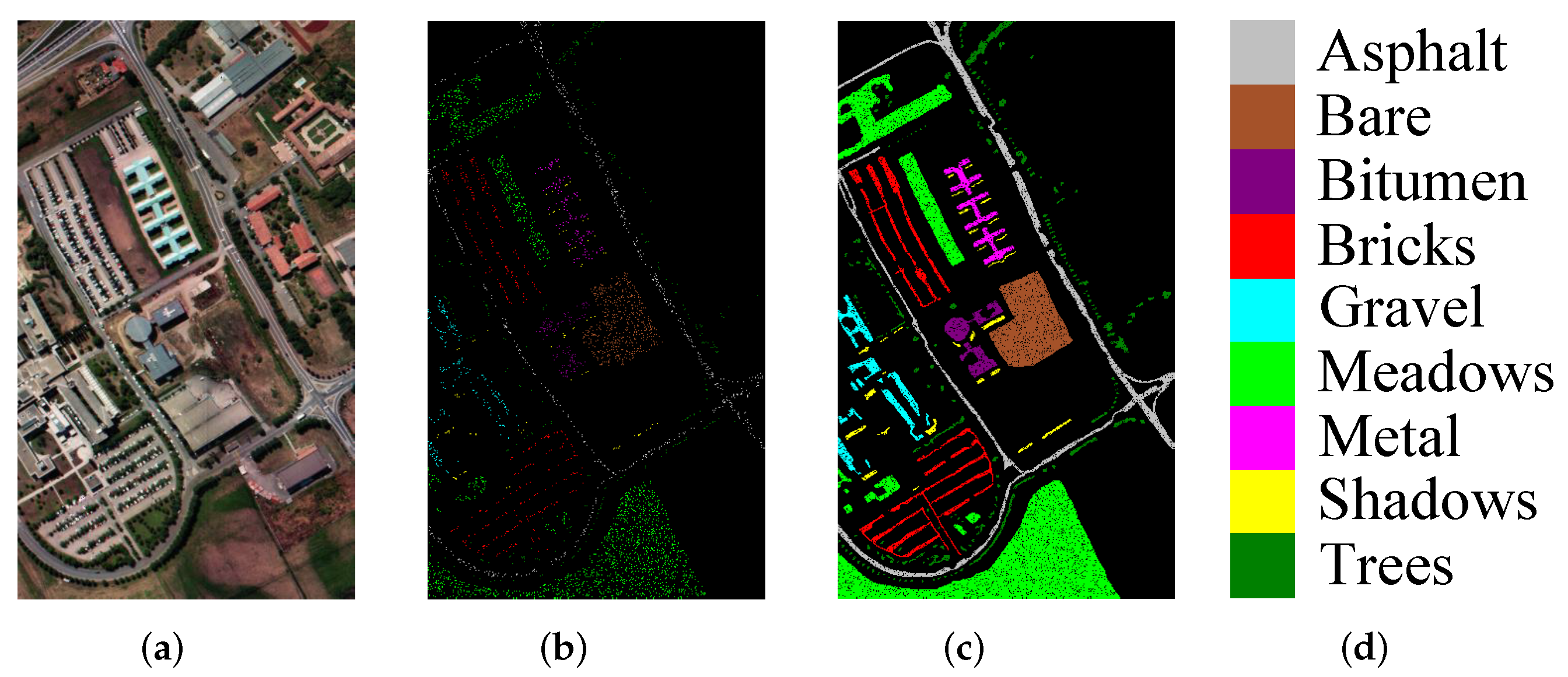
3.1.2. University of Pavia (UP) Dataset

The University of Pavia dataset was collected by the ROSIS-03 sensor at University of Pavia, Italy, in 2002, measuring 610 × 340 pixels with a spatial resolution of approximately 1.3 m. The dataset contains nine main landcover classes in the wavelengths range of 0.43∽0.86 $\mathsf{\mu }$m, with a total of 42,776 labeled pixels, in addition to the background. The original dataset had 115 bands, and after removing 12 high-noise bands, the remaining 103 bands were selected for the experiment. Figure 4 and

Table 2. The number of training sets and test samples covered by each surface selected on the UP dataset, and the number of all in each class.

Class No.	Class Name	Total Sample	Training	Validation	Test
1	Asphalt	6631	67	66	6498
2	Meadows	18,649	187	187	18,275
3	Gravel	2099	21	21	2057
4	Trees	3064	31	31	3002
5	Metal	1345	14	14	1317
6	Bare	5029	51	50	4928
7	Bitumen	1330	14	11	1305
8	Bricks	3682	37	37	3608
9	Shadows	947	10	10	927

give detailed information on the UP dataset.

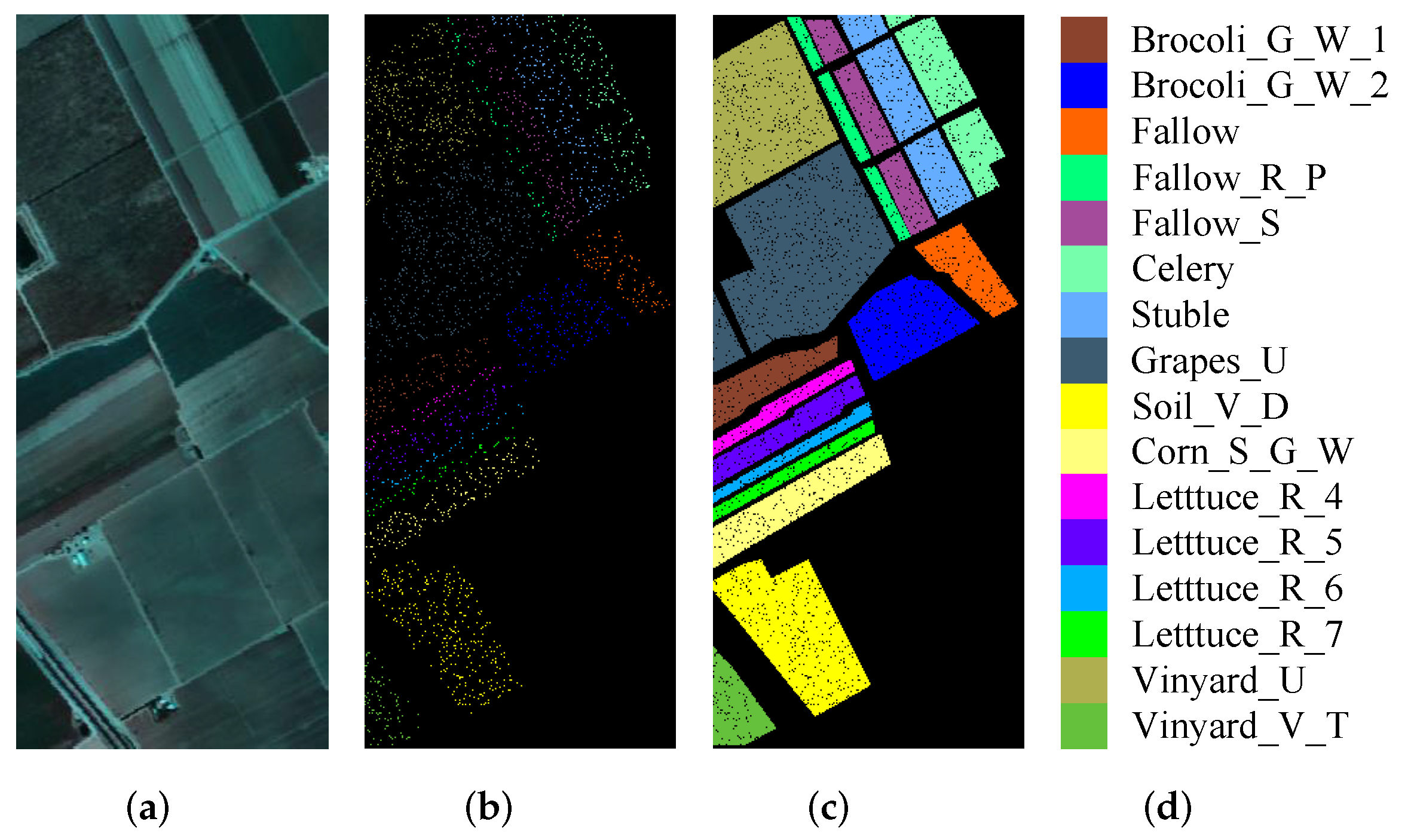
3.1.3. Salinas Valley (SV) Dataset

The dataset scene has a spatial resolution of 3.7 m/pixel and was acquired using AVIRIS sensor photography in Salinas Valley, California. Additionally, the scene consists of 512 × 217 pixels, and after removing 20 water vapor bands, 204 water vapor bands remain. The SV dataset contains 16 classes and 54,149 pixels as ground truth. Figure 5 shows the composition map, training label map, test label map, ground truth, and legend of the SV dataset. The training set, validation set, and test set are picked according to the description in

Table 3. The number of training sets and test samples covered by each surface selected on the SV dataset, and the number of all in each class.

Class No.	Class Name	Total Sample	Training	Validation	Test
1	Brocoli_G_W_1	2009	21	20	1968
2	Brocoli_G_W_2	3726	38	36	3652
3	Fallow	1976	20	20	1936
4	Fallow_R_P	1394	14	14	1366
5	Fallow_S	2678	27	26	2625
6	Celery	3579	36	36	3507
7	Stubble	3959	40	40	3879
8	Grapes_U	11,271	113	113	11,045
9	Soil_V_D	6203	63	62	6078
10	Corn_S_G_W	3278	33	33	3212
11	Letttuce_R_4	1068	11	11	1046
12	Letttuce_R_5	1927	20	19	1888
13	Letttuce_R_6	916	10	9	897
14	Letttuce_R_7	1070	11	11	1048
15	Vinyard_U	7268	73	73	7122
16	Vinyard_V_T	1807	19	18	1770

.

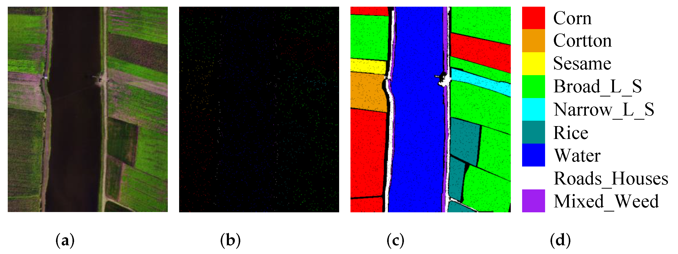
3.1.4. WHU-Hi-LongKou (LK) Dataset

The WHU-Hi-LongKou dataset was photographed using an 8 mm focal length hyperspectral imager in the LongKou town area of Hubei Province, China [50,51]. The spatial resolution of the airborne hyperspectral images is approximately 0.463 m. The dataset is 550 × 400 pixels in size and has 270 bands, located between 400∼1000 nm. The research scenario focuses on crop areas, with nine landcover types such as corn, cotton, and sesame. The main falsecolor image of the LK dataset, the training sample set, the test set, and the reference color code are shown in Figure 6. For the experiment, 1% of datasets was used for each of training and validation, and 98% was used as the test set, as shown in

Table 4. The number of training sets and test samples covered by each surface selected on the LK dataset, and the number of all in each class.

Class No.	Class Name	Total Sample	Training	Validation	Test
1	Corn	34,511	346	346	33,819
2	Cotton	8374	84	84	8206
3	Sesame	3031	31	30	2970
4	Broad_L_S	63,212	633	632	61,947
5	Narrow_L_S	4151	42	41	4068
6	Rice	11,854	119	118	11,617
7	Water	67,056	671	670	65,715
8	Roads_Houses	7124	72	71	6981
9	Mixed_Weed	5229	53	52	5124

.

3.2. Experimental Setting and Analysis

3.2.1. Experimental Setting

The overall accuracy (OA), average accuracy (AA), and kappa coefficient (Kappa) are employed to evaluate the superiority and effectiveness of the algorithm. OA means the probability of correctly predicted labels among all labels, AA is expressed as the number of correctly predicted labels in each category as a percentage of the number of all samples in that category, and the kappa coefficient is used to define the identity between the tested true labels and the predicted labels.

In addition, to maintain the fairness of the experiment, all comparison methods, as well as the proposed method, were executed 10 times with randomly selected training samples, as well as the obtained means of OA, AA, and Kappa, and the standard deviations, with the middle number of () denoted as the standard deviation of the three evaluation metrics. For the training process of the model on the four datasets, we use cross-entropy as the loss function, and the optimizer updates the parameters of the model by stochastic gradient descent (SGD) to avoid overfitting, with the learning rate and epoch set to 0.001 and 150, respectively.

• SVM [52] is mainly used as a traditional classification method to extract the spectral information of HSI using LibSVM toolbox [53], with radial basis function (RBF) kernel, and to perform five-fold cross-validation.
• The overall structure of SSRN [35] is a combination of 3D-CNN [54] and ResNet [30], where the input size is 7 × 7 × B, and B denotes the number of bands.
• The 1D-CNN [31] is structured using a convolutional layer with a filter size of 20, a BN layer, a pooling layer of size 5, a ReLU activation layer, and finally, a $softmax$ function that can extract only the spectral feature of HSI.
• The 2D-CNN [55] is a network containing two 2D-CNN layers, three ReLU activation layers, and a max-pooling layer, which has an input patch size of 7 × 7 × B.
• FDSSC [36] is proposed on the basis of DenseNet, [56] combined with the spectral and spatial structure of HSI. The input patch size is 9 × 9 × B, which we reduce to 5 × 5 × B because the LK dataset is too large and the computational memory is insufficient.
• The structure of DBDA [38] is composed of DenseNet as the backbone network and the DANet [57] attention mechanism, with an input patch size of 9 × 9 × B and the same size of 5 × 5 × B on the LK dataset.
• CGCNN [34] takes the entire HSI as the input and extracts HSI features by guiding the CNN convolution kernel through features, where the convolution kernel size is 5 × 5.
• SF [45]: SF as a Transformer structure, learns local spectral features from HSI adjacent bands and skips connections using cross-layers; the input patch size is 7 × 7 × 3. Since the LK dataset scene is too large, the input size is set to 5 × 5 × 3.

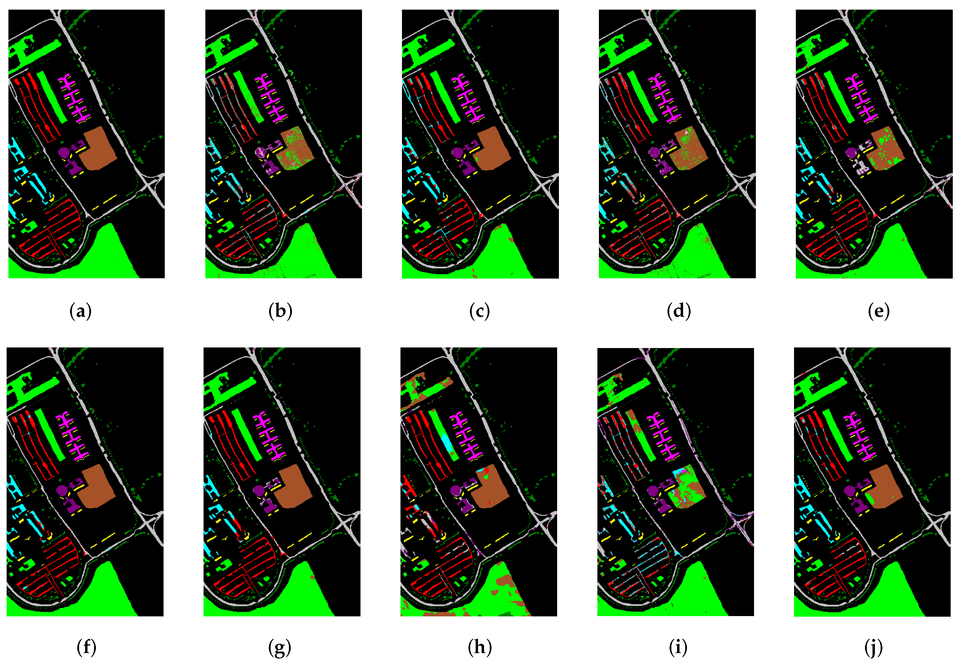
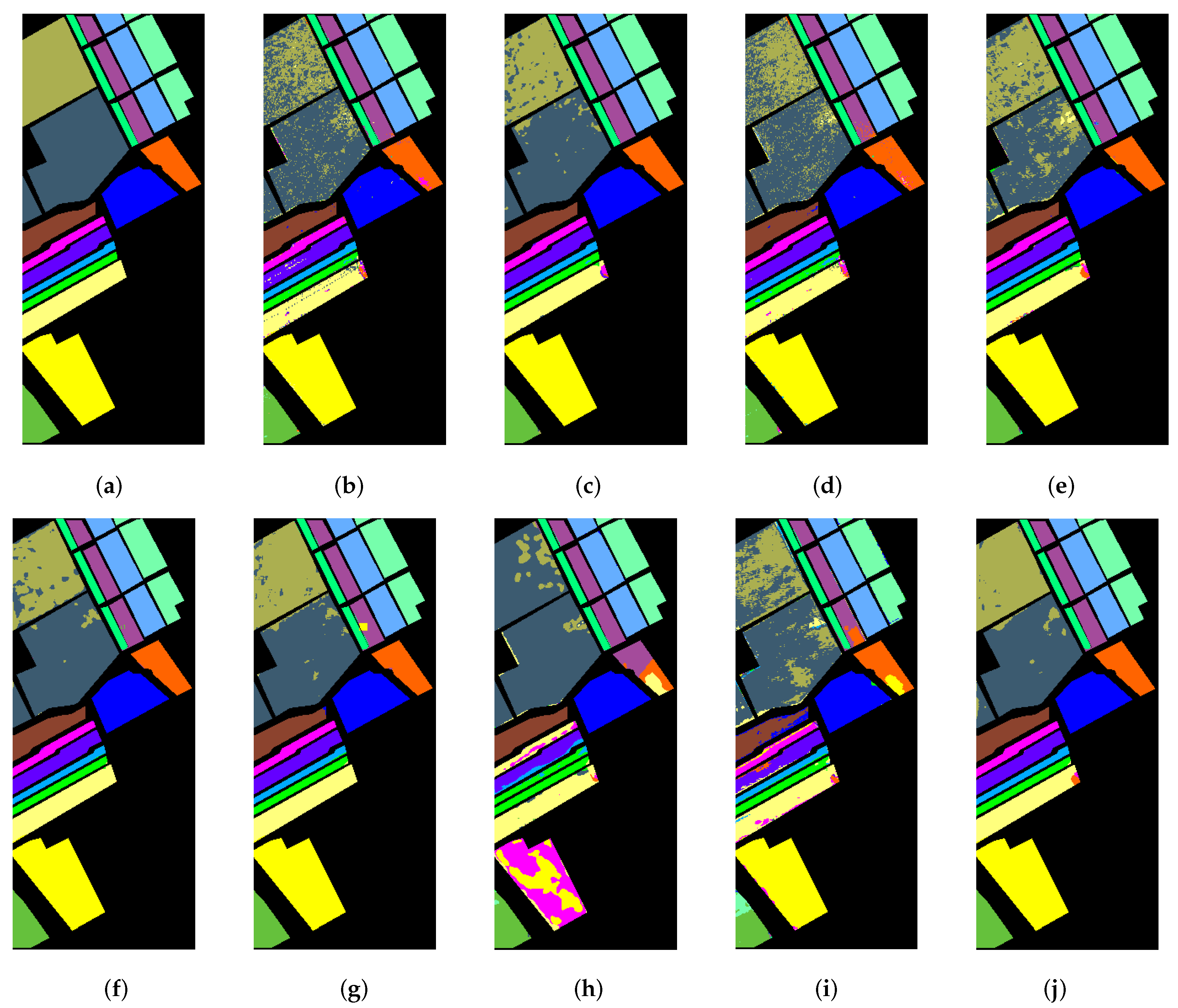
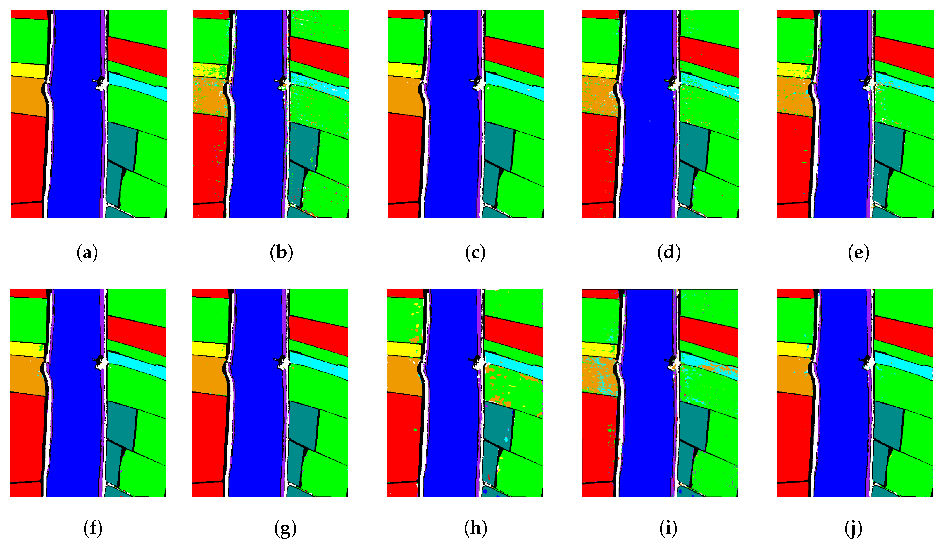
3.2.2. The Proposed Algorithm Compared with the Advancement of Existing Methods

First, the performance of the proposed method, IFormer, is compared with other advanced algorithms on IP datasets with small sample scenarios. A proportion of 10% of the samples are selected as training samples, and 1% and 89% of the samples are used as the validation and test sets, respectively. From the qualitative analysis in

Table 5. Accuracy comparison of different methods on IP dataset.

Class No.	Classification Accuracy Obtained by the Proposed Method and Different Comparison Methods (in %) 1
	SVM	SSRN	1D-CNN	2D-CNN	FDSSC	DBDA	CGCNN	SF	IFormer
1	65.61(15.6)	97.85(6.42)	33.41(7.32)	70.48(17.4)	99.72(0.81)	95.37(7.67)	94.51(6.54)	25.12(6.45)	80.98(19.7)
2	79.69(1.98)	97.14(2.27)	79.30(2.18)	93.19(1.67)	98.45(1.54)	98.18(1.06)	98.04(1.08)	87.85(4.05)	97.95(0.54)
3	69.73(2.68)	98.01(1.34)	64.32(3.41)	92.51(2.20)	98.47(2.12)	98.81(1.08)	90.19(6.60)	86.15(2.14)	99.31(0.27)
4	62.44(8.34)	96.71(3.74)	52.39(6.97)	86.19(4.18)	98.03(2.83)	97.04(4.03)	92.79(3.66)	90.98(4.49)	96.16(3.17)
5	89.40(2.74)	98.63(1.04)	88.34(4.91)	95.47(2.43)	99.23(1.09)	97.41(1.72)	96.36(2.98)	89.07(1.71)	97.49(1.54)
6	95.48(1.85)	99.04(0.97)	97.51(0.71)	99.16(0.36)	98.84(0.97)	99.25(1.05)	99.43(0.82)	97.64(1.68)	98.95(0.29)
7	76.40(7.41)	50.00(50.0)	36.40(24.5)	74.80(12.9)	94.44(12.9)	92.67(13.5)	98.80(1.83)	48.40(8.48)	85.80(15.3)
8	98.09(1.36)	98.63(1.41)	97.65(2.18)	99.76(0.20)	99.31(1.36)	100.00(0.0)	99.92(0.15)	99.62(0.31)	100.00(0.0)
9	42.78(19.8)	10.00(30.0)	28.33(20.3)	90.55(7.47)	79.56(28.6)	95.06(7.59)	99.44(1.66)	38.23(17.6)	65.88(20.5)
10	78.40(3.14)	92.30(9.24)	71.70(4.72)	94.36(2.17)	95.70(4.06)	95.73(3.18)	95.09(2.42)	89.92(2.35)	98.19(2.41)
11	85.54(0.89)	97.51(4.13)	80.65(1.99)	94.99(0.95)	98.31(1.42)	99.07(0.60)	98.47(1.28)	93.42(3.03)	98.98(0.62)
12	73.60(3.56)	95.58(3.06)	77.75(2.45)	83.29(4.37)	91.32(18.5)	98.16(0.60)	96.10(2.83)	81.53(4.48)	96.33(2.41)
13	96.41(2.64)	99.56(0.72)	98.43(1.14)	99.94(0.16)	99.24(1.55)	98.77(2.17)	99.56(0.21)	99.78(0.26)	99.78(0.27)
14	94.92(2.37)	99.27(0.37)	95.01(1.04)	98.10(1.04)	98.79(0.96)	98.84(0.84)	99.35(0.52)	95.56(1.05)	99.59(0.27)
15	57.12(3.74)	98.05(1.75)	63.48(6.36)	89.91(4.69)	98.25(2.40)	98.62(1.33)	98.82(1.09)	60.83(6.22)	98.34(0.80)
16	85.18(4.02)	96.21(5.32)	84.16(3.06)	96.78(4.39)	96.41(4.30)	93.39(6.67)	98.19(3.37)	99.03(1.18)	99.88(0.37)
OA(%)	83.12(0.90)	97.11(1.55)	80.91(0.75)	94.28(0.38)	97.19(2.95)	98.28(0.61)	97.31(0.75)	90.05(0.89)	98.44(0.45)
AA(%)	80.69(1.03)	89.03(3.45)	71.80(2.65)	91.22(1.12)	96.50(2.39)	97.27(1.29)	97.19(0.82)	80.20(1.71)	94.54(3.13)
Kappa	78.17(2.14)	96.71(1.77)	78.16(0.85)	93.47(0.44)	96.82(3.30)	98.04(0.69)	96.93(0.85)	88.64(1.00)	98.22(0.52)

¹ Optimal precision is bold.

, it is more intuitive that the proposed method, IFormer, shows some advantages in both the OA and Kappa evaluation metrics. IFormer yields 15.3% accuracy relative to SVM, which indicates that deep learning shows a clear advantage in HSI classification. In addition, among the deep learning methods, IFormer has some advantages over other recent advanced algorithms, such as CGCNN and DBDA, in terms of recognition accuracy in categories such as Corn_M, Hay_W, and Soybean_N, as seen in Figure 7. Nevertheless, the classification accuracy of IFormer for Alfalfa is 18.7% lower than that of FDSSC, and 33.56% lower than that of CGCNN for oats, which may be due to the imbalance in the number of samples in the dataset scenario; especially as the category of Oats contains only 20 samples, and as we selected the training samples proportionally, it is thus easy to cause IFormer to pay less attention to the category with fewer sample categories to focus less attention. In addition, the proposed method is almost 10% higher than the SF in the OA and Kappa evaluation metrics, which indicates that IFormer makes full use of the high- and low-frequency information in HSI.

Table 6. Accuracy comparison of different methods on UP dataset.

Class No.	Classification Accuracy Obtained by the Proposed Method and Different Comparison Methods (in %)
	SVM	SSRN	1D-CNN	2D-CNN	FDSSC	DBDA	CGCNN	SF	IFormer
1	89.56(3.10)	97.82(2.41)	91.07(1.52)	94.09(1.74)	97.00(1.89)	97.21(1.96)	92.41(2.28)	72.80(7.11)	99.94(0.06)
2	88.36(3.04)	95.26(5.24)	81.74(2.41)	90.02(3.85)	99.46(0.29)	98.15(2.07)	95.23(2.71)	89.33(4.91)	99.85(0.04)
3	75.27(6.85)	97.75(3.60)	75.70(4.33)	83.96(4.29)	85.84(15.7)	96.94(4.22)	97.29(5.33)	57.48(8.14)	94.18(1.60)
4	77.20(4.41)	90.00(3.67)	84.18(1.83)	90.00(1.87)	98.60(0.88)	88.97(4.78)	91.98(8.47)	94.15(3.29)	97.13(0.26)
5	94.04(1.93)	99.60(0.51)	87.71(1.39)	90.57(1.81)	99.45(0.31)	96.63(1.45)	98.51(0.78)	99.91(0.10)	99.97(0.05)
6	68.03(4.39)	85.20(16.7)	69.76(3.23)	78.21(3.72)	99.45(0.31)	97.46(3.33)	39.97(21.9)	33.61(9.55)	97.09(2.13)
7	91.92(0.74)	99.18(0.46)	96.34(0.45)	98.44(0.36)	98.96(0.31)	99.41(0.40)	86.13(9.54)	95.12(1.74)	100.00(0.0)
8	98.33(1.55)	99.91(0.09)	98.61(0.64)	99.74(0.37)	92.69(5.68)	99.37(1.13)	99.99(0.02)	67.67(10.2)	92.06(3.03)
9	99.97(0.05)	99.30(1.43)	99.55(0.26)	96.99(2.96)	98.45(1.63)	93.89(4.84)	99.86(0.21)	96.97(2.02)	95.64(1.03)
OA(%)	88.68(0.68)	96.62(1.79)	90.34(0.42)	94.05(0.68)	97.27(1.12)	97.49(0.56)	88.38(4.60)	77.73(1.66)	98.30(0.46)
AA(%)	86.96(1.23)	96.00(2.06)	87.19(0.59)	91.34(0.63)	96.65(1.30)	96.95(0.65)	89.04(3.09)	78.56(1.38)	97.32(0.53)
Kappa	84.84(0.92)	95.54(2.35)	87.12(0.57)	92.08(0.91)	96.38(1.30)	96.67(0.75)	85.08(5.66)	70.29(2.05)	97.74(0.61)

displays the classification results that were given using the comparison method on the UP dataset, and Figure 8 presents a classification map for the corresponding algorithm. As we can visually observe in Table 6, IFormer performs 2% more accurately than most classification methods for the four categories of Asphalt, Meadows, Bitumen, and Metal, and with 100% accuracy for Bitumen. DBDA introduces the DANet attention mechanism [56], and expects to be able to learn detailed information from HSI, but the accuracy in classifying the Trees categories is not as good as it should be. All three classification metrics of DBDA with the introduction of the DANet attention mechanism outperformed FDSSC and CECNN, because the attention mechanism allows for more attention to important detailed information in the HSI. The proposed method then achieves the best classification results and performance compared with the method that also introduces the attention mechanism; one of the reasons for this is that the Ghost Module in IFormer is able to generate more important features, while the Inception Transformer considers high- and low-frequency information in the feature map, thus highlighting the respective represented features.

We further compare the classification results of IFormer with other advanced algorithms in the SV scene; therefore, 1% of the training samples are randomly selected in this scene, and it can be seen in

Table 7. Accuracy comparison of different methods on SV dataset.

Class No.	Classification Accuracy Obtained by the Proposed Method and Different Comparison Methods (in %)
	SVM	SSRN	1D-CNN	2D-CNN	FDSSC	DBDA	CGCNN	SF	IFormer
1	99.73(0.57)	99.98(0.02)	99.47(0.48)	99.25(0.67)	100.00(0.0)	100.00(0.0)	100.00(0.0)	87.72(10.6)	100.00(0.0)
2	99.09(0.28)	99.80(0.25)	99.59(1.05)	99.32(1.40)	99.93(0.13)	99.97(0.04)	99.81(0.35)	99.09(0.79)	100.00(0.0)
3	92.50(1.65)	98.16(1.33)	98.17(1.11)	97.10(2.71)	98.61(1.64)	98.80(1.20)	33.29(6.20)	92.51(5.26)	100.00(0.0)
4	97.20(0.63)	98.90(0.58)	98.89(0.29)	99.23(0.31)	97.81(2.27)	95.72(3.65)	99.83(0.09)	96.31(1.42)	98.60(0.39)
5	97.19(1.04)	99.84(0.24)	97.99(0.57)	97.20(1.11)	99.51(0.60)	97.14(4.92)	76.48(22.1)	89.19(5.51)	99.57(0.25)
6	98.69(0.82)	100.0(0.00)	99.65(0.12)	99.56(0.25)	99.99(0.01)	99.65(0.61)	99.91(0.05)	99.99(0.12)	100.00(0.0)
7	99.95(0.06)	99.98(0.03)	99.61(0.19)	99.84(0.23)	100.00(0.0)	99.99(0.01)	99.85(0.12)	96.09(2.62)	99.96(0.04)
8	75.58(1.05)	91.72(3.98)	86.04(1.17)	84.13(1.48)	95.33(4.39)	93.27(6.55)	88.08(7.10)	83.84(6.82)	95.79(0.91)
9	98.73(0.35)	99.69(0.13)	99.46(0.31)	99.68(0.34)	99.60(0.29)	99.36(0.58)	84.50(17.4)	98.75(0.39)	100.00(0.0)
10	88.95(2.66)	99.11(0.73)	92.51(1.38)	91.87(2.29)	98.34(1.41)	98.63(1.19)	86.50(6.46)	92.76(2.64)	96.50(0.59)
11	90.58(4.15)	97.56(2.39)	95.73(2.66)	95.85(1.84)	96.99(2.29)	96.57(3.05)	89.53(22.1)	89.83(5.80)	99.66(0.54)
12	96.24(0.79)	99.31(0.83)	99.92(0.11)	99.77(0.42)	99.19(0.79)	99.32(1.37)	85.14(14.5)	91.70(9.17)	99.60(0.58)
13	93.37(3.23)	99.25(1.04)	98.88(0.84)	97.87(1.69)	99.57(0.68)	99.83(0.15)	34.97(31.5)	96.25(3.79)	99.97(0.07)
14	94.75(2.30)	98.68(0.88)	90.82(3.83)	95.89(1.48)	98.57(1.01)	96.97(3.07)	98.34(1.77)	97.70(2.27)	99.39(0.35)
15	74.66(2.89)	89.14(5.35)	65.08(2.66)	74.65(3.31)	84.68(12.9)	89.05(11.5)	60.47(25.6)	64.95(13.8)	97.37(0.78)
16	98.08(0.71)	100.0(0.00)	96.76(2.11)	93.58(4.83)	99.46(0.83)	99.97(0.08)	97.21(1.59)	82.17(5.75)	99.77(0.17)
OA(%)	89.64(0.48)	96.31(0.36)	91.20(0.50)	91.96(0.56)	95.73(2.25)	95.84(2.40)	84.02(4.30)	88.47(2.39)	98.46(0.17)
AA(%)	93.46(0.51)	98.19(0.19)	94.91(0.52)	95.30(0.49)	97.97(0.74)	97.77(0.98)	83.37(4.37)	91.18(2.56)	99.14(0.10)
Kappa	88.24(0.53)	95.90(0.40)	90.19(0.56)	91.05(0.62)	95.26(2.48)	95.37(2.66)	82.17(4.81)	87.14(2.68)	98.28(0.19)

that the classification accuracy of all deep learning methods reaches more than 90%, except for two methods, CECNN and SF. In addition, as seen in Table 7, SVM, 1D-CNN, and 2D-CNN all focus on only one type of feature in terms of the spectral and spatial features, and to some extent, they do not effectively combine the spectral and spatial features or utilize additional information, resulting in information loss. Although both the SSRN and FDSSC methods utilize spatial-spectral binding techniques and are not obvious between the classification results, both methods are computationally expensive and have complex network structures. In contrast, SF and IFormer both have simple structures, but the classification accuracy of SF is lower than that of both traditional SVM methods, especially as the classification accuracy for Bare is only 33.61%. However, IFormer achieves the highest OA result of 98.46%, with 99.39% and 97.37% classification accuracies for the categories Lettuce_R_7 and Vinyard_U, respectively, which reflects the excellent ability of the IFormer method to extract local detail information. Finally, as can be observed in Figure 9, IFormer is able to extract information from global and local regions in the HSI better, with less misclassification.

As the LK dataset was taken using an unmanned aerial vehicle (UAV), and therefore has better spatial resolution and less noise interference, comparing the results of the previous three datasets, each method has higher results on the LK dataset, and

Table 8. Accuracy comparison of different methods on LK dataset.

Class No.	Classification Accuracy Obtained Using the Proposed Method and Different Comparison Methods (in %)
	SVM	SSRN	1D-CNN	2D-CNN	FDSSC	DBDA	CGCNN	SF	IFormer
1	98.91(0.27)	99.84(0.09)	99.11(0.34)	98.94(0.33)	99.43(0.12)	99.83(0.07)	98.90(0.73)	99.06(0.89)	99.97(0.01)
2	86.00(2.70)	98.35(2.42)	86.89(3.35)	87.72(1.97)	98.94(1.17)	98.28(2.61)	95.60(5.03)	84.99(2.51)	99.62(0.20)
3	76.79(2.82)	99.38(1.08)	81.71(4.10)	82.32(5.09)	99.60(0.33)	97.02(5.36)	93.25(5.09)	80.32(8.96)	98.70(0.58)
4	97.22(0.24)	99.26(0.55)	97.26(0.48)	97.01(0.41)	99.56(0.32)	99.59(0.18)	86.09(9.44)	96.32(2.43)	99.83(0.06)
5	77.32(3.60)	97.05(5.71)	74.85(5.25)	77.37(2.99)	98.18(1.61)	95.79(3.37)	88.04(11.2)	80.55(8.91)	98.47(0.54)
6	99.27(0.35)	99.77(0.51)	98.92(1.43)	99.35(0.02)	99.94(0.05)	99.94(0.04)	96.59(1.54)	97.87(1.46)	99.97(0.02)
7	99.93(0.04)	99.97(0.02)	99.97(0.00)	99.96(0.02)	99.97(0.01)	99.97(0.03)	99.82(0.31)	99.86(0.12)	99.95(0.02)
8	86.99(2.31)	95.53(3.25)	90.97(1.75)	91.34(1.29)	95.70(3.78)	93.22(7.26)	97.72(1.24)	93.05(5.97)	96.17(0.81)
9	81.38(2.61)	96.90(1.88)	87.85(3.05)	86.90(3.15)	94.70(2.18)	95.40(2.66)	90.19(2.68)	81.28(4.53)	97.96(0.71)
OA(%)	96.59(0.18)	99.32(0.21)	96.99(0.18)	96.99(0.16)	99.43(0.16)	99.22(0.34)	94.41(3.16)	96.51(0.89)	99.67(0.02)
AA(%)	95.51(0.23)	98.45(0.82)	90.84(0.63)	91.21(0.54)	98.48(0.31)	97.67(1.05)	94.02(2.43)	90.36(2.51)	98.96(0.16)
Kappa	89.31(0.55)	99.11(0.28)	96.04(0.23)	96.04(0.21)	99.26(0.21)	98.98(0.45)	92.81(3.98)	95.42(1.16)	99.57(0.03)

summarizes the quantitative results obtained using different methods on the LK dataset. As can be seen from the visualization results in Figure 10, although the other methods give better classification results, the IFormer (proposed in this paper) still gives good results in most categories, especially Cotton, Narrow_L_S, and Mixed_Weed for training. Among all of the compared methods, CGCNN and SF not only perform poorly on the first three datasets, but they also classify as being worse than SVM on the LK dataset. However, the IFormer method still has an advantage, because IFormer is able to generate more feature maps with less time cost, and is able to obtain global features and local details in HSI based on the high- and low-frequency information in the feature maps, and accurately identify the boundary regions, thus having better classification performance.

3.3. Experimental Parameter Sensitivity Analysis

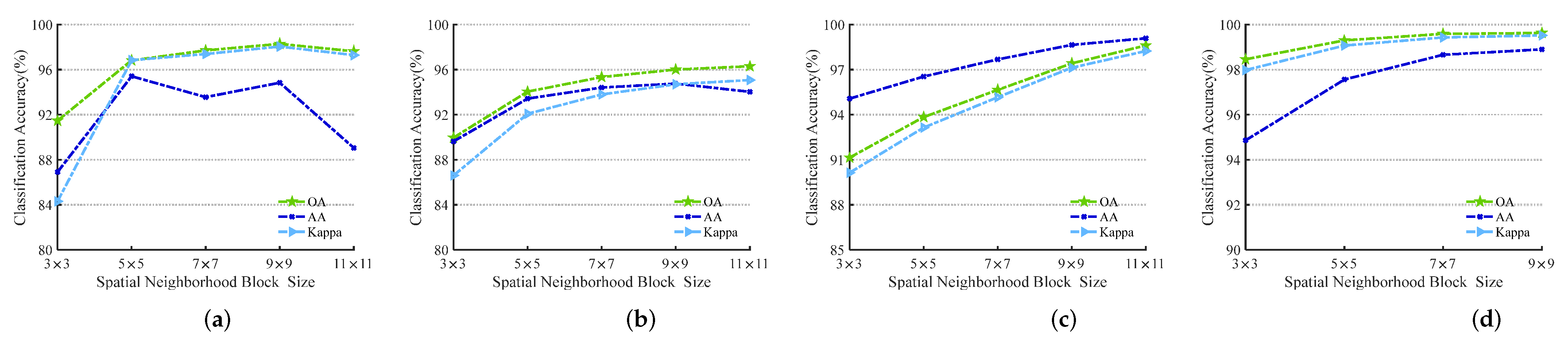
3.3.1. The Influence of Spatial Neighborhood Block Size s

Different sizes of spatial neighborhood blocks size s have a degree of influence on our proposed IFormer method. Therefore, we set the range of spatial neighborhood sizes to 3 × 3, 5 × 5, 7 × 7, 9 × 9, and 11 × 11. In this case, the LK dataset was too large, resulting in insufficient memory for the calculation, so the spatial neighborhood block size was not set to 11 × 11. Figure 11 illustrates the results for the spatial neighborhood blocks in the IP, UP, SV, and LK datasets. With the increase in the spatial neighborhood block size, the three evaluation metrics OA, AA, and Kappa of the IP dataset show a trend of first increasing and then decreasing, so the spatial neighborhood size of the IP dataset is fixed to 9 × 9. The UP, SV, and LK datasets are relatively larger scenes than the IP dataset, and as can be seen in Figure 11, the larger the spatial neighborhood size, the larger the evaluation criteria, so both the UP and SV datasets are set to 11 × 11, while the LK dataset is set to 9 × 9.

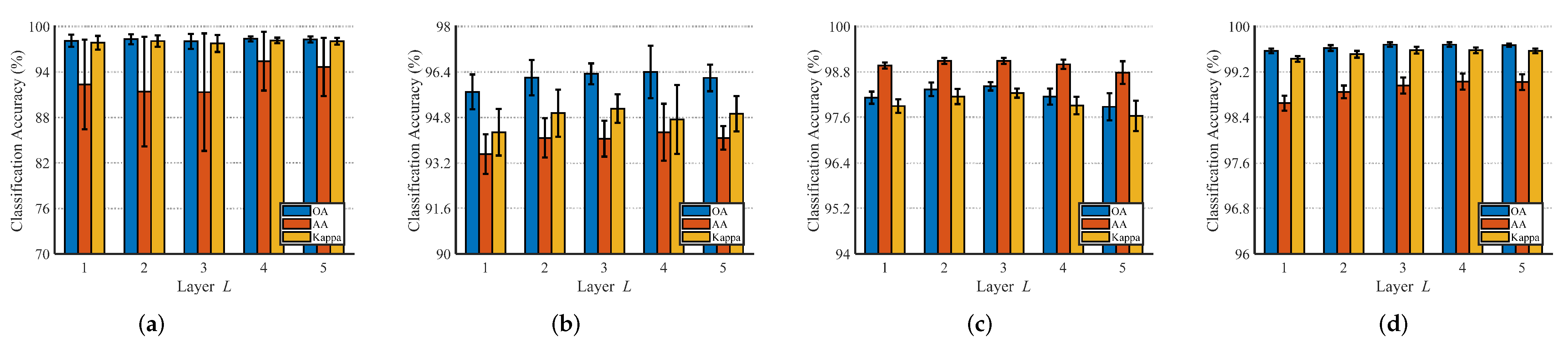
3.3.2. Analysis of the Layer L of the Inception Transformer

The layer of the Inception Transformer has a significant impact on the performance of the IFormer network, and generally speaking, an increase in layer does not necessarily increase performance, but rather, decreases it. Therefore, it is important to choose an appropriate network layer to ensure the robustness of the network. For the four datasets, we set the layers L = 1, 2, 3, 4, and 5 to evaluate the performance of the IFormer method at different layers. In this subsection of the analysis of layer L, we use not only three evaluation indices, as well as the standard deviations of OA, AA, and Kappa as evaluations of IFormer. The performance results of IFormer on the IP and LK datasets (see Figure 12) revealed that OA and Kappa fluctuated less as the number of layers deepened, while AA fluctuated more and gradually increased, with a higher sensitivity to the deepening of the Inception Transformer network layers; therefore, the number of Inception Transformer network layers on the IP and LK datasets was set to 4. IFormer performed best on the UP and SV datasets when the layer was 3 for all three metrics. This is especially true for the UP dataset, probably because the UP dataset features are scattered and small, and the deepening of the network is not conducive to feature identification, so that the network layer is fixed at 3 for the UP and SV datasets.

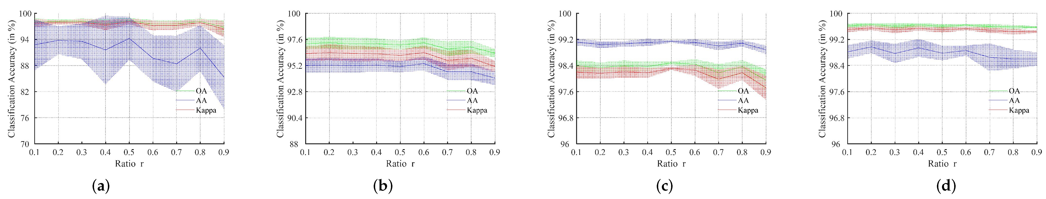
3.3.3. Analysis of the Ratio r of High-Frequency Information to Low-Frequency Information

We adopted a channel splitting mechanism and introduced a channel ratio as a way to better balance the ratio r of high- and low-frequency components in HSI. The four datasets in Figure 13 will be scaled at 0.1 intervals, taken from 0.1 to 0.9, to select high- and low-frequency information. As the proportion of channels rises, the classification accuracy of the IP, UP, and SV datasets exhibit a decrease, a phenomenon that may occur because the inability to focus too much on high-frequency information or low-frequency information can lead to the neglect of global information or local detail considerations. In contrast, on the LK dataset, changes in ratio have a more consistent effect on classification accuracy, due to the distribution of landcovers on the LK dataset, most of which are large scale and simple in structure. Therefore, we fixed the ratio of the four datasets at 0.5 in all experiments.

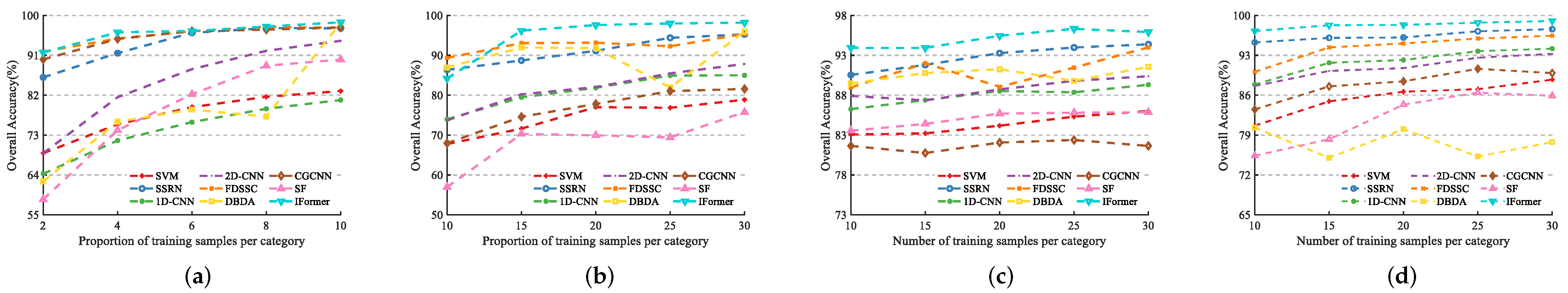
3.4. Analysis of the Role of Different Training Samples on the Classification Effect of the Proposed Method and the Comparison Algorithm

In order to compare the performance of the proposed method IFormer with other state-of-the-art methods under different training samples, Figure 14 shows the performance of the proposed method IFormer. Considering the reasons for the unbalanced sample in the IP dataset, 2%, 4%, 6%, 8%, and 10% were selected according to the proportional distribution of each category. The remaining three datasets had large sample sizes, so training samples were selected at intervals of 5, from 10 per class to 30 per class, respectively. In the beginning, all OAs in the four datasets increased with the training samples. However, when the number of training samples increases, most methods reach a maximum or fluctuate, and DBDA, in particular, is heavily influenced by the training samples. Figure 14 demonstrates that although the recognition accuracy of most algorithms remains constant once the required number of training samples is reached, IFormer remains more competitive than the other algorithms as the training samples increase and the classification accuracy continues to increase.

3.5. Comparing the Training Times and Testing Time Consumptions of Different Algorithms

The average training time and average test time after 10 executions of all compared methods and the proposed method IFormer are recorded in

Table 9. Comparing the computational cost consumption of different methods with the proposed method on four HSI datasets.

Dataset	Evaluations	Calculated Cost Consumption of the Comparison Method and the Proposed Method (in s)
		SVM	SSRN	1D-CNN	2D-CNN	FDSSC	DBDA	CGCNN	SF	IFormer
IP	Training	0.16	4299	161.15	216.84	10,196.12	1583.52	459.91	142.31	121.85
	Test	3.52	38.25	1.07	1.34	49.93	63.56	1.52	1.86	0.86
UP	Training	0.01	2116.45	137.98	159.84	5484.60	432.94	947.43	204.32	51.88
	Test	5.34	117.82	4.29	1.14	188.71	190.39	4.28	7.77	4.19
SV	Training	0.03	1370.59	180.3	261.4	7188.72	710.25	353.74	374.46	65.98
	Test	6.95	109.85	1.21	1.73	322.42	411.31	3.83	9.62	5.75
LK	Training	0.18	10433.04	682.89	1099.33	16,044.62	3144.63	1623.79	1809.78	281.09
	Test	26.99	936.83	4.27	8.66	2222.2	2095.54	8.96	24.47	19.65

. Obviously, because deep learning methods have a lot of parameter tuning and forward propagation, SVMs take less time to train. While there are some comparison methods that have similar accuracies to the proposed method IFormer, the comparison methods have higher training and testing costs, particularly for methods such as FDSSC and DBDA, which may be due to the increased focus on detail, resulting in an increased cost to time. The 1D-CNN and 2D-CNN have less testing time but do not make sufficient use of the HSI features, so the accuracy is low. Although SF has some advantages in training time and testing time on the four datasets, it does not distinguish the feature characteristics well enough to obtain better classification results. Further, the IFormer is competitive in terms of training time and testing time within the allowed range, and still has some advantages for the classification of landcover.

3.6. Analyzing the Impact of the Ghost Module and Inception Transformer on the IFormer Network

To fully verify whether the Ghost Module and Inception Transformer modules behave in IFormer, we therefore conducted ablation experiments on the four datasets shown in

Table 10. Analysis of the effect of Ghost module and Inception Transformer to affect the OA of IFormer on HSI dataset. ✓ means use of the module.

Ghost Module	Inception Transformer	IP	UP	SV	LK
		88.94(2.11)	84.80(1.54)	89.66(1.12)	97.82(0.37)
✓		95.83(1.09)	96.92(0.41)	97.21(0.31)	99.29(0.11)
	✓	96.84(0.87)	96.27(0.31)	97.08(0.29)	99.39(0.06)
✓	✓	98.44(0.45)	98.30(0.46)	98.46(0.17)	99.67(0.02)

, without the Ghost Module and Inception Transformer modules, without the Ghost Module, without the Inception Transformer (replacing the original Transformer), and with the proposed method IFormer. Firstly, the results in Table 10 show that OA without the inclusion of two modules exhibits the lowest classification performance on all four datasets. Then, when either of the two modules, Ghost Module and Inception Transformer, is added, there is a more obvious improvement in the classification performance compared to the previous one without the module, which indicates that the Ghost Module can effectively extract and utilize the rich features, while the Inception Transformer pays more attention to the high- and low-frequency information in the extracted feature maps, to some extent. Finally, we can see from the table that IFormer with two modules included has better classification performance and smaller standard deviation on the four HSI datasets, which reflects that using two modules at the same time can both extract the rich features in HSI and fully capture the global and local features in HSI, which further proves that IFormer facilitates the extraction of deeper feature information in HSI, and thus helps the classification performance.

4. Conclusions

To effectively balance both the high- and low-frequency information (i.e., the local and global features) of HSI data, we propose a new IFormer method to improve HSI classification performance, which is implemented using a 1D-CNN convolutional layer for non-linear feature extraction; then, more feature maps are efficiently generated with a plug-and-play Ghost Module. Finally, the Transformer’s perceptual capability over the spectrum is extended using the Inception Transformer encoder simply and efficiently, allowing for more attention to be focused on HSI high- and low-frequency information. Extensive experiments on four datasets demonstrate that the proposed method still provides satisfactory classification results with limited training samples. Since some datasets perform poorly on a single category, we will work on how to improve better classification performance when the samples are unbalanced in HSI, in the future.

References

1. Gevaert, C.M.; Suomalainen, J.; Tang, J.; Kooistra, L. Generation of spectral–temporal response surfaces by combining multispectral satellite and hyperspectral UAV imagery for precision agriculture applications. IEEE J. Sel. Top. Appl. Earth Obs. Remote Sens. 2015, 8, 3140–3146. [Google Scholar] [CrossRef]
2. Noor, S.S.M.; Michael, K.; Marshall, S.; Ren, J.; Tschannerl, J.; Kao, F. The properties of the cornea based on hyperspectral imaging: Optical biomedical engineering perspective. In Proceedings of the 2016 International Conference on Systems, Signals and Image Processing (IWSSIP), Bratislava, Slovakia, 23–25 May 2016; IEEE: Piscataway, NJ, USA, 2016; pp. 1–4. [Google Scholar]
3. Wang, J.; Zhang, L.; Tong, Q.; Sun, X. The Spectral Crust project—Research on new mineral exploration technology. In Proceedings of the 2012 4th Workshop on Hyperspectral Image and Signal Processing: Evolution in Remote Sensing (WHISPERS), Shanghai, China, 4–7 June 2012; IEEE: Piscataway, NJ, USA, 2012; pp. 1–4. [Google Scholar]
4. Fong, A.; Shu, G.; McDonogh, B. Farm to Table: Applications for New Hyperspectral Imaging Technologies in Precision Agriculture, Food Quality and Safety. In Proceedings of the CLEO: Applications and Technology, Optical Society of America, Washington, DC, USA, 10–15 May 2020; p. AW3K-2. [Google Scholar]
5. Ardouin, J.P.; Lévesque, J.; Rea, T.A. A demonstration of hyperspectral image exploitation for military applications. In Proceedings of the 2007 10th International Conference on Information Fusion, Quebec, QC, Canada, 9–12 July 2007; IEEE: Piscataway, NJ, USA, 2007; pp. 1–8. [Google Scholar]
6. Bioucas-Dias, J.M.; Plaza, A.; Camps-Valls, G.; Scheunders, P.; Nasrabadi, N.; Chanussot, J. Hyperspectral remote sensing data analysis and future challenges. IEEE Geosci. Remote Sens. Mag. 2013, 1, 6–36. [Google Scholar] [CrossRef]
7. Sun, L.; He, C.; Zheng, Y.; Tang, S. SLRL4D: Joint Restoration of Subspace Low-Rank Learning and Non-Local 4-D Transform Filtering for Hyperspectral Image. Remote Sens. 2020, 12, 2979. [Google Scholar] [CrossRef]
8. He, C.; Sun, L.; Huang, W.; Zhang, J.; Zheng, Y.; Jeon, B. TSLRLN: Tensor subspace low-rank learning with non-local prior for hyperspectral image mixed denoising. Signal Process. 2021, 184, 108060. [Google Scholar] [CrossRef]
9. Sun, L.; Wu, F.; Zhan, T.; Liu, W.; Wang, J.; Jeon, B. Weighted nonlocal low-rank tensor decomposition method for sparse unmixing of hyperspectral images. IEEE J. Sel. Top. Appl. Earth Obs. Remote Sens. 2020, 13, 1174–1188. [Google Scholar] [CrossRef]
10. Tu, B.; Yang, X.; Ou, X.; Zhang, G.; Li, J.; Plaza, A. Ensemble entropy metric for hyperspectral anomaly detection. IEEE Trans. Geosci. Remote Sens. 2021, 60, 1–17. [Google Scholar] [CrossRef]
11. Yang, B.; Qin, L.; Liu, J.; Liu, X. UTRNet: An Unsupervised Time-Distance-Guided Convolutional Recurrent Network for Change Detection in Irregularly Collected Images. IEEE Trans. Geosci. Remote Sens. 2022, 60, 1–16. [Google Scholar] [CrossRef]
12. Yang, S.; Shi, Z. Hyperspectral image target detection improvement based on total variation. IEEE Trans. Image Process. 2016, 25, 2249–2258. [Google Scholar] [CrossRef]
13. Tu, B.; Ren, Q.; Zhou, C.; Chen, S.; He, W. Feature Extraction Using Multidimensional Spectral Regression Whitening for Hyperspectral Image Classification. IEEE J. Sel. Top. Appl. Earth Obs. Remote Sens. 2021, 14, 8326–8340. [Google Scholar] [CrossRef]
14. Ren, Q.; Tu, B.; Li, Q.; He, W.; Peng, Y. Multiscale Adaptive Convolution for Hyperspectral Image Classification. IEEE J. Sel. Top. Appl. Earth Obs. Remote Sens. 2022, 15, 5115–5130. [Google Scholar] [CrossRef]
15. Sun, L.; Ma, C.; Chen, Y.; Shim, H.J.; Wu, Z.; Jeon, B. Adjacent superpixel-based multiscale spatial-spectral kernel for hyperspectral classification. IEEE J. Sel. Top. Appl. Earth Obs. Remote Sens. 2019, 12, 1905–1919. [Google Scholar] [CrossRef]
16. Cariou, C.; Chehdi, K. A new k-nearest neighbor density-based clustering method and its application to hyperspectral images. In Proceedings of the 2016 IEEE International Geoscience and Remote Sensing Symposium (IGARSS), Beijing, China, 10–15 July 2016; IEEE: Piscataway, NJ, USA, 2016; pp. 6161–6164. [Google Scholar]
17. SahIn, Y.E.; Arisoy, S.; Kayabol, K. Anomaly detection with Bayesian Gauss background model in hyperspectral images. In Proceedings of the 2018 26th Signal Processing and Communications Applications Conference (SIU), Izmir, Turkey, 2–5 May 2018; IEEE: Piscataway, NJ, USA, 2018; pp. 1–4. [Google Scholar]
18. Paoletti, M.E.; Haut, J.M.; Plaza, J.; Plaza, A. Deep&dense convolutional neural network for hyperspectral image classification. Remote Sens. 2018, 10, 1454. [Google Scholar]
19. Chen, Y.N.; Thaipisutikul, T.; Han, C.C.; Liu, T.J.; Fan, K.C. Feature line embedding based on support vector machine for hyperspectral image classification. Remote Sens. 2021, 13, 130. [Google Scholar] [CrossRef]
20. Zhou, C.; Tu, B.; Ren, Q.; Chen, S. Spatial peak-aware collaborative representation for hyperspectral imagery classification. IEEE Geosci. Remote Sens. Lett. 2021, 19, 1–5. [Google Scholar] [CrossRef]
21. Peng, J.; Sun, W.; Li, H.C.; Li, W.; Meng, X.; Ge, C.; Du, Q. Low-rank and sparse representation for hyperspectral image processing: A review. IEEE Geosci. Remote Sens. Mag. 2022, 10, 10–43. [Google Scholar] [CrossRef]
22. Prasad, S.; Bruce, L.M. Limitations of principal components analysis for hyperspectral target recognition. IEEE Geosci. Remote Sens. Lett. 2008, 5, 625–629. [Google Scholar] [CrossRef]
23. Villa, A.; Benediktsson, J.A.; Chanussot, J.; Jutten, C. Hyperspectral image classification with independent component discriminant analysis. IEEE Trans. Geosci. Remote Sens. 2011, 49, 4865–4876. [Google Scholar] [CrossRef]
24. Fu, L.; Li, Z.; Ye, Q.; Yin, H.; Liu, Q.; Chen, X.; Fan, X.; Yang, W.; Yang, G. Learning robust discriminant subspace based on joint L2, p-and L2, s-norm distance metrics. IEEE Trans. Neural Netw. Learn. Syst. 2022, 33, 130–144. [Google Scholar] [CrossRef]
25. Fauvel, M.; Benediktsson, J.A.; Chanussot, J.; Sveinsson, J.R. Spectral and spatial classification of hyperspectral data using SVMs and morphological profiles. IEEE Trans. Geosci. Remote Sens. 2008, 46, 3804–3814. [Google Scholar] [CrossRef]
26. Benediktsson, J.A.; Palmason, J.A.; Sveinsson, J.R. Classification of hyperspectral data from urban areas based on extended morphological profiles. IEEE Trans. Geosci. Remote Sens. 2005, 43, 480–491. [Google Scholar] [CrossRef]
27. Dalla Mura, M.; Villa, A.; Benediktsson, J.A.; Chanussot, J.; Bruzzone, L. Classification of hyperspectral images by using extended morphological attribute profiles and independent component analysis. IEEE Geosci. Remote Sens. Lett. 2010, 8, 542–546. [Google Scholar] [CrossRef] [Green Version]
28. Chen, Y.; Lin, Z.; Zhao, X.; Wang, G.; Gu, Y. Deep learning-based classification of hyperspectral data. IEEE J. Sel. Top. Appl. Earth Obs. Remote Sens. 2014, 7, 2094–2107. [Google Scholar] [CrossRef]
29. Chen, Y.; Zhao, X.; Jia, X. Spectral–spatial classification of hyperspectral data based on deep belief network. IEEE J. Sel. Top. Appl. Earth Obs. Remote Sens. 2015, 8, 2381–2392. [Google Scholar] [CrossRef]
30. He, K.; Zhang, X.; Ren, S.; Sun, J. Deep residual learning for image recognition. In Proceedings of the IEEE Conference on Computer Vision and Pattern Recognition, Las Vegas, NV, USA, 27–30 June 2016; pp. 770–778. [Google Scholar]
31. Hu, W.; Huang, Y.; Wei, L.; Zhang, F.; Li, H. Deep convolutional neural networks for hyperspectral image classification. J. Sens. 2015, 2015, 258619. [Google Scholar] [CrossRef]
32. Zhao, W.; Du, S. Spectral–spatial feature extraction for hyperspectral image classification: A dimension reduction and deep learning approach. IEEE Trans. Geosci. Remote Sens. 2016, 54, 4544–4554. [Google Scholar] [CrossRef]
33. Chen, Y.; Jiang, H.; Li, C.; Jia, X.; Ghamisi, P. Deep feature extraction and classification of hyperspectral images based on convolutional neural networks. IEEE Trans. Geosci. Remote Sens. 2016, 54, 6232–6251. [Google Scholar] [CrossRef]
34. Liu, Q.; Xiao, L.; Yang, J.; Chan, J.C.W. Content-guided convolutional neural network for hyperspectral image classification. IEEE Trans. Geosci. Remote Sens. 2020, 58, 6124–6137. [Google Scholar] [CrossRef]
35. Zhong, Z.; Li, J.; Luo, Z.; Chapman, M. Spectral–spatial residual network for hyperspectral image classification: A 3-D deep learning framework. IEEE Trans. Geosci. Remote Sens. 2017, 56, 847–858. [Google Scholar] [CrossRef]
36. Wang, W.; Dou, S.; Jiang, Z.; Sun, L. A fast dense spectral–spatial convolution network framework for hyperspectral images classification. Remote Sens. 2018, 10, 1068. [Google Scholar] [CrossRef]
37. Ma, W.; Yang, Q.; Wu, Y.; Zhao, W.; Zhang, X. Double-branch multi-attention mechanism network for hyperspectral image classification. Remote Sens. 2019, 11, 1307. [Google Scholar] [CrossRef]
38. Li, R.; Zheng, S.; Duan, C.; Yang, Y.; Wang, X. Classification of hyperspectral image based on double-branch dual-attention mechanism network. Remote Sens. 2020, 12, 582. [Google Scholar] [CrossRef] [Green Version]
39. Beal, J.; Kim, E.; Tzeng, E.; Park, D.H.; Zhai, A.; Kislyuk, D. Toward transformer-based object detection. arXiv 2020, arXiv:2012.09958. [Google Scholar]
40. Fang, Y.; Liao, B.; Wang, X.; Fang, J.; Qi, J.; Wu, R.; Niu, J.; Liu, W. You only look at one sequence: Rethinking transformer in vision through object detection. Adv. Neural Inf. Process. Syst. 2021, 34, 26183–26197. [Google Scholar]
41. Zheng, S.; Lu, J.; Zhao, H.; Zhu, X.; Luo, Z.; Wang, Y.; Fu, Y.; Feng, J.; Xiang, T.; Torr, P.H.; et al. Rethinking semantic segmentation from a sequence-to-sequence perspective with transformers. In Proceedings of the IEEE Conference on Computer Vision and Pattern Recognition, Nashville, TN, USA, 19–25 June 2021; pp. 6881–6890. [Google Scholar]
42. Xie, E.; Wang, W.; Yu, Z.; Anandkumar, A.; Alvarez, J.M.; Luo, P. SegFormer: Simple and efficient design for semantic segmentation with transformers. Adv. Neural Inf. Process. Syst. 2021, 34, 12077–12090. [Google Scholar]
43. He, X.; Chen, Y.; Lin, Z. Spatial-spectral transformer for hyperspectral image classification. Remote Sens. 2021, 13, 498. [Google Scholar] [CrossRef]
44. Qing, Y.; Liu, W.; Feng, L.; Gao, W. Improved transformer net for hyperspectral image classification. Remote Sens. 2021, 13, 2216. [Google Scholar] [CrossRef]
45. Hong, D.; Han, Z.; Yao, J.; Gao, L.; Zhang, B.; Plaza, A.; Chanussot, J. SpectralFormer: Rethinking hyperspectral image classification with transformers. IEEE Trans. Geosci. Remote Sens. 2021, 60, 1–15. [Google Scholar] [CrossRef]
46. Kauffmann, L.; Ramanoël, S.; Peyrin, C. The neural bases of spatial frequency processing during scene perception. Front. Integr. Neurosci. 2014, 8, 37. [Google Scholar] [CrossRef]
47. Dosovitskiy, A.; Beyer, L.; Kolesnikov, A.; Weissenborn, D.; Zhai, X.; Unterthiner, T.; Dehghani, M.; Minderer, M.; Heigold, G.; Gelly, S.; et al. An image is worth 16x16 words: Transformers for image recognition at scale. arXiv 2020, arXiv:2010.11929. [Google Scholar]
48. Han, K.; Wang, Y.; Tian, Q.; Guo, J.; Xu, C.; Xu, C. Ghostnet: More features from cheap operations. In Proceedings of the IEEE Conference on Computer Vision and Pattern Recognition, Seattle, WA, USA, 14–19 June 2020; pp. 1580–1589. [Google Scholar]
49. Si, C.; Yu, W.; Zhou, P.; Zhou, Y.; Wang, X.; Yan, S. Inception Transformer. arXiv 2022, arXiv:2205.12956. [Google Scholar]
50. Zhong, Y.; Hu, X.; Luo, C.; Wang, X.; Zhao, J.; Zhang, L. WHU-Hi: UAV-borne hyperspectral with high spatial resolution (H2) benchmark datasets and classifier for precise crop identification based on deep convolutional neural network with CRF. Remote Sens. Environ. 2020, 250, 112012. [Google Scholar] [CrossRef]
51. Zhong, Y.; Wang, X.; Xu, Y.; Wang, S.; Jia, T.; Hu, X.; Zhao, J.; Wei, L.; Zhang, L. Mini-UAV-borne hyperspectral remote sensing: From observation and processing to applications. IEEE Geosci. Remote Sens. Mag. 2018, 6, 46–62. [Google Scholar] [CrossRef]
52. Melgani, F.; Bruzzone, L. Classification of hyperspectral remote sensing images with support vector machines. IEEE Trans. Geosci. Remote Sens. 2004, 42, 1778–1790. [Google Scholar] [CrossRef]
53. Chang, C.C.; Lin, C.J. LIBSVM: A library for support vector machines. ACM Trans. Intell. Syst. Technol. 2011, 2, 1–27. [Google Scholar] [CrossRef]
54. Li, Y.; Zhang, H.; Shen, Q. Spectral–spatial classification of hyperspectral imagery with 3D convolutional neural network. Remote Sens. 2017, 9, 67. [Google Scholar] [CrossRef]
55. Gao, H.; Lin, S.; Yang, Y.; Li, C.; Yang, M. Convolution neural network based on two-dimensional spectrum for hyperspectral image classification. J. Sens. 2018, 2018, 8602103. [Google Scholar] [CrossRef] [Green Version]
56. Huang, G.; Liu, Z.; Van Der Maaten, L.; Weinberger, K.Q. Densely connected convolutional networks. In Proceedings of the IEEE Conference on Computer Vision and Pattern Recognition, Honolulu, HI, USA, 21–26 July 2017; pp. 4700–4708. [Google Scholar]
57. Fu, J.; Liu, J.; Tian, H.; Li, Y.; Bao, Y.; Fang, Z.; Lu, H. Dual attention network for scene segmentation. In Proceedings of the IEEE Conference on Computer Vision and Pattern Recognition, Long Beach, CA, USA, 15–20 June 2019; pp. 3146–3154. [Google Scholar]
Figure 1. The structure of the proposed IFormer. ϕ represents the cheap operation and ⨁ denotes the concatenate operations.
Remotesensing 14 04866 g001
Figure 2. Structure diagram of the Inception token mixer in Inception Transformer.
Remotesensing 14 04866 g002
Figure 3. IP dataset. (a) Composite image. (b) Training set. (c) Test set. (d) Legend.
Remotesensing 14 04866 g003
Figure 4. UP dataset. (a) Composite image. (b) Training set. (c) Test set. (d) Legend.
Remotesensing 14 04866 g004
Figure 5. SV dataset. (a) Composite image. (b) Training set. (c) Test set. (d) Legend.
Remotesensing 14 04866 g005
Figure 6. LK dataset. (a) Composite image. (b) Training set. (c) Test set. (d) Legend.
Remotesensing 14 04866 g006
Figure 7. Classification results of ground truth and comparison methods for the IP dataset. (a) Ground Truth. (b) SVM. (c) SSRN. (d) 1D-CNN. (e) 2D-CNN. (f) FDSSC. (g) DBDA. (h) CECNN. (i) SF. (j) IFormer.
Remotesensing 14 04866 g007
Figure 8. Classification results of ground truth and comparison methods for the UP dataset. (a) Ground Truth. (b) SVM. (c) SSRN. (d) 1D-CNN. (e) 2D-CNN. (f) FDSSC. (g) DBDA. (h) CECNN. (i) SF. (j) IFormer.
Remotesensing 14 04866 g008
Figure 9. Classification results of ground truth and comparison methods for the SV dataset. (a) Ground Truth. (b) SVM. (c) SSRN. (d) 1D-CNN. (e) 2D-CNN. (f) FDSSC. (g) DBDA. (h) CECNN. (i) SF. (j) IFormer.
Remotesensing 14 04866 g009
Figure 10. Classification results of ground truth and comparison methods for the LK dataset. (a) Ground Truth. (b) SVM. (c) SSRN. (d) 1D-CNN. (e) 2D-CNN. (f) FDSSC. (g) DBDA. (h) CECNN. (i) SF. (j) IFormer.
Remotesensing 14 04866 g010
Figure 11. The impact of input spatial neighborhood block size on network performance. (a) Indian Pines dataset. (b) Universit of Pavia dataset. (c) Salinas dataset. (d) Long Kou dataset.
Remotesensing 14 04866 g011
Figure 12. Effect of Inception Transformer’s layer L on the performance of IFormer network structures. (a) Indian Pines dataset. (b) Universit of Pavia dataset. (c) Salinas dataset. (d) Long Kou dataset.
Remotesensing 14 04866 g012
Figure 13. The influence of the ratio r of high-frequency channels to low-frequency channels on the performance of IFormer networks. The margin of error is expressed as the standard deviation of the evaluation index. (a) Indian Pines dataset. (b) University of Pavia dataset. (c) Salinas dataset. (d) Long Kou dataset.
Remotesensing 14 04866 g013
Figure 14. Performance of our proposed method and comparison methods on different datasets with different training samples. (a) Indian Pines dataset. (b) University of Pavia dataset. (c) Salinas dataset. (d) Long Kou dataset.
Remotesensing 14 04866 g014