Classification of Ground-Based Cloud Images by Contrastive Self-Supervised Learning

Abstract

Clouds have an enormous influence on the hydrological cycle, Earth’s radiation budget, and climate changes. Accurate automatic recognition of cloud shape based on ground-based cloud images is beneficial to analyze the atmospheric motion state and water vapor content, and then to predict weather trends and identify severe weather processes. Cloud type classification remains challenging due to the variable and diverse appearance of clouds. Deep learning-based methods have improved the feature extraction ability and the accuracy of cloud type classification, but face the problem of lack of labeled samples. In this paper, we proposed a novel classification approach of ground-based cloud images based on contrastive self-supervised learning (CSSL) to reduce the dependence on the number of labeled samples. First, data augmentation is applied to the input data to obtain augmented samples. Then contrastive self-supervised learning is used to pre-train the deep model with a contrastive loss and a momentum update-based optimization. After pre-training, a supervised fine-tuning procedure is adopted on labeled data to classify ground-based cloud images. Experimental results have confirmed the effectiveness of the proposed method. This study can provide inspiration and technical reference for the analysis and processing of other types of meteorological remote sensing data under the scenario of insufficient labeled samples.

1. Introduction

In meteorological observation, cloud analysis plays a crucial role since clouds affect the hydrological cycle, Earth’s radiation budget, and climate changes [1,2,3,4]. Cloud observation can mainly be divided into two categories: satellite-based [5,6,7] and ground-based [8,9,10]. The satellite remote sensing observation aims to monitor the distribution, movement and change of clouds over large areas from a downward viewpoint. However, satellite observation cannot provide sufficient spatial and temporal resolutions to describe detailed cloud characteristics over a particular area [10,11]. On the other hand, the ground-based cloud observation open up new opportunities for monitoring and understanding regional sky conditions [10]. In comparison with satellite images of clouds, ground-based cloud images are mainly used to observe local sky areas, with higher temporal and spatial resolution. Typical ground-based remote sensing observation instruments include Total Sky Imager (TSI) [12], Whole Sky Imager (WSI) [13,14], and All Sky Imager (ASI) [15,16]. Figure 1 shows the pictures of typical TSI and ASI. What they observe is the information at the bottom of the cloud, and the cloud features are more obvious, which is more conducive to assisting the weather forecast in local areas [17]. For example, using the data obtained from ground-based equipment, forecasters can judge the types of clouds and then analyze the weather change trend (e.g., stratus clouds usually indicate a sunny day, while cumulonimbus capillatus clouds indicate thunderstorm weather). Therefore, the ground-based method plays an irreplaceable role in cloud observation at a local scale.

Cloud observation involves three main aspects, i.e., height, coverage, and type [10], which are important reference data for analyzing sky conditions and forecasting short-term weather. Among them, cloud types are mainly reflected in the form of cloud shapes. With the advancement of cloud measurement equipment, the observation of cloud height and cloud coverage by the meteorological department has achieved instrumental measurement and can ensure high reliability, while the observation and identification of cloud shapes is still dominated by manual observation. The cloud shape reflects the physical properties of the cloud to a certain extent, and its change and development are an effective representation of the atmospheric motion state [18,19]. Accurate automatic recognition of cloud shape based on ground-based cloud images is beneficial to continuously obtain cloud shape information, analyze atmospheric motion state and water vapor content, etc., and then predict weather trends and identify severe weather processes [11].

With the development of ground-based remote sensing observation instruments, a large amount of cloud images are collected. The data from these imaging devices provide preconditions for research on automatic cloud classification. Essentially, cloud type classification using ground-based cloud images is the specific application of pattern recognition technology in the field of cloud observation. Its main task is to classify each cloud image captured from ground into the corresponding cloud category, such as stratus, cumulus, cirrus, cumulonimbus, etc.

Early research on ground-based image classification relied on manual classification methods, which focused on features such as texture, structure and color features in conjunction with traditional machine learning methods to classify ground-based cloud images. These methods include decision tree, K-nearest neighbors (KNN) classifier, support vector machine (SVM), extreme learning machine (ELM), linear discriminant analysis (LDA), etc. Buch et al. [20] used LAWS texture, pixel location and pixel brightness to describe different clouds, and used a binary decision tree as a classifier for classification. On this basis, Singh et al. [21] combined several other forms of texture information, such as autocorrelation, co-occurrence matrices, edge frequency, etc., to jointly characterize ground-based cloud images, and compared the classification ability of three classifiers (KNN, linear classifier, neural network). The statistical texture features and pattern features using Fourier spectrum are employed in Calbó et al [8], where a threshold-based method is used for classification. Heinle et al. [22] proposed to describe the cloud image using spectral features (mean, standard deviation, skewness, and difference) and texture features (energy, entropy, contrast, homogenity, and cloud cover). Combined with the KNN classifier, the ground-based cloud images were divided into seven categories. Liu et al. [23] studied the classification of near-infrared ground-based cloud images, using features including gray mean value, cloud fraction, edge sharpness, and cloud mass and gap distribution parameters. Isosalo et al. [24] compared the performance of local binary pattern (LBP) and local edge pattern (LEP) features, using KNN as the classifier, and pointed out that LBP features are more suitable for ground-based cloud image classification. On this basis, Refs. [25,26] proposed saliency LBP and stable LBP, respectively, as features for ground-based cloud image classification, and the classifiers used were the nearest neighbor classifier, SVM and multilayer perceptron (MLP), respectively. In addition, Oikonomou et al. [27] used regional LBP to take into account both global and local textural information from cloud type patterns to improve the classification accuracy, where a linear SVM and LDA classifiers are adopted in the classification stage. Zhuo et al. [28] proposed that the spatial distribution of contours can represent the structural information of cloud shapes, and used the CENTRIST descriptor pyramid to simultaneously extract the texture and structural features of the ground-based cloud images, and used SVM and KNN to classify the cloud image. Li et al. [29] characterized the ground-based cloud image by establishing a bag of micro-structures, and combined SVM to classify the cloud images into five categories. It can be seen that the traditional machine learning-based cloud recognition method for ground-based cloud images mainly uses hand-designed features such as texture, structure, color, and shape, and obtains high-dimensional feature expressions of ground-based cloud images through a single feature or a combination of multiple descriptors. Most of these methods start from the point of view of digital signal analysis and mathematical statistical characteristics in feature description, but ignore the representation and interpretation of the visual characteristics of the image itself. However, as a result of cloud appearance variability and diversity, it is extremely challenging to accurately classify cloud types and the research is still ongoing.

During recent years, deep learning (DL) methods have been widely used in image recognition, object detection, speech recognition, natural language processing and other fields, such as instrumentation and measurement [30,31,32,33,34,35]. The main reason for the success of deep learning technology is that through the deep (hierarchical) structure, it can better perform abstract representation of features and mine invariance in features [36]. With the in-depth integration of artificial intelligence and meteorological data processing technology, deep learning-based solutions continue to heat up in the meteorological field [37,38]. At present, there are some works that combine deep learning with ground-based cloud type recognition. The deep models adopted include convolutional neural networks (CNN) [17,39,40,41,42] and graph neural networks (GNN) [4,10,43]. Ye et al. [39] took the lead in introducing the deep learning model into the cloud type recognition of ground-based cloud images, and proposed an extraction method of high-level semantic features of ground cloud images using convolutional neural networks (CNN). On this basis, they combined Fisher vector (FV) coding and SVM for cloud classification of ground-based cloud images. Subsequently, the author extended this work and proposed a cloud recognition method based on multi-layer semantic feature mining using CNN model in [17], which screened out local patterns with strong discriminative ability from multiple convolutional layers of CNN model, and encodes local convolutional features in the form of Fisher vectors to achieve simultaneous extraction of multi-scale and multi-level features of ground-based cloud images. In [40,41,42], CNN is also used for ground-based cloud image classification, and the classical network structure of multi-layer convolution and max-pooling operation is adopted. Liu et al. [44] combined the multi-modal information (temperature, air pressure, humidity, wind speed, etc.) with the visual features of the ground-based cloud image extracted by CNN, so as to improve the accuracy and robustness of the ground cloud image cloud classification. Furthermore, Ref. [45] added an attentive network on the basis of [44] to further explore local visual features of ground-based cloud images.

In addition to the most commonly used CNN model in computer vision, researchers also introduced other new deep learning models, such as graph neural networks (GNN), into classification of ground-based cloud images. Liu et al. [10] applied a commonly used GNN model, graph convolutional networks (GCN), to the feature extraction of ground-based cloud images; specifically, the visual features extracted by CNN were taken as nodes of the graph, and the similarity between nodes as edges of the graph, and the network training was conducted through graph representation learning. In [43], multi-modal information such as temperature, air pressure, humidity, and wind speed is incorporated with GCN-based features to further improve the classification accuracy. Ref. [4] proposed a context graph attention network (GAT) for ground-based remote sending cloud classification, where the attention module is introduced to reflect the importance of connected nodes more precisely.

These deep learning-based efforts have improved the feature extraction ability and the accuracy of cloud type classification, but face the problem of lack of labeled samples. The main driving force of deep learning is the amount of available data. However, in the real ground-based cloud image classification scene, it is often difficult to collect a large number of labeled samples. For example, the SWIMCAT dataset, which is commonly used in ground-based cloud image classification research, has a total of 784 images. These images are divided into five cloud categories, and the minimum category has only 85 images. How to perform effective learning on “small sample” ground-based cloud image datasets has become a difficult problem in designing deep learning models.

In recent years, self-supervised learning (SSL) has become a hot research direction of machine learning. The self-supervised learning method is a special form of unsupervised learning method. Its main idea is that data itself provides supervised information for the learning algorithm, which can make full use of a large number of unlabeled data for feature learning [46,47]. Generally, self-supervised learning is divided into two categories: generative learning and contrastive learning [47]. Among them, contrastive self-supervised learning has become a research focus of machine learning in recent two or three years due to its characteristics of simple model and optimization and strong generalization ability. Representative works of contrastive learning include SimCLR [48], MoCo [49], SwAV [50], BYOL [51], etc. Inspired by these works, aiming at the challenge of insufficient labeled samples faced by the existing ground-based cloud images classification methods based on deep learning, this paper proposes a new classification method of ground-based cloud images based on contrastive self-supervised learning (CSSL) to reduce the dependence on the number of labeled samples, improve the representation ability of ground-based cloud images, and improve the classification accuracy. The main contributions of this article are summarized as follows.

• The contrastive self-supervised learning (CSSL) is adopted to learn discriminating features of ground-based cloud images. To the best of our knowledge, this is the first work to utilize a self-supervised learning framework for ground-based remote sensing cloud classification, which provides a new perspective for the better utilization of cloud measuring instruments.
• The deep model learned from CSSL is transferred and serves as the appropriate initial parameters of the fine-tuning procedure. The overall approach integrates the advantages of unsupervised and supervised learning to boost the classification performance.
• The proposed method is demonstrated to outperform several state-of-the-art deep learning-based methods on a real dataset of ground-based cloud images, showing that CSSL is an effective strategy for exploiting the information of unlabeled cloud images.

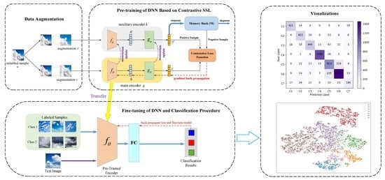
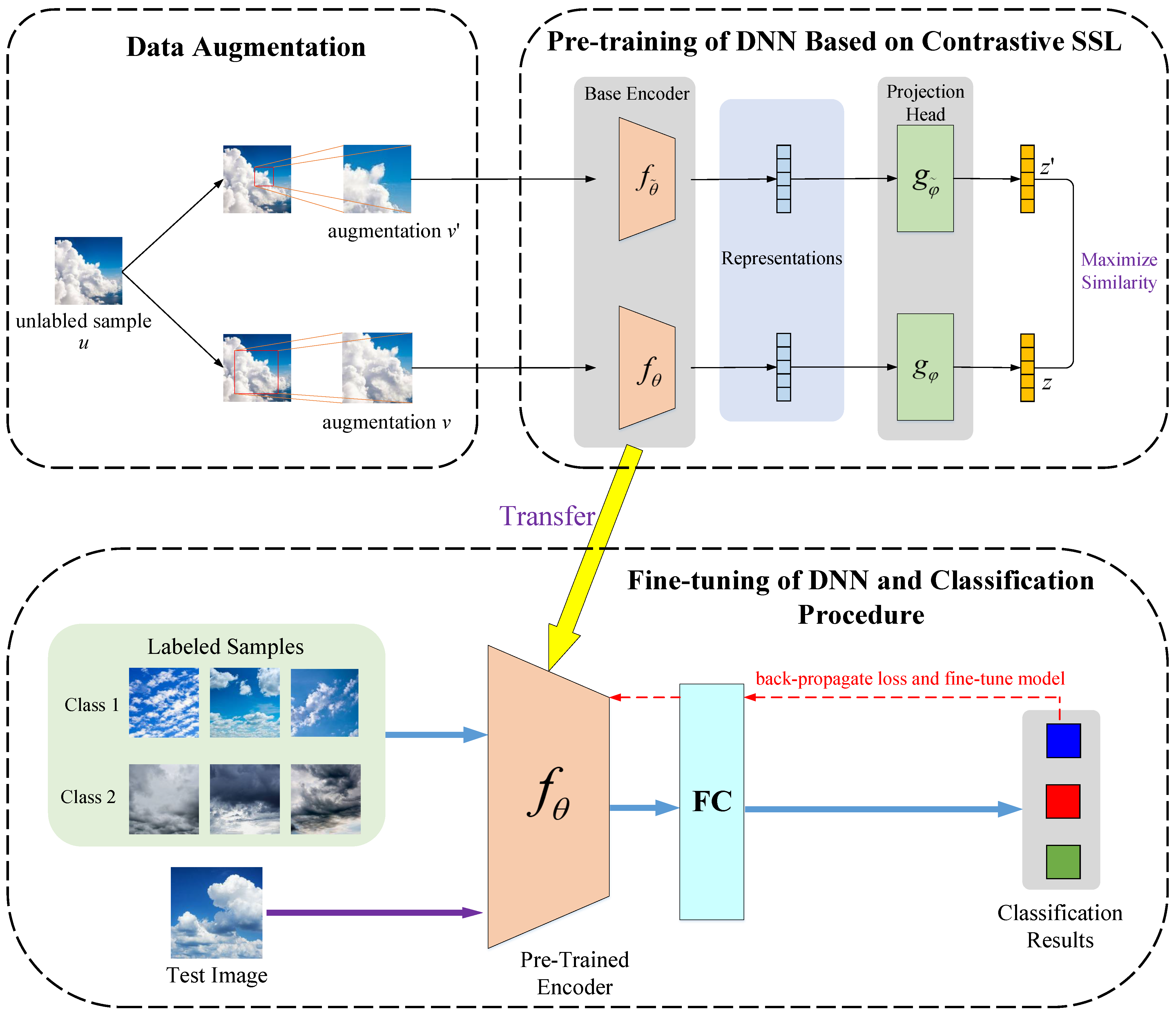
The remainder of this paper is organized as follows. Section 2 describes the proposed CSSL classification method. Section 3 presents the experimental results as well as the details of the experiments. Finally, this study is concluded in Section 5.

2. Method

The method proposed in this paper mainly includes data augmentation, network pre-training based on contrastive self-supervised learning, and fine-tuning of the deep neural networks (DNN). The flowchart is shown in Figure 2.

The data augmentation methods to be used in the article include image rotation, flipping, cropping and resizing, color jittering, random noise, image blurring (such as Gaussian blurring), etc. The augmented cloud image has the same size as the original image. Among them, rotation includes three rotation forms (90°, 180°, and 270°), and flipping includes flipping and vertical flipping. Cropping and resizing is to randomly select an area from the image and resize the area to the size of the original image. Figure 3 shows examples of the effect of four data augmentation methods: cropping and resizing, rotation, random noise, and Gaussian blur. By randomly changing the training samples, the model’s dependence on some attributes can be reduced and the generalization ability of the model can be improved. For example, the image is cropped in different ways so that the target of interest appears in different positions, thereby reducing the model’s dependence on position; random color jittering is performed on the image to reduce the model’s sensitivity to color.

On the basis of data augmentation, contrastive self-supervised learning is used to learn the feature representation of ground-based cloud images. The main process is shown in Figure 4. The learning framework mainly includes main encoder, auxiliary encoder, contrast loss function, memory bank, etc. For the unlabeled sample u, through different data augmentation methods, its two augmented samples v and v’ are obtained. Then, the augmented samples v and v’ are, respectively, passed through the main encoder and the auxiliary encoder to obtain the corresponding embedding vectors, namely z and z’. The main encoder and the auxiliary encoder use the same network structure, but the update methods of the two are different. After that, the framework updates the network by using the contrastive loss function. The memory bank M is mainly used to store negative samples and form negative sample pairs.

The main encoder consists of two parts: the base encoder and the projection head. We adopt the classical residual network ResNet-50 [52] as the base encoder. The data v obtains its feature representation h after passing through the base encoder f, and then it is input into a projection head network g. The projection head plays a role in mapping the feature representation onto the space acted on by the contrastive loss function, and reducing information loss in downstream tasks [48,49]. In this paper, a multilayer perceptron (MLP) is proposed to be used to construct the projection head. We denote the learnable parameter set in the base encoder f and the projection head g by $\theta$ and $\phi$, then f and g are also denoted as $f_{\theta }$ and $g_{\phi }$.

The auxiliary encoder has the same topology and hyperparameters as the main encoder, and its function is to construct sample pairs required to form the contrastive loss function. We use $f_{\tilde{\theta }}$ and $g_{\tilde{\phi }}$ to represent the base encoder and the projection head in the auxiliary encoder, where $\tilde{\theta }$ and $\tilde{\phi }$ are learnable hyperparameters.

As show in Figure 4, the unlabeled sample receives two augmented samples v and v’ through data augmentation, and then v receives the embedding vector z through $f_{\theta }$ and $g_{\phi }$ of the main encoder, i.e., $z=g_{\phi }\left(f_{\theta }\left(v\right)\right)$; meanwhile, v’ receives the embedding vector z’ through $f_{\tilde{\theta }}$ and $g_{\tilde{\phi }}$ of the auxiliary encoder, i.e., $z^{\prime }=g_{\tilde{\phi }}\left(f_{\tilde{\theta }}\left(v^{\prime }\right)\right)$. In self-supervised training, each unlabeled sample is treated as a separate category. z and z’ come from the same unlabeled sample and form a positive sample pair. For convenience of description, z’ is also written as $z^{+}$, indicating that z’ is a positive sample of z.

In the process of contrastive learning, besides positive sample pairs, negative sample pairs are also required. In this paper, negative sample pairs are constructed using the memory bank. In implementation, the memory bank adopts a “first in first out” queue data structure. During the learning process, unlabeled data is input in the form of minibatch. The embedding vector of the sample in a minibatch acquired by the auxiliary encoder will be saved in the memory bank M through the enqueuing operation, and the earliest minibatch in M will be removed from the queue. The negative sample pairs are constructed in such a way that the embedding vector z of the current sample obtained by the main encoder and the embedding vectors corresponding to all previous minibatches that are still in the queue stored in the memory bank M form a negative sample pair. Theoretically, the more negative sample pairs, the better the effect of self supervised learning [49]. Since M can usually be set very large, the number of negative sample pairs can be increased, and the learning effect can be improved by introducing the dynamically updated memory bank.

After the positive and negative sample pairs are constructed, a key issue is to design the contrastive loss function. The goal of this function is to make the sample representation learned as close as possible to the representation of the positive sample and as far as possible from the representation of the negative sample. The InfoNCE [53] contrastive loss function is applied in this paper:

$$\begin{array}{c}\mathcal{L}{}_{pretraining}=-log\frac{exp(sim(z,z_{}^{+})/\tau )}{exp(sim(z,z_{}^{+})/\tau )+{\sum }_{j=1}^{N}exp(sim(z,z_j^{-})/\tau )}\hfill \end{array}$$

(1)

where $z^{+}$ represents the positive sample and $z_j^{-}$ represents the j-th negative sample; N denotes the total number of negative samples that are stored in the memory bank; temperature coefficient $\tau$ is a hyperparameter that controls how uniformly information is distributed [54]. $sim(·,·)$ represents the similarity function, which is the cosine similarity in this paper:

$$\begin{array}{c}sim(z_i,z_j)=\frac{z_i^T{z}_j}{\left|\right|z_i\left|\right|\left|\right|z_j\left|\right|}\hfill \end{array}$$

(2)

By minimizing the loss function in Equation (1), the augmented images from the same original source are pulled together in the feature space, while those from different sources are pushed apart. Thus, the codes of the same type of data tend to be similar, and the data of different types tend to be far away, which is useful for conducting the downstream ground-based cloud image categorization task. The loss function is back-propagated to update the network parameters of the main encoder (i.e., the parameters $\theta$ of the base encoder and and $\phi$ of the projection head) through the stochastic gradient descent (SGD) algorithm, as shown by the red dotted line in Figure 4.

For the sake of consistency, the parameters of $\tilde{\theta }$ and $\tilde{\phi }$ in the auxiliary encoder are not directly updated with the loss function by back-propagation. Inspired by [49], we update the auxiliary encoder’s network parameters $\tilde{\theta }$ and $\tilde{\phi }$ with a momentum-based strategy:

$$\begin{array}{c}\left\{\begin{array}{c}\tilde{\theta }\leftarrow m\tilde{\theta }+(1-m)\theta \hfill \\ \tilde{\phi }\leftarrow m\tilde{\phi }+(1-m)\phi \hfill \end{array}\right.\hfill \end{array}$$

(3)

where m represents the momentum coefficient and is in the range of 0 and 1. The value of m is generally selected to be relatively large (above 0.99) to make the update of the auxiliary encoder more smooth and stable. The momentum update process is shown by the purple dashed line in Figure 4.

After pre-training, a supervised fine-tuning process is required for the classification task. The pre-trained base encoder $f_{\theta }$ of the main encoder is transferred for the representation learning of labeled training samples. A trainable fully-connected (FC) layer is connected behind $f_{\theta }$. The parameters in $f_{\theta }$ and FC are fine-tuned through back-propagation.

When the architecture and weights of deep model are specified, the fine-tuned model can be used to classify ground-based cloud images using a forward-propagation step. In the output layer of FC, the node index corresponding to the largest value is considered to be the current image’s predicted label.

3. Experiments and Results

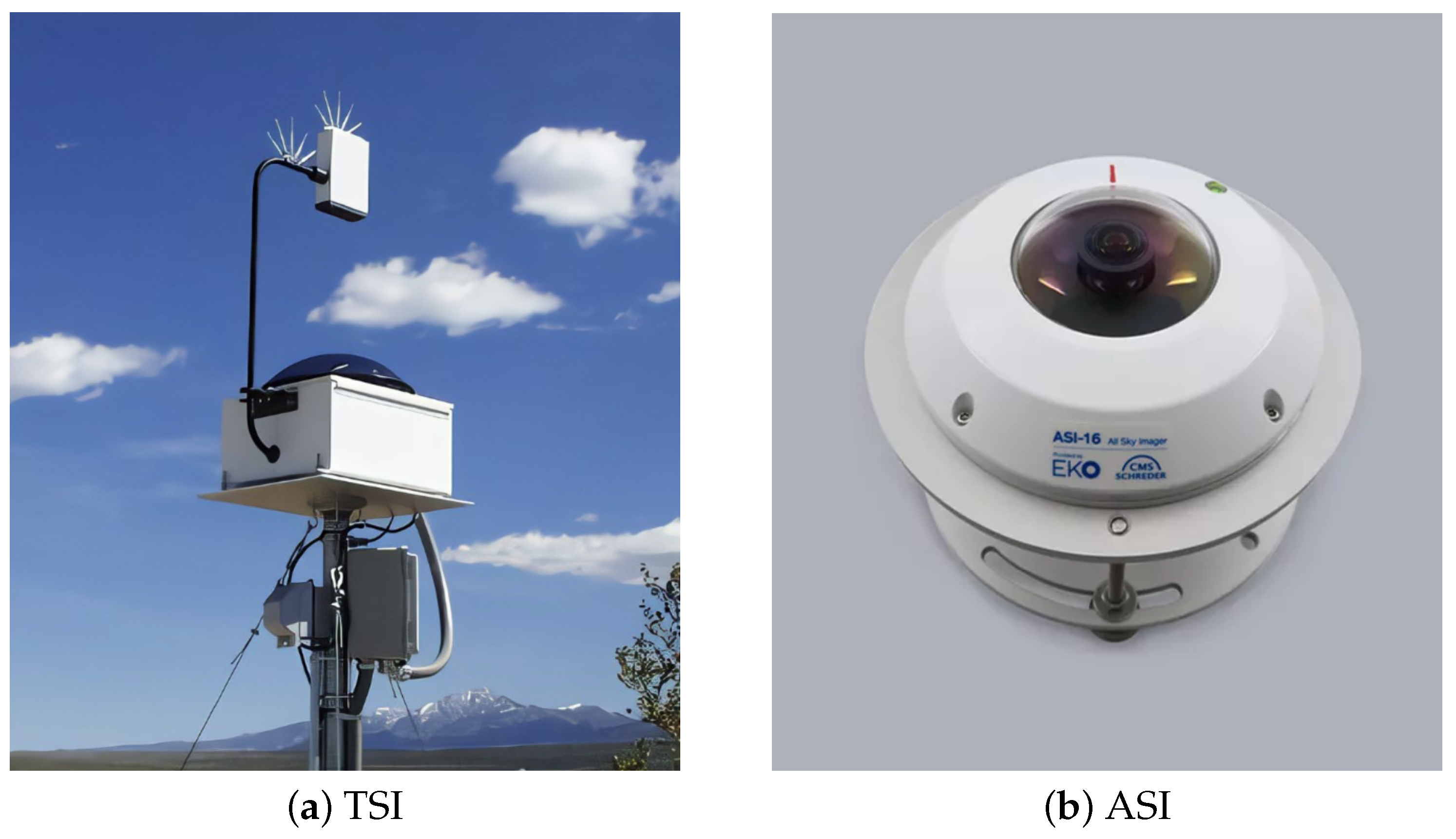
3.1. Dataset Description

The experiments in this paper were conducted on the TJNU ground-based cloud dataset (GCD) [4]. This dataset was collected during 2019 and 2020 in nine Chinese provinces, including Liaoning, Hebei, Tianjin, Shandong, Gansu, Sichuan, Jiangsu, Anhui, and Hainan. A total of 19,000 ground-based images of clouds are contained in the dataset. According to the criteria established by the World Meteorological Organization (WMO)’s international cloud classification system (https://cloudatlas.wmo.int/, accessed on 26 September 2022) and the similarity in visual appearance, seven types of sky conditions can be distinguished. It is remarkable that cloud images whose cloudiness is less than 10% are considered as clear sky. These images are captured using camera sensors and saved with 512 × 512 pixel resolution. Figure 5 shows a few example images included in this data set. Ground-based cloud researchers and meteorologists collaborate to annotate all cloud images. We randomly select 70% samples from each class to form the training set, and the remaining 30% samples are used for testing. The training and test sets do not overlap.

Table 1. Details of GCD dataset.

Cloud Type		Number of Samples			Descriptions
ID	Name	Total	Training	Test
C1	Cumulus	1525	1068	457	Puffy clouds with sharp outlines, flat bottom and raised top, white or light-gray
C2	Altocumulus and Cirrocumulus	1475	1033	442	Patch, sheet or layer of clouds, mosaic-like, white or gray
C3	Cirrus and Cirrostratus	1906	1335	571	Thin clouds, with fibrous (hair-like) appearance, whitish
C4	Clear Sky	3739	2618	1121	Very few or no clouds, blue
C5	Stratocumulus, Stratus and Altostratus	3636	2546	1090	Cloud sheet or layer of striated or uniform appearance, cause fog or fine precipitation, gray or whitish
C6	Cumulonimbus and Nimbostratus	5764	4035	1729	Dark, thick clouds, mostly overcast, cause falling rain or snow, gray
C7	Mixed Clouds	955	669	286	Two or more types of clouds

presents the details of GCD dataset.

3.2. Evaluation Metrics

In order to analyze the classification results of ground-based images quantitatively, we use several widely used evaluation methods, including confusion matrix, overall accuracy, average accuracy, and Kappa coefficient [55]. Confusion matrix, also known as error matrix, forms the basis for analyzing other metrics, such as overall accuracy and Kappa coefficient. Assuming M is the confusion matrix, then its element $m_{ij}$ represents the count of cloud images with real label as i and predicted label as j.

Overall accuracy, or OA, is the ratio of correctly classified images divided by all test images, and it represents the evaluation of the classification results on a global scale. It can be calculated as

$$\begin{array}{c}OA={\displaystyle \sum _{i=1}^c}{m}_{ii}/N\hfill \end{array}$$

(4)

where c is number of cloud types, $m_{ii}$ stands for the diagonal element of M, and $N={\displaystyle \sum _{i=1}^c}{\displaystyle \sum _{j=1}^c}{m}_{ij}$ is the total number of samples that are tested. Average accuracy (AA) is a measure of accuracy averaged over each class.

The Kappa coefficient [56] is calculated using multiple discrete analysis, which incorporates all elements of the confusion matrix. It is generally considered as a more objective measure. The Kappa coefficient can be expressed as follows:

$$\begin{array}{c}\kappa =\frac{N{\displaystyle \sum _{i=1}^c}{m}_{ii}-{\displaystyle \sum _i^c}\left(m_{i+}{m}_{+i}\right)}{N^2-{\displaystyle \sum _i^c}\left(m_{i+}{m}_{+i}\right)}\hfill \end{array}$$

(5)

where $m_{i+}$ denotes the sum of the confusion matrix’s elements in row i and $m_{+i}$ represents that in column i. A higher Kappa coefficient indicates better classification performance.

To evaluate the classification performance of each cloud category, we also use the following measure metrics: precision, recall and F1-score. They are computed by adopting True Positives (TP), False Positives (FP), True Negatives (TN) and False Negatives (FN). The calculations are as follows:

$$\begin{array}{c}precision=\frac{TP}{TP+FP}\hfill \end{array}$$

(6)

$$\begin{array}{c}recall=\frac{TP}{TP+FN}\hfill \end{array}$$

(7)

The F1-score takes both accuracy and precision into account, and can be defined as the harmonic average of them [57]:

$$\begin{array}{c}\frac{1}{F1}=\frac{1}{2}(\frac{1}{precision}+\frac{1}{recall}).\hfill \end{array}$$

(8)

Thus, the F1-score can be computed as

$$\begin{array}{c}F1=2\times \frac{precision\times recall}{precision+recall}=\frac{2\times TP}{2\times TP+FP+FN}.\hfill \end{array}$$

(9)

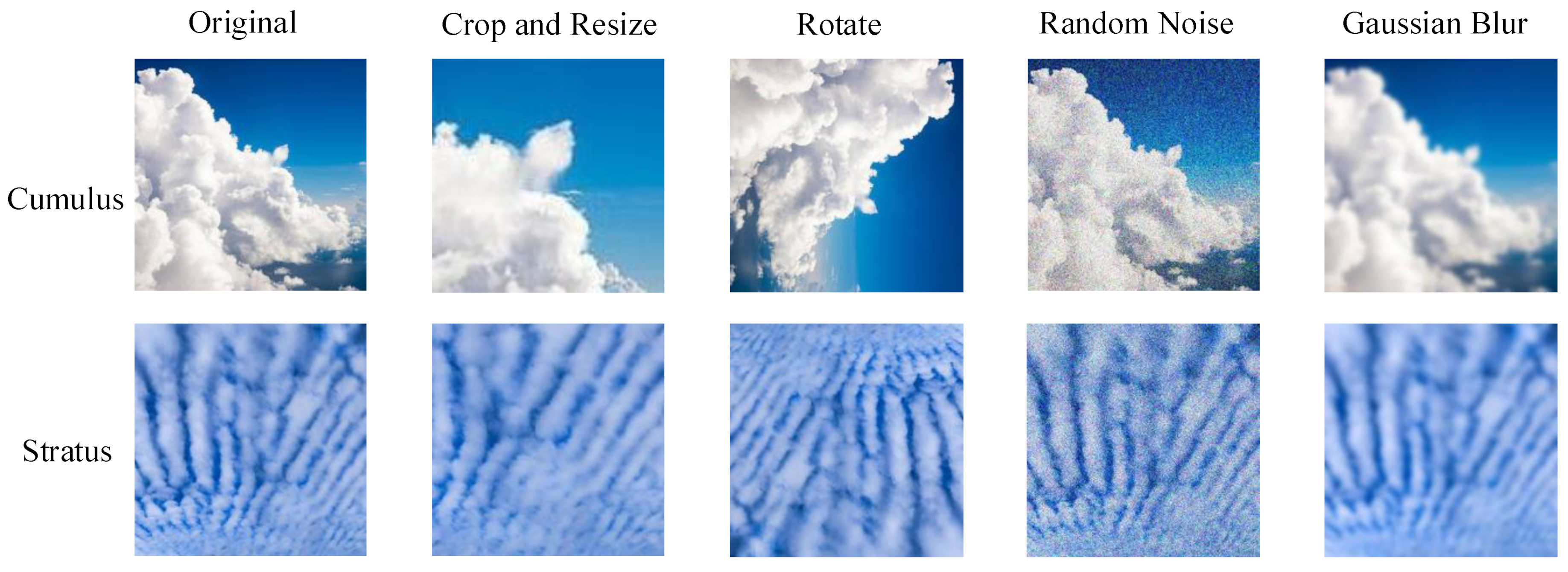
3.3. Experimental Settings

The proposed CSSL method is trained and tested using the PyTorch framework. All experiments were performed on a computer with two ten-core 2.4 GHz Intel Xeon Silver 4210R CPUs, NVIDIA GeForce GTX 3090 GPU and 128 GB memory. In the pre-training procedure, the widely used stochastic gradient descent (SGD) optimizer is applied and the InfoNCE loss mentioned above is utilized as a loss function. We set the learning rate to 0.03 and weight decay to 1 × 10${}^{-4}$. The batch size and epoch number are set to 64 and 200, respectively. Following [49], the feature dimension of projection head is 128, and the max number of negative samples stored in the memory bank is set to be 4096. The temperature parameter in Equation (1) is set as 0.5, and the momentum coefficient in Equation (3) is 0.999.

In the fine-tuning procedure, we utilize the cross-entropy loss as loss function. It is set to 0.01 and 1 × 10${}^{-4}$ for the learning rate and weight decay. The batch size and epoch number are set to 16 and 200, respectively.

3.4. Experimental Results

3.4.1. Classification Performance

Table 2. Performance evaluation of categories in the GCD dataset with the proposed CSSL method.

Category	Precision	Recall	F1-Score
C1	0.9015	0.9212	0.9113
C2	0.8060	0.9118	0.8556
C3	0.8891	0.7863	0.8346
C4	0.9742	0.9777	0.9760
C5	0.7246	0.7459	0.7351
C6	0.8359	0.8398	0.8379
C7	0.7750	0.6503	0.7072

shows the performance assessment of the proposed CSSL method using distinct assessment matrices for each category. As shown in this table, cloud type C4 (clear sky) has excellent classification performance, with precision of 0.9742, recall of 0.9777, and F1-score of 0.9760. C5 (stratocumulus, stratus and altostratus) and C7 (mixed clouds) perform comparatively poorly, with F1-score of 0.7351 and 0.7072, respectively. The remaining cloud types have F1-scores varying from 0.8346 to 0.9113.

Figure 6 shows the confusion matrix of prediction results with the GCD test data set. We can see that only 25 images (2.2%) of cloud type C4 are misclassified, and 36 images (7.9%) are given wrong labels for cloud type C1. Meanwhile, we notice that 219 images of C5 are misclassified to C6, and 225 images of C6 are misclassified to C5, showing a notable confusion between C5 and C6. It is because the cloud types C4 and C1 are clear sky and cumulus, respectively, which possess low diversity; while C5 (stratocumulus, stratus and altostratus) and C6 (cumulonimbus and nimbostratus) have great similarity, which are relatively difficult to distinguish. Further, Figure 7 gives some examples of misclassified images on the GCD dataset, where the ground truth is represented by yellow labels, and predicted cloud categories are indicated by red labels. The interclass misclassification may be brought about by two reasons. The first one is that illumination and viewpoint changes may affect the prediction of cloud categories. For example, the image in the middle of the first row belongs to C2, but it is misjudged as C6, since the illumination makes the cloud turn dark black and it is similar to C6. Second, because the GCD dataset was collected over a period of one year across ten provinces in China, it is highly diverse. Some images are rather difficult to judge, even by experienced experts. Therefore, it is sometimes intractable to make accurate predictions.

3.4.2. Visualization of Features

To visualize the features captured by different layers of the proposed deep model, we show the feature maps of different convolution layers in Figure 8. The fist column contains input cloud images, and it is followed by feature maps in different convolution modules; for instance, Conv1-4 represents the feature map of channel number 4 in the first convolution module. As can be seen from this figure, the shallow layers tend to capture low-level texture information and the shape of clouds is roughly outlined, while the deep layers reflect more abstract high-level semantic features.

3.4.3. Comparison with Other Methods

To verify the effectiveness of our proposed CSSL method, we compare it with several state-of-the-art classification algorithms for ground-based images, including BOMS [29], CloudNet [41], VGG-19 [58], and ResNet-50 [52]. Among these methods, the latter four are deep learning-based. The results are listed in

Table 3. Comparisons with other methods.

Method	OA(%)	AA(%)	Kappa
BOMS [29]	61.76	52.91	0.5092
CloudNet [41]	75.58	69.33	0.6930
VGG-19 [58]	75.32	69.44	0.6921
ResNet-50 [52]	81.00	76.59	0.7637
CSSL	84.62	83.33	0.8093

, where the overall accuracy (OA), average accuracy (AA), and Kappa coefficient are reported. Several conclusions can be made from the table. First, the classification accuracy obtained by BOMs method is relatively low, and the OA is 61.76%. Second, CloudNet and VGG-19 achieve similar classification accuracy, with the OA around 75%. Third, with a deeper architecture, ResNet-50 gets an improvement of over 5% in term of OA compared with CloudNet and VGG-19. Fourth, the CSSL method achieves the best classification results among these approaches, obtaining an OA of 84.62%, an AA of 83.33%, and a Kappa coefficient of 0.8093. The reason behind the superiority of CSSL over ResNet-50 is that, with a self-supervised pre-training procedure, the deep model is assigned a more appropriate set of initial weights. It is worth mentioning that, the training of deep models takes longer than that of the BOMS method, which is a common deficiency of deep models.

For intuitively evaluating CSSL, Figure 9 illustrates the final features of different deep models using t-distributed stochastic neighbor embedding (t-SNE) [59], where the feature visualizations of CloudNet, VGG-19, ResNet-50, and CSSL are shown in Figure 9a–d, respectively. It can be seen that the same color dots in Figure 9d are more closely spaced.

4. Analysis and Discussion

4.1. Effect of the Temperature Parameter

In the loss function, there is an adjustable temperature parameter $\tau$, which has a range of −1 to 1. It plays the role of scaling the input and increasing the range of cosine similarity [60]. The classification results can be affected by a suitable adjustment of the temperature parameter $\tau$. In the experiment, the momentum coefficient is set to 0.999.

Table 4. The OA with different temperature parameter.

$\mathit{\tau }$	0.01	0.05	0.1	0.5	0.8	1.0
OA(%)	82.02	82.53	83.27	84.62	83.58	82.25

shows the results of OA when $\tau$ is set to various values. It has been found that when $\tau$ is 0.5, the most accurate classification is provided.

4.2. Effect of the Momentum Coefficient

In this experiment, we have set the temperature parameter to 0.5.

Table 5. The OA with a different momentum coefficient.

m	0.8	0.9	0.99	0.999	0.9999
OA(%)	80.78	81.34	83.16	84.62	83.97

shows the accuracy of classification with various momentum coefficients, which are used during pre-training as in Equation (3). It behaves decently when m varies between 0.99 and 0.999, indicating the benefit of a slowly progressing auxiliary encoder (i.e., one with a large momentum) [49]. The accuracy has decreased significantly when the value of m is too low (for example, 0.9).

5. Conclusions

In this paper, we propose a classification method of ground-based cloud images based on contrastive self-supervised learning (CSSL). Specifically, data augmentation is applied to the input data at first. Then, contrastive self-supervised learning is used to pre-train the deep model and learn the feature representation of ground-based cloud images, which uses a momentum update strategy. Afterwards, a supervised fine-tuning procedure is adopted to fit the classification mission. Experimental results on the GCD dataset have shown the effectiveness of the proposed CSSL method.

In future work, we will study the case when the labeled samples are extremely insufficient to see how much benefit CSSL can bring. Additionally, the deformable convolution net is considered to be applied as the base encoder in our model, which may be more capable of capturing the rich diversity of cloud shapes. We will further study the CSSL method combined with graph neural networks (GNN) to further improve classification performance of ground-based cloud images.

References

1. Gorodetskaya, I.V.; Kneifel, S.; Maahn, M.; Van Tricht, K.; Thiery, W.; Schween, J.; Mangold, A.; Crewell, S.; Van Lipzig, N. Cloud and precipitation properties from ground-based remote-sensing instruments in East Antarctica. Cryosphere 2015, 9, 285–304. [Google Scholar] [CrossRef] [Green Version]
2. Goren, T.; Rosenfeld, D.; Sourdeval, O.; Quaas, J. Satellite observations of precipitating marine stratocumulus show greater cloud fraction for decoupled clouds in comparison to coupled clouds. Geophys. Res. Lett. 2018, 45, 5126–5134. [Google Scholar] [CrossRef] [PubMed]
3. Zheng, Y.; Rosenfeld, D.; Zhu, Y.; Li, Z. Satellite-based estimation of cloud top radiative cooling rate for marine stratocumulus. Geophys. Res. Lett. 2019, 46, 4485–4494. [Google Scholar] [CrossRef]
4. Liu, S.; Duan, L.; Zhang, Z.; Cao, X.; Durrani, T.S. Ground-Based Remote Sensing Cloud Classification via Context Graph Attention Network. IEEE Trans. Geosci. Remote Sens. 2022, 60, 5602711. [Google Scholar] [CrossRef]
5. Norris, J.R.; Allen, R.J.; Evan, A.T.; Zelinka, M.D.; O’Dell, C.W.; Klein, S.A. Evidence for climate change in the satellite cloud record. Nature 2016, 536, 72–75. [Google Scholar] [CrossRef] [Green Version]
6. Zhong, B.; Chen, W.; Wu, S.; Hu, L.; Luo, X.; Liu, Q. A cloud detection method based on relationship between objects of cloud and cloud-shadow for Chinese moderate to high resolution satellite imagery. IEEE J. Sel. Top. Appl. Earth Obs. Remote Sens. 2017, 10, 4898–4908. [Google Scholar] [CrossRef]
7. Young, A.H.; Knapp, K.R.; Inamdar, A.; Hankins, W.; Rossow, W.B. The international satellite cloud climatology project H-Series climate data record product. Earth Syst. Sci. Data 2018, 10, 583–593. [Google Scholar] [CrossRef] [Green Version]
8. Calbó, J.; Sabburg, J. Feature extraction from whole-sky ground-based images for cloud-type recognition. J. Atmos. Ocean. Technol. 2008, 25, 3–14. [Google Scholar] [CrossRef] [Green Version]
9. Nouri, B.; Wilbert, S.; Segura, L.; Kuhn, P.; Hanrieder, N.; Kazantzidis, A.; Schmidt, T.; Zarzalejo, L.; Blanc, P.; Pitz-Paal, R. Determination of cloud transmittance for all sky imager based solar nowcasting. Sol. Energy 2019, 181, 251–263. [Google Scholar] [CrossRef] [Green Version]
10. Liu, S.; Li, M.; Zhang, Z.; Cao, X.; Durrani, T.S. Ground-Based Cloud Classification Using Task-Based Graph Convolutional Network. Geophys. Res. Lett. 2020, 47. [Google Scholar] [CrossRef]
11. Dev, S.; Wen, B.; Lee, Y.H.; Winkler, S. Ground-based image analysis: A tutorial on machine-learning techniques and applications. IEEE Geosci. Remote Sens. Mag. 2016, 4, 79–93. [Google Scholar] [CrossRef]
12. Chow, C.W.; Urquhart, B.; Lave, M.; Dominguez, A.; Kleissl, J.; Shields, J.; Washom, B. Intra-hour forecasting with a total sky imager at the UC San Diego solar energy testbed. Sol. Energy 2011, 85, 2881–2893. [Google Scholar] [CrossRef] [Green Version]
13. Feister, U.; Shields, J. Cloud and radiance measurements with the VIS/NIR daylight whole sky imager at Lindenberg (Germany). Meteorol. Z. 2005, 14, 627–639. [Google Scholar] [CrossRef]
14. Urquhart, B.; Kurtz, B.; Dahlin, E.; Ghonima, M.; Shields, J.; Kleissl, J. Development of a sky imaging system for short-term solar power forecasting. Atmos. Meas. Tech. 2015, 8, 875–890. [Google Scholar] [CrossRef] [Green Version]
15. Cazorla, A.; Olmo, F.; Alados-Arboledas, L. Development of a sky imager for cloud cover assessment. J. Opt. Soc. Amer. A, Opt. Image Sci. 2008, 25, 29–39. [Google Scholar] [CrossRef]
16. Nouri, B.; Kuhn, P.; Wilbert, S.; Hanrieder, N.; Prahl, C.; Zarzalejo, L.; Kazantzidis, A.; Blanc, P.; Pitz-Paal, R. Cloud height and tracking accuracy of three all sky imager systems for individual clouds. Sol. Energy 2019, 177, 213–228. [Google Scholar] [CrossRef] [Green Version]
17. Ye, L.; Cao, Z.; Xiao, Y. DeepCloud: Ground-based cloud image categorization using deep convolutional features. IEEE Trans. Geosci. Remote Sens. 2017, 55, 5729–5740. [Google Scholar] [CrossRef]
18. Huertas-Tato, J.; Rodríguez-Benítez, F.; Arbizu-Barrena, C.; Aler-Mur, R.; Galvan-Leon, I.; Pozo-Vázquez, D. Automatic cloud-type classification based on the combined use of a sky camera and a ceilometer. J. Geophys. Res. Atmos. 2017, 122, 11045–11061. [Google Scholar] [CrossRef] [Green Version]
19. Li, X.; Qiu, B.; Cao, G.; Wu, C.; Zhang, L. A Novel Method for Ground-Based Cloud Image Classification Using Transformer. Remote Sens. 2022, 14, 3978. [Google Scholar] [CrossRef]
20. Buch Jr, K.A.; Sun, C.H. Cloud classification using whole-sky imager data. In Proceedings of the 9th Symposium on Meteorological Observations and Instrumentation, Charlotte, NC, USA, 27–31 May 1995; pp. 35–39. [Google Scholar]
21. Singh, M.; Glennen, M. Automated ground-based cloud recognition. Pattern Anal. Appl. 2005, 8, 258–271. [Google Scholar] [CrossRef]
22. Heinle, A.; Macke, A.; Srivastav, A. Automatic cloud classification of whole sky images. Atmos. Meas. Tech. 2010, 3, 557–567. [Google Scholar] [CrossRef] [Green Version]
23. Liu, L.; Sun, X.; Chen, F.; Zhao, S.; Gao, T. Cloud classification based on structure features of infrared images. J. Atmos. Ocean. Technol. 2011, 28, 410–417. [Google Scholar] [CrossRef]
24. Isosalo, A.; Turtinen, M.; Pietikäinen, M.; Isosalo, A.; Turtinen, M.; Pietikäinen, M. Cloud characterization using local texture information. In Proceedings of the 2007 Finnish Signal Processing Symposium (FINSIG 2007), Oulu, Finland, 30 August 2007. [Google Scholar]
25. Liu, S.; Wang, C.; Xiao, B.; Zhang, Z.; Shao, Y. Salient local binary pattern for ground-based cloud classification. Acta Meteorol. Sin. 2013, 27, 211–220. [Google Scholar] [CrossRef]
26. Wang, Y.; Shi, C.; Wang, C.; Xiao, B. Ground-based cloud classification by learning stable local binary patterns. Atmos. Res. 2018, 207, 74–89. [Google Scholar] [CrossRef]
27. Oikonomou, S.; Kazantzidis, A.; Economou, G.; Fotopoulos, S. A local binary pattern classification approach for cloud types derived from all-sky imagers. Int. J. Remote Sens. 2019, 40, 2667–2682. [Google Scholar] [CrossRef]
28. Zhuo, W.; Cao, Z.; Xiao, Y. Cloud classification of ground-based images using texture–structure features. J. Atmos. Ocean. Technol. 2014, 31, 79–92. [Google Scholar] [CrossRef]
29. Li, Q.; Zhang, Z.; Lu, W.; Yang, J.; Ma, Y.; Yao, W. From pixels to patches: A cloud classification method based on a bag of micro-structures. Atmos. Meas. Tech. 2016, 9, 753–764. [Google Scholar] [CrossRef] [Green Version]
30. LeCun, Y.; Bengio, Y.; Hinton, G. Deep learning. Nature 2015, 521, 436–444. [Google Scholar] [CrossRef]
31. Schmidhuber, J. Deep learning in neural networks: An overview. Neural Netw. 2015, 61, 85–117. [Google Scholar] [CrossRef] [Green Version]
32. Liu, W.; Wang, Z.; Liu, X.; Zeng, N.; Liu, Y.; Alsaadi, F.E. A survey of deep neural network architectures and their applications. Neurocomputing 2017, 234, 11–26. [Google Scholar] [CrossRef]
33. Khanafer, M.; Shirmohammadi, S. Applied AI in instrumentation and measurement: The deep learning revolution. IEEE Instrum. Meas. Mag. 2020, 23, 10–17. [Google Scholar] [CrossRef]
34. Wen, G.; Gao, Z.; Cai, Q.; Wang, Y.; Mei, S. A novel method based on deep convolutional neural networks for wafer semiconductor surface defect inspection. IEEE Trans. Instrum. Meas. 2020, 69, 9668–9680. [Google Scholar] [CrossRef]
35. Lin, Y.H.; Chang, L. An Unsupervised Noisy Sample Detection Method for Deep Learning-Based Health Status Prediction. IEEE Trans. Instrum. Meas. 2022, 71, 2502211. [Google Scholar] [CrossRef]
36. Bengio, Y.; Courville, A.; Vincent, P. Representation learning: A review and new perspectives. IEEE Trans. Pattern Anal. Mach. Intell. 2013, 35, 1798–1828. [Google Scholar] [CrossRef] [Green Version]
37. Reichstein, M.; Camps-Valls, G.; Stevens, B.; Jung, M.; Denzler, J.; Carvalhais, N. Deep learning and process understanding for data-driven Earth system science. Nature 2019, 566, 195–204. [Google Scholar] [CrossRef]
38. Yuan, Q.; Shen, H.; Li, T.; Li, Z.; Li, S.; Jiang, Y.; Xu, H.; Tan, W.; Yang, Q.; Wang, J.; et al. Deep learning in environmental remote sensing: Achievements and challenges. Remote Sens. Environ. 2020, 241, 111716. [Google Scholar] [CrossRef]
39. Ye, L.; Cao, Z.; Xiao, Y.; Li, W. Ground-based cloud image categorization using deep convolutional visual features. In Proceedings of the 2015 IEEE International Conference on Image Processing (ICIP), Quebec City, QC, Canada, 27–30 September 2015; pp. 4808–4812. [Google Scholar]
40. Shi, C.; Wang, C.; Wang, Y.; Xiao, B. Deep convolutional activations-based features for ground-based cloud classification. IEEE Geosci. Remote Sens. Lett. 2017, 14, 816–820. [Google Scholar] [CrossRef]
41. Zhang, J.; Liu, P.; Zhang, F.; Song, Q. CloudNet: Ground-based cloud classification with deep convolutional neural network. Geophys. Res. Lett. 2018, 45, 8665–8672. [Google Scholar] [CrossRef]
42. Wang, M.; Zhou, S.; Yang, Z.; Liu, Z. CloudA: A Ground-Based Cloud Classification Method with a Convolutional Neural Network. J. Atmos. Ocean. Technol. 2020, 37, 1661–1668. [Google Scholar] [CrossRef]
43. Liu, S.; Duan, L.; Zhang, Z.; Cao, X.; Durrani, T.S. Multimodal ground-based remote sensing cloud classification via learning heterogeneous deep features. IEEE Trans. Geosci. Remote Sens. 2020, 58, 7790–7800. [Google Scholar] [CrossRef]
44. Liu, S.; Li, M.; Zhang, Z.; Xiao, B.; Cao, X. Multimodal ground-based cloud classification using joint fusion convolutional neural network. Remote Sens. 2018, 10, 822. [Google Scholar] [CrossRef] [Green Version]
45. Liu, S.; Li, M.; Zhang, Z.; Xiao, B.; Durrani, T.S. Multi-evidence and multi-modal fusion network for ground-based cloud recognition. Remote Sens. 2020, 12, 464. [Google Scholar] [CrossRef] [Green Version]
46. Jing, L.; Tian, Y. Self-supervised visual feature learning with deep neural networks: A survey. IEEE Trans. Pattern Anal. Mach. Intell. 2021, 43, 4037–4058. [Google Scholar] [CrossRef]
47. Liu, X.; Zhang, F.; Hou, Z.; Mian, L.; Wang, Z.; Zhang, J.; Tang, J. Self-supervised learning: Generative or contrastive. IEEE Trans. Knowl. Data Eng. 2021, in press. [Google Scholar] [CrossRef]
48. Chen, T.; Kornblith, S.; Norouzi, M.; Hinton, G. A simple framework for contrastive learning of visual representations. In Proceedings of the the 37th International Conference on Machine Learning (ICML 2020), Virtual, 13–18 July 2020; pp. 1597–1607. [Google Scholar]
49. He, K.; Fan, H.; Wu, Y.; Xie, S.; Girshick, R. Momentum contrast for unsupervised visual representation learning. In Proceedings of the 2020 IEEE/CVF Conference on Computer Vision and Pattern Recognition (CVPR 2020), Seattle, WA, USA, 13–19 June 2020; pp. 9729–9738. [Google Scholar]
50. Caron, M.; Misra, I.; Mairal, J.; Goyal, P.; Bojanowski, P.; Joulin, A. Unsupervised learning of visual features by contrasting cluster assignments. In Proceedings of the Advances in Neural Information Processing Systems (NeurIPS 2020), Virtual, 6–12 December 2020. [Google Scholar]
51. Grill, J.B.; Strub, F.; Altché, F.; Tallec, C.; Richemond, P.H.; Buchatskaya, E.; Doersch, C.; Pires, B.A.; Guo, Z.D.; Azar, M.G.; et al. Bootstrap your own latent: A new approach to self-supervised learning. In Proceedings of the Advances in Neural Information Processing Systems (NeurIPS 2020), Virtual, 6–12 December 2020. [Google Scholar]
52. He, K.; Zhang, X.; Ren, S.; Sun, J. Deep residual learning for image recognition. In Proceedings of the 2016 IEEE/CVF Conference on Computer Vision and Pattern Recognition (CVPR 2016), Las Vegas, NV, USA, 27–30 June 2016; pp. 770–778. [Google Scholar]
53. Oord, A.v.d.; Li, Y.; Vinyals, O. Representation learning with contrastive predictive coding. arXiv 2018, arXiv:1807.03748. [Google Scholar]
54. Zhang, L.; Zhang, S.; Zou, B.; Dong, H. Unsupervised deep representation learning and few-shot classification of PolSAR images. IEEE Trans. Geosci. Remote Sens. 2022, 60, 5100316. [Google Scholar] [CrossRef]
55. Lv, Q.; Dou, Y.; Xu, J.; Niu, X.; Xia, F. Hyperspectral image classification via local receptive fields based random weights networks. In Proceedings of the 2015 International Conference on Natural Computation (ICNC), Zhangjiajie, China, 15–17 August 2015; pp. 971–976. [Google Scholar]
56. Thompson, W.D.; Walter, S.D. A reappraisal of the kappa coefficient. J. Clin. Epidemiol. 1988, 41, 949–958. [Google Scholar] [CrossRef]
57. Powers, D.M.W. Evaluation: From precision, recall and F-measure to ROC, informedness, markedness and correlation. J. Mach. Learn. Technol. 2011, 2, 37–63. [Google Scholar]
58. Simonyan, K.; Zisserman, A. Very deep convolutional networks for large-scale image recognition. arXiv 2014, arXiv:1409.1556. [Google Scholar]
59. Van der Maaten, L.; Hinton, G. Visualizing data using t-SNE. J. Mach. Learn. Res. 2008, 9, 2579–2605. [Google Scholar]
60. Hou, S.; Shi, H.; Cao, X.; Zhang, X.; Jiao, L. Hyperspectral Imagery Classification Based on Contrastive Learning. IEEE Trans. Geosci. Remote Sens. 2022, 60, 5521213. [Google Scholar] [CrossRef]
Figure 1. Examples of Total Sky Imager (TSI) (source of picture: https://gml.noaa.gov/grad/surfrad/tsipics.html, accessed on 30 October 2022) and All Sky Imager (ASI) (source of picture: https://www.eko-instruments.com, accessed on 30 October 2022). (a) The TSI is composed of a web camera suspended over a convex mirror. (b) The ASI-16 All Sky Imager utilizes a 5MP camera and fish-eye lens with an anti-reflective coated quartz dome.
Remotesensing 14 05821 g001
Figure 2. Schematic diagram of the proposed method.
Remotesensing 14 05821 g002
Figure 3. Examples of data augmentation.
Remotesensing 14 05821 g003
Figure 4. Pre-training of DNN using contrastive SSL.
Remotesensing 14 05821 g004
Figure 5. Example images from 7-class GCD dataset: (a) Cumulus, (b) Altocumulus and Cirrocumulus, (c) Cirrus and Cirrostratus, (d) Clear Sky, (e) Stratocumulus, Stratus and Altostratus, (f) Cumulonimbus and Nimbostratus, (g) Mixed Clouds.
Remotesensing 14 05821 g005
Figure 6. Confusion matrix of the proposed CSSL method.
Remotesensing 14 05821 g006
Figure 7. Misclassified images on the GCD dataset. Ground truth is represented by yellow labels, and predicted cloud types are indicated by red labels.
Remotesensing 14 05821 g007
Figure 8. Visualization of feature maps from different convolution layers.
Remotesensing 14 05821 g008
Figure 9. Visualizations of features based on t-SNE [59], in which each dot represents the final feature of the ground-based cloud image, and the types of clouds are indicated by their colors. Feature visualizations of (a) CloudNet, (b) VGG-19, (c) ResNet-50, and (d) CSSL.
Remotesensing 14 05821 g009aRemotesensing 14 05821 g009b