On the Co-Selection of Vision Transformer Features and Images for Very High-Resolution Image Scene Classification

Abstract

Recent developments in remote sensing technology have allowed us to observe the Earth with very high-resolution (VHR) images. VHR imagery scene classification is a challenging problem in the field of remote sensing. Vision transformer (ViT) models have achieved breakthrough results in image recognition tasks. However, transformer–encoder layers encode different levels of features, where the latest layer represents semantic information, in contrast to the earliest layers, which contain more detailed data but ignore the semantic information of an image scene. In this paper, a new deep framework is proposed for VHR scene understanding by exploring the strengths of ViT features in a simple and effective way. First, pre-trained ViT models are used to extract informative features from the original VHR image scene, where the transformer–encoder layers are used to generate the feature descriptors of the input images. Second, we merged the obtained features as one signal data set. Third, some extracted ViT features do not describe well the image scenes, such as agriculture, meadows, and beaches, which could negatively affect the performance of the classification model. To deal with this challenge, we propose a new algorithm for feature- and image selection. Indeed, this gives us the possibility of eliminating the less important features and images, as well as those that are abnormal; based on the similarity of preserving the whole data set, we selected the most informative features and important images by dropping the irrelevant images that degraded the classification accuracy. The proposed method was tested on three VHR benchmarks. The experimental results demonstrate that the proposed method outperforms other state-of-the-art methods.

1. Introduction

The high-speed development of remote sensing instruments and technologies has provided us with the ability to capture high and very high-resolution (VHR) images. This raises challenging problems concerning appropriate and efficient methods for image scene understanding and classification. The classification of VHR images into the corresponding and adequate classes of the same semantics (according to the image scene) is critical. In the last decade, several methods have been proposed for VHR image scene understanding. The existing scene classification methods are distinguished by three categories, which depend on the pixel-/object-level image representation, in which the VHR image scene classification techniques directly depend on the holistic representation of the image scene as demonstrated in [1]. These kinds of methods represent the VHR image scenes with handcrafted features, which are also called low-level features, such as texture descriptors [2], color histogram (CH) [3], the scale-invariant feature transform (SIFT) [4], and the histogram of the oriented gradient (HOG) [5].

Several works based on low-level features have been developed for VHR image scene classification. Yang and Newsam [6] compared Gabor texture features and SIFT features for the IKONOS remote sensing image classification, and Dos-Santos et al. [2] evaluated the CH descriptor and local binary patterns (LBP) for remote sensing image retrieval and classification [7]. As demonstrated in [6,7,8], image scene classification based on a single kind of low-level feature achieved high accuracy.

Unfortunately, in real applications, one single feature is not able to well represent the entire information of the image scene, so scene information is usually described by a set of descriptors, which better improves the results than singular features [9,10]. Lou et al. [11] combined the Gabor filters, SIFT features, simple radiometric features, Gaussian wavelet features [12], gray level co-occurrence matrix (GLCM), and shape features [13], with the aim to form a global features representation for remote sensing image indexing. Avramovic and Risojevic [14] proposed combining SIFT with GIST features for aerial scene classification. In addition, other approaches were developed to select a subset of low-level features for aerial image classification [15]. Although the combination of low-level features can often improve the results, how to effectively combine different types of features is a challenging problem. Moreover, handcrafted features are not capable of accurately representing the entire content of the image scene, especially when the scene images become more challenging. To alleviate this concern, other techniques have been developed for image scene descriptions based on mid-level features.

Mid-level approaches [16,17,18] often represent the image scene by coding low-level feature descriptors. To describe the entire image scene, they build blocks to construct the global image features, such as the bag of visual words (BOVW) [19], which is the most popular encoding model for remote sensing image scene descriptions [20,21,22,23], and the HOG feature-based models [24].

Approaches based on low-level and mid-level features require a considerable amount of engineering skills and domain expertise for the VHR image scene understanding. To overcome this limit, deep learning-based methods were introduced to classify remote sensing images, which learned features from input data using a general-purpose learning procedure via the deep architecture of neural networks. The main advantage of deep learning methods is the ability to learn more informative and powerful features to describe the input data with several levels of abstraction [25].

Convolutional neural networks (CNNs) and their variants are popular deep learning models that have proven their effectiveness for image scene classifications as demonstrated with ImageNet large-scale visual recognition competition (ILSVRC) [26]. CNNs can learn the image scene by leveraging a hierarchical representation that describes the content of an image. Recently, CNNs have become widely applied in remote sensing image analyses, thus becoming more suitable for scene classification and retrieval from VHR images [25].

Based on the combination of various deep neural networks for VHR image scene interpretations, Zhang et al. [27] introduced a novel framework that achieved specifiable results when applied to the UC Merced data set [28]. The small sizes of remote sensing data sets make it extremely hard to train new a CNN model [29]. However, pre-trained CNN models have achieved acceptable results for VHR remote sensing image scene classification [30]. In this context, Othman et al. [30] leveraged pre-trained CNN models to generate the preliminary representation features from an image scene; they applied a sparse autoencoder that learned the final feature description of the target image. In the same vein, Hu et al. [25] employed pre-trained CNNs for scene classification in two different ways. In the fist way, they used two fully connected layers as final feature descriptors of the target images. In the second step, they applied convolutional layers as initial feature descriptors of the target image scenes with different scale sizes, then they took advantage of popular coding approaches, such as BOVW, to encode the dense convolutional features into a global features descriptor.

In recent years, transformers have revolutionized the field of deep learning. Transformers have achieved extraordinary results in different challenges of natural language processing (NLP) [31,32]. Encouraged by the success of transformer models in the NLP area, there have been important advances in transformers in computer vision tasks. ViT models achieved great results in various challenges of computer vision, such as image classification [33]. As mentioned in [34], deep feature fusion is an efficient technique for understanding remote sensing images. In this study, we explored the use of the vision transformer for VHR image scene classification. We focused on using pre-trained ViT models to extract feature descriptors from VHR images in order to generate global image description vectors for image scene representation. In summary, the contributions of this paper are three-fold:

1.

We explore the performance of the vision transformer method based on the pre-trained ViT model. The transformer–encoder layer is considered a feature descriptor, where a discriminative image scene representation is generated from the transformer–encoder layer.

2.

Second, we present a new approach that consists of selecting the most important features and images and detecting unwanted and noisy images. Indeed, these images can have negative impacts on the accuracy of the final model. By doing so, we obtained a good data set without noise, which allowed us to have good accuracy and, consequently, reduce the learning time.

3.

Another challenging problem in understanding a VHR image scene involves the classification strategy. To this end, we used the support vector machine (SVM) to classify the extracted ViT features corresponding to the selected encoder layers.

The rest of the paper is organized as follows. Section 2 introduces the proposed framework and the processing pipelines to extract the feature descriptor for VHR image scene classification. Firstly, we introduce the pre-trained ViT model to automatically extract features from the VHR images. Second, we present the proposed approach, which consists of selecting the most important features and images. The sub-selection allows for achieving good accuracy and reduces the learning time. Finally, we present the last block of our framework in which we learn a classification model from the data set obtained by the co-selection step. The experimental results from various databases are presented in Section 3. Finally, we conclude the paper in Section 4.

2. Proposed Framework

In this section, we describe the three blocks that are the bases of our VHR Image classification framework.

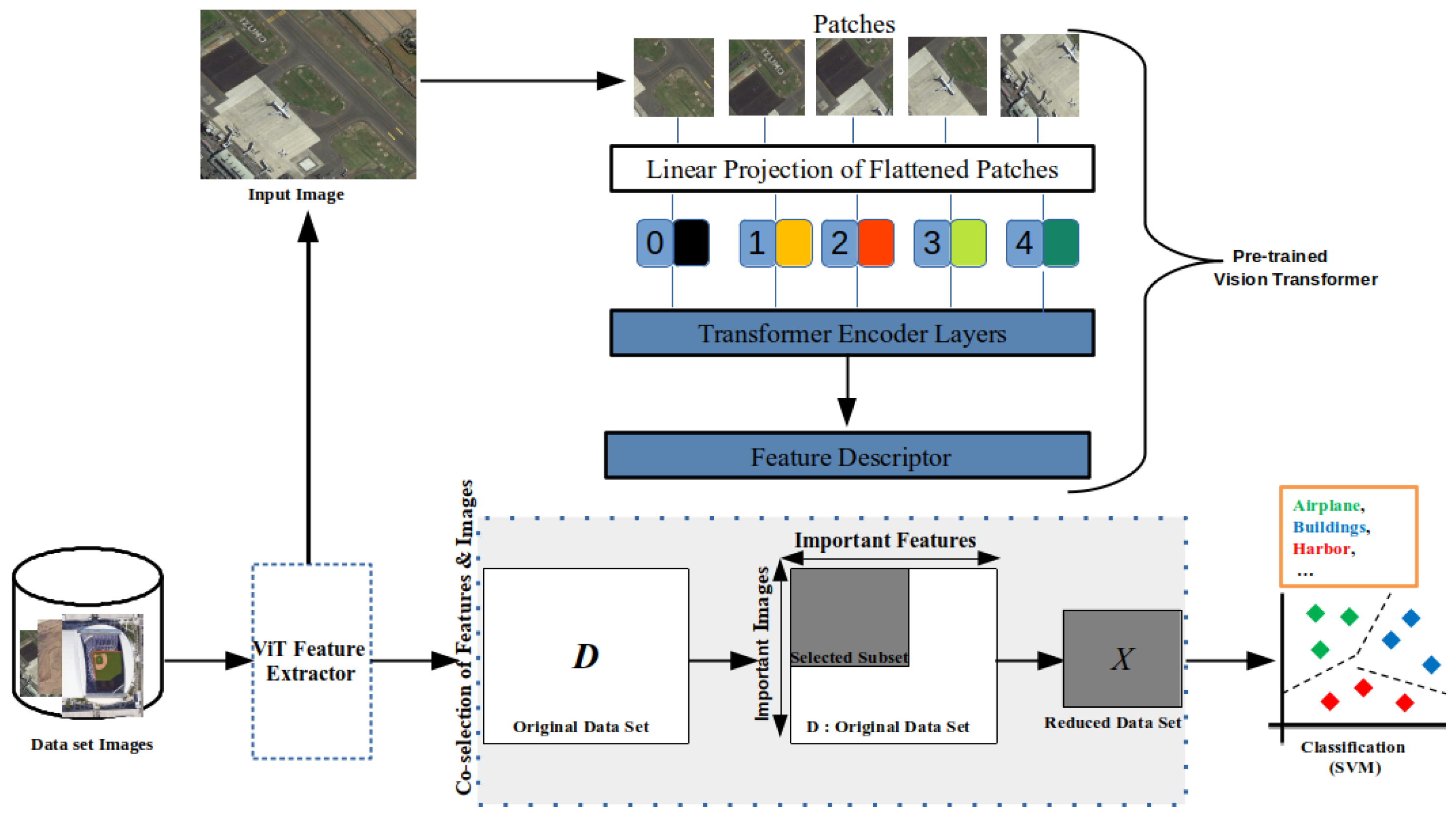
The idea of the framework is to transform the input images with four ViT models and merge the features obtained to obtain a single raw data set containing all features (Figure 1). However, such a data set can have redundant and highly correlated features. Therefore, a feature selection step is required. In addition, some images in VHR data sets may be abnormal, which can degrade the quality of the classifier during the training phase. That is why we propose selecting both features and images in order to have the best data set for the learning step (unlike other frameworks that focus only on feature selection or reduction). Then, we create a classification model on top of the obtained data set.

2.1. ViT Model and Feature Fusion

In order to represent the image scene, we put the VHR images into four different models, i.e., $ViT{8}_b$, $ViT{16}_b$, $ViT{8}_s$, and $ViT{16}_s$, where the transformer–encoder layer is considered a final feature descriptor of the image scene. The four models encode the input image scenes with different dimensions as shown in the following

Table 1. Dimensions of the four ViT models.

	$\mathit{ViT}{8}_b$	$\mathit{ViT}{16}_b$	$\mathit{ViT}{8}_s$	$\mathit{ViT}{16}_s$
Dimension	768	768	384	384

:

Let X be the set of n input images, and ${\mathrm{\Phi }}_m(.)$ the map function that transforms each image ${\mathbf{x}}_i$ to a feature vector ${\mathbf{v}}_i$ according to the model m, such that m is one of the four ViT models, $m\in \{ViT{8}_b,ViT{16}_b,ViT{8}_s,ViT{16}_s\}$.

We denote by ${\mathbf{V}}_m$ the matrix that contains all vectors ${\mathbf{v}}_i$ generated from the images X by the model m:

$${\mathrm{\Phi }}_m(.):\mathbf{X}⟶{\mathbf{V}}_m\in R^{n\times d_m}$$

where $d_m$ is the number of features extracted by model m.

We represent by $\widehat{\mathbf{V}}\in R^{n\times p}$ the concatenation of all features generated by the four models:

$$\widehat{\mathbf{V}}=\bigcup _{m=1}^4{\mathrm{\Phi }}_m\left(\mathbf{X}\right)$$

(1)

where

$$p=\sum _{m=1}^4{d}_m$$

is the number of all features.

2.2. Co-Selection of Features and Images

We select the most important ViT features based on the similarity-preservation of the input images; we also select the most important images and drop the irrelevant ones. In fact, these anomalous images can degrade the quality of the classifier. Unlike other approaches that focus only on feature selection or reduction, we select the most important images (instances) and drop anomalous images that can degrade the quality of the classifier. We will describe how we perform this co-selection before describing the different components of our proposed framework.

First, in order to select the most important features, we rely on the similarity preserving technique that consists of finding a projection matrix Q, which transforms the data set $\widehat{\mathbf{V}}$ to a low-dimensional one $\widehat{\mathbf{V}}\mathbf{Q}$ in order to preserve the similarity of $\widehat{\mathbf{V}}$ with $\widehat{\mathbf{V}}$Q by minimizing the difference between the similar structure in the original space and the low-dimensional one:   

$$\underset{\mathbf{Q}}{min}\Vert \widehat{\mathbf{V}}\mathbf{Q}{\mathbf{Q}}^T{\widehat{\mathbf{V}}}^T{-\mathbf{A}\Vert }_F^2+\lambda {\Vert \mathbf{Q}\Vert }_{2,1}$$

(2)

where

• Q is a projection matrix to be estimated. It is of dimension ($p\times h$) where $h<p$ and h denote the sizes of the new feature set.
• A is a binary matrix, which is derived from the label information $\mathbf{Y}=[y_i,\cdots ,y_n]$ as follows:

  $${\mathbf{A}}_{ij}=\left\{\begin{array}{c}1\mathrm{if}{y}_i=y_j\hfill \\ 0\mathrm{if}{y}_i\ne y_j\hfill \end{array}\right.$$

  (3)
• $\lambda$ is a regularization hyperparameter used to control the sparsity of the projection matrix Q.
• ${\Vert .\Vert }_{2,1}$ is the ${\ell }_{2,1}$-norm. If $\mathbf{P}$ is $(n\times m)$ matrix, then its ${\ell }_{2,1}$-norm is defined by:

  $${\Vert \mathbf{P}\Vert }_{2,1}=\sum _{i=1}^m{\Vert {\mathbf{P}}_i\Vert }_2=\sum _{i=1}^m\sqrt{\sum _{j=1}^n{\mathbf{P}}_{ij}^2}$$

  (4)
• ${\Vert .\Vert }_F$ is the Frobenius norm (${\ell }_{2,2}$) defined by:

  $${\Vert \mathbf{P}\Vert }_F=\left(\sum _{i=1}^m{\Vert {\mathbf{P}}_i\Vert }_2^2\right)={\left(\sum _{i=1}^m\left(\sum _{j=1}^n{\mathbf{P}}_{ij}^2\right)\right)}_{}^{1/2}$$

  (5)

However, the above optimization problem is NP-hard and cannot be solved as shown in [35]. This leads to a reformulation of the problem as follows:

$$\underset{\mathbf{Q}}{min}\Vert \widehat{\mathbf{V}}{\mathbf{Q}-\mathbf{K}\Vert }_F^2+\lambda {\Vert \mathbf{Q}\Vert }_{2,1}$$

(6)

where $\mathbf{K}\in R^{n\times h}$ can be obtained by an eigendecomposition of the binary matrix A, such that:

$$\mathbf{A}={\mathbf{KK}}^T$$

Once the projection matrix $\mathbf{Q}$ is fitted, the features can be ranked according to the ${\ell }_{2,1}$-norms of the rows of the matrix $\mathbf{Q}$. In fact, each row in $\mathbf{Q}$ corresponds to a feature importance and a large ${\ell }_{2,1}$-norm of the ith row of $\mathbf{Q}$ indicates that the ith feature of $\widehat{\mathbf{V}}$ is important.

Second, in order to drop the irrelevant images and select the most representative ones for the classification task, we propose modifying the objective function in (6) by adding a residual matrix $\mathbf{R}\in R^{h\times n}$ to weigh the images [36]. We define this matrix by ${\mathbf{Q}}^T{\widehat{\mathbf{V}}}^T-{\mathbf{K}}^T-\mathrm{\Theta }$, where $\mathrm{\Theta }$ is a random matrix, usually assumed to be a multi-dimensional normal distribution [37]. Exploiting the R matrix is a good way to detect and identify anomalies in a data set. Each column of R corresponds to an image and a large norm of $\mathbf{R}(:,i)$ shows a significant deviation of the ith image, which is more likely to be an irrelevant image. Thus, we propose detecting both irrelevant features and images by solving the following problem:

$$\underset{\mathbf{Q},\mathbf{R}}{min}\Vert \widehat{\mathbf{V}}\mathbf{Q}-{\mathbf{R}}^T{-\mathbf{K}\Vert }_F^2+{\lambda \Vert \mathbf{Q}\Vert }_{2,1}+\beta {\Vert \mathbf{R}\Vert }_{2,1}$$

(7)

where:

• $\beta$ is a regularization hyperparameter used to control the sparsity of the residual matrix R.

The first term in Equation (7) exploits the data structure by preserving the pairwise sample similarities of the images. The second and third terms are used to perform feature selection and image selection, respectively.

2.3. Optimization

To solve the problem in Equation (7), we adopt an alternating optimization over Q and R by solving two reduced minimization problems:

Problem 1:

Minimizing Equation (7) by fixing R to find the solution for Q (for the feature selection). To solve this problem, we consider the Lagrangian of Equation (7):

$${\mathcal{L}}_Q=trace({\mathbf{Q}}^T{\widehat{\mathbf{V}}}^T\widehat{\mathbf{V}}\mathbf{Q}-2{\mathbf{Q}}^T{\widehat{\mathbf{V}}}^T({\mathbf{R}}^T+\mathbf{K}))+\lambda {\Vert \mathbf{Q}\Vert }_{2,1}.$$

(8)

Then, we calculate the derivative of ${\mathcal{L}}_Q$ w.r.t Q:

$$\frac{\partial {\mathcal{L}}_W}{\partial \mathbf{Q}}=2{\widehat{\mathbf{V}}}^T\widehat{\mathbf{V}}\mathbf{Q}-2{\widehat{\mathbf{V}}}^T({\mathbf{R}}^T+\mathbf{K})+2\lambda {\mathcal{D}}_Q\mathbf{Q}.$$

(9)

where ${\mathcal{D}}_Q$ is a ($p\times p$) diagonal matrix with the ith element equal to $\frac{1}{{2\Vert \mathbf{Q}(i,:)\Vert }_2}$.

Subsequently, we set the derivative to zero to update Q by the following formula:

$$\mathbf{Q}={({\widehat{\mathbf{V}}}^T\widehat{\mathbf{V}}+\lambda {\mathcal{D}}_Q)}^{-1}{\widehat{\mathbf{V}}}^T({\mathbf{R}}^T+\mathbf{K})$$

(10)

Problem 2: Minimizing Equation (7) by fixing Q to find the solution for R (for image selection). To solve this problem, we consider the Lagrangian of Equation (7):

$${\mathcal{L}}_R=trace({\mathbf{R}}^T\mathbf{R}-2{\mathbf{R}}^T(\widehat{\mathbf{V}}\mathbf{Q}-\mathbf{K}))+\beta {\Vert \mathbf{R}\Vert }_{2,1}.$$

(11)

Then, we calculate the derivative of ${\mathcal{L}}_R$ w.r.t R:

$$\frac{\partial {\mathcal{L}}_R}{\partial \mathbf{R}}=2{\mathbf{R}}^T-2(\widehat{\mathbf{V}}\mathbf{Q}-\mathbf{K})+2\beta {\mathcal{D}}_R{\mathbf{R}}^T.$$

(12)

where ${\mathcal{D}}_R$ is a ($n\times n$) diagonal matrix with the ith element equal to $\frac{1}{2\Vert {\mathbf{R}}^T{(i,:)\Vert }_2}$.

Subsequently, we set the derivative to zero to update R by the following formula:

$$\mathbf{R}={(\widehat{\mathbf{V}}\mathbf{Q}-\mathbf{K})}^T{\left({(\mathbf{I}+\beta {\mathcal{D}}_R)}^{-1}\right)}^T$$

(13)

where I is an ($n\times n$) identity matrix. We summarize all of the above mathematical developments on Algorithm 1.

Algorithm 1 The Proposed Framework

Input: Data set X of n images and the label information $\mathbf{Y}$; the map function ${\mathrm{\Phi }}_m(.)$ of the deep model m; the hyperparameters: $\lambda ,\beta \mathrm{and}h$. Output: the fitted Q and R. 1: Transform the images X by the four ViT models according to Equation (1) to obtain $\widehat{\mathbf{V}}$. 2: Randomly split the data set $(\widehat{\mathbf{V}},\mathbf{Y})$ into train and test sets (${\widehat{\mathbf{V}}}_{\mathrm{train}}$, ${\widehat{\mathbf{V}}}_{\mathrm{test}}$, ${\mathbf{Y}}_{\mathrm{train}}$, ${\mathbf{Y}}_{\mathrm{test}}$). 3: Calculate A according to Equation (3) over ${\mathbf{Y}}_{\mathrm{train}}$. 4: Eigen-decompose A such as $\mathbf{A}={\mathbf{KK}}^T$. 5: Set ${\mathcal{D}}_Q$ and ${\mathcal{D}}_R$ as identity matrices and R to zero-matrix. 6: repeat 7:    Update Q according to Equation (10) over ${\widehat{\mathbf{V}}}_{\mathrm{train}}$. 8:    Update R according to Equation (13) over ${\widehat{\mathbf{V}}}_{\mathrm{train}}$. 9:    Update ${\mathcal{D}}_R$ and ${\mathcal{D}}_Q$. 10: untilConvergence 11: Rank the features according to ${\Vert \mathbf{Q}(j,:)\Vert }_2$ in descending order ($j=1\cdots p$) and the images according to ${\Vert \mathbf{R}(:,i)\Vert }_2$ in ascending order ($i=1\cdots n$). 12: Remove the irrelevant features and images from over ${\widehat{\mathbf{V}}}_{\mathrm{train}}$ and over ${\widehat{\mathbf{V}}}_{\mathrm{test}}$. 13: Learn a classification model by SVM on the new data set (${\widehat{\mathbf{V}}}_{\mathrm{train}\_\mathrm{new}}$, ${\widehat{\mathbf{V}}}_{\mathrm{text}\_\mathrm{new}}$, ${\mathbf{Y}}_{\mathrm{train}\_\mathrm{new}}$, ${\mathbf{Y}}_{\mathrm{text}\_\mathrm{new}}$).

3. Experimental Results and Setup

The proposed method was evaluated on three different–public–very high spatial resolution data sets (UC Merced, AID, and NWPU-RESISC45). First, the data sets used are described in the flowing subsection, where we also analyze the parameters of the proposed approach. The results of the scene classification for each data set are then discussed.

3.1. Data Sets

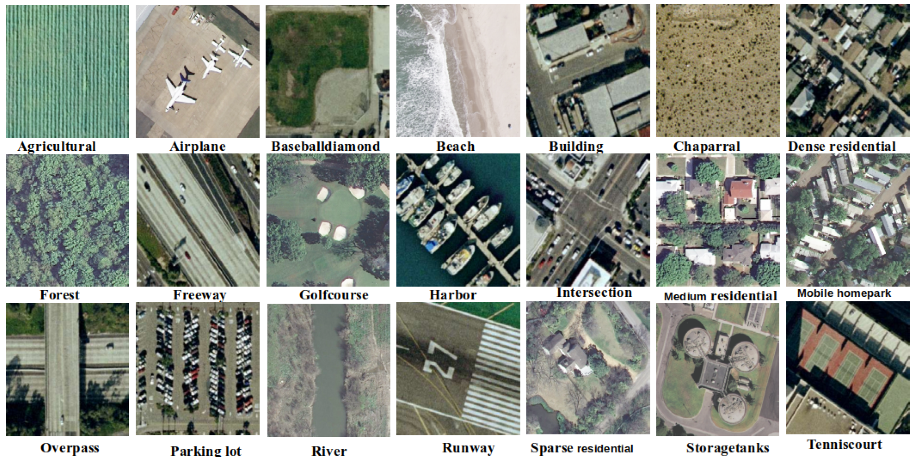
The UC Merced data set was selected as the first data set to evaluate the proposed method. As shown in Figure 2. the UC Merced data set contains 2100 images divided into 21 challenging categories with 100 images for each category. Each image under the data set contains $256\times 256\times 3$ pixels and 1 ft/pixel.

The UC Merced data set (constructed by aerial orthoimagery) is the most popular data set in the field of VHR image scene classification. It can be downloaded from the U.S Geological Survey (USGS) national map [28]. This data set has a high overlap between categories, such as sparse residential, medium residential, and dense residential, which mainly differ in the densities of the structures. Due to the small-scale scene categories and the sample numbers, there were sutured results in the UC Merced data set [38]. In order to alleviate these limitations, two large data sets were constructed (AID and NWPU-RESISC45) and were tested in this study as the second and third data sets, respectively.

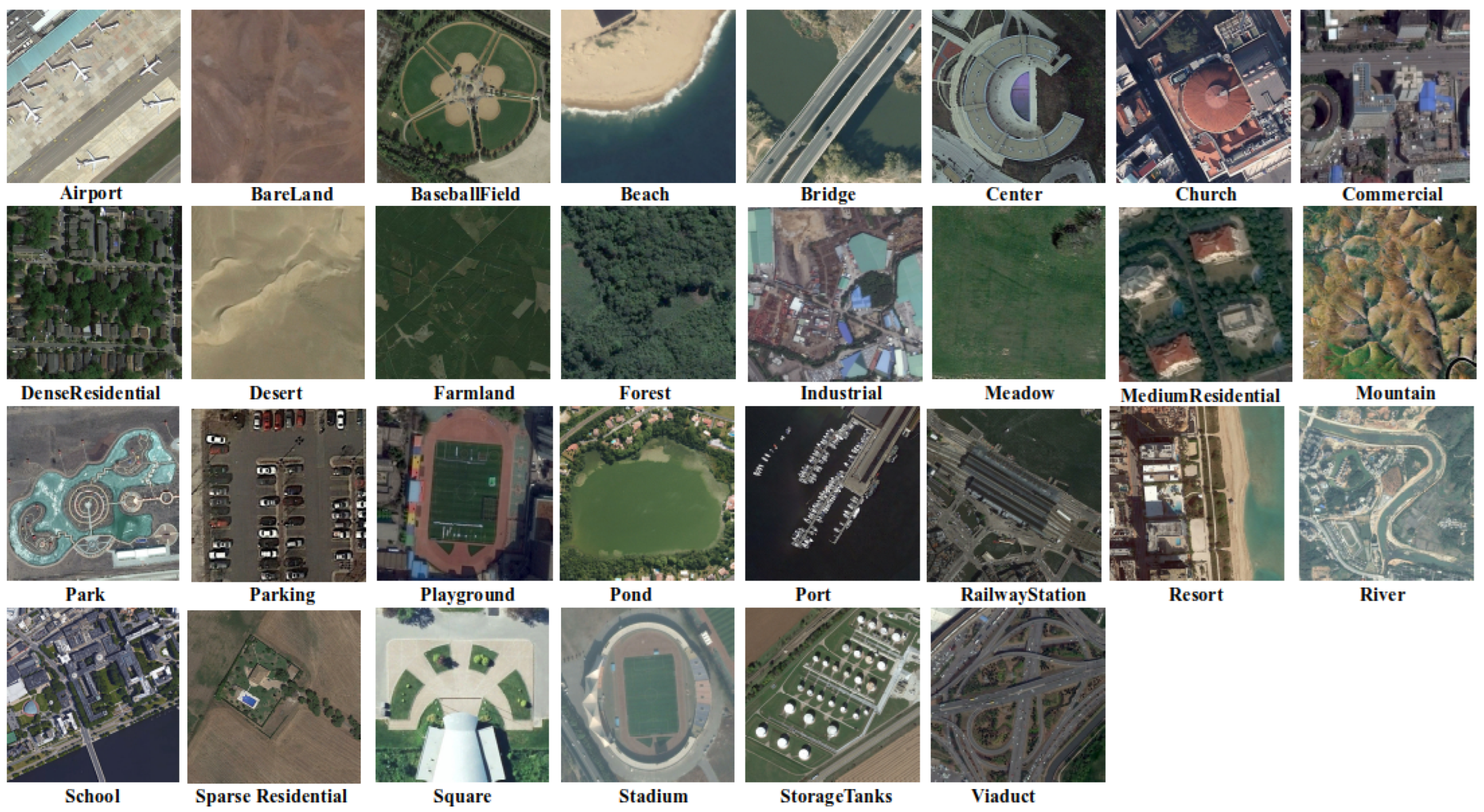
The second data set (AID) was created in [39] with the aim of renewing the VHR image scene classification challenges. This data set was constructed from a large Google Earth satellite, which has 10,000 samples distributed into 30 challenging categories: bare land, center, industrial, forest, school, mountain, church, square, stadium, farmland, airport, park, pond, baseball field, beach, river, bridge, meadow, commercial, sparse residential, dense residential, storage tanks, medium residential, railway station, playground, desert, port, resort, parking, and viaduct, as shown in Figure 3. Each image in this data set contains $600\times 600$ pixels with a spatial resolution varying from 8 m to $0.5$ m.

The third data set is named NWPU-RESISC45 [40]. This is the largest data set in the field of VHR image scene classification. This data set was constructed via Google Earth by experts and researchers in the field of remote sensing image understanding. It contains 31,500 images distributed into 45 classes as shown in Figure 4, where each class is composed of 700 images, and each image contains $256\times 256\times 3$ pixels with a spatial resolution varying from 30 to $0.2$ m per pixel.

3.2. Experimental

To evaluate and analyze the performance of the proposed method, we tested it on the three different data sets described above. We selected the transformer–encoder layers by applying the ViT model to extract the descriptive features from each image scene, where we considered the encoder layers (as deep high-level feature descriptors) as the final feature representations of the input images. Then, we applied the co-selection method to compute the important features and the images. In fact, in the training set, some images were not useful (abnormal); this could negatively affect the performance of the learning algorithm. The instance selection task is an efficient pre-processing step; it involves removing abnormal training instances (images) and reducing the overall dimensionality of a data set. In the classification task, we used the LIBSVM library [41] to separately classify each feature set, then used a probability fusion model established to compute the final accuracy. The classification performance was measured by $A=\frac{N_c}{N_t}$, where $N_c$ denotes the number of correctly classified samples in the tested samples and $N_t$ denotes the total number of testing samples. We evaluated the final classification performance with the average accuracy $\overline{A}$ over 10 runs for each data set, where, in each run, we randomly selected the training and testing samples.

3.3. UC Merced Data Set

In order to assess the scene classification performance of the proposed approach on the UC Merced data set, we selected 80 images per class for the training task and the remaining 20 for evaluation using the same experimental setup as cited in [42]. In terms of classification performance, we compared the results achieved from different feature descriptors extracted with four pre-trained ViT models, and the final performance computed by the fusion of these features, as shown in

Table 2. Comparison with different ViT features on the UC Merced data set.

Models	Accuracy
	50% Training Ratio	80% Training Ratio
ViT8b	$97.41\pm 0.00158$	$97.59\pm 0.00067$
ViT16b	$96.91\pm 0.0029$	$98.78\pm 0.00076$
ViT8s	$96.62\pm 0.0014$	$98.08\pm 0.00383$
ViT16s	$95.81\pm 0.00065$	$98.07\pm 0.00296$
Fusion	97.7 ± 0.00113	99.49 ± 0.001

.

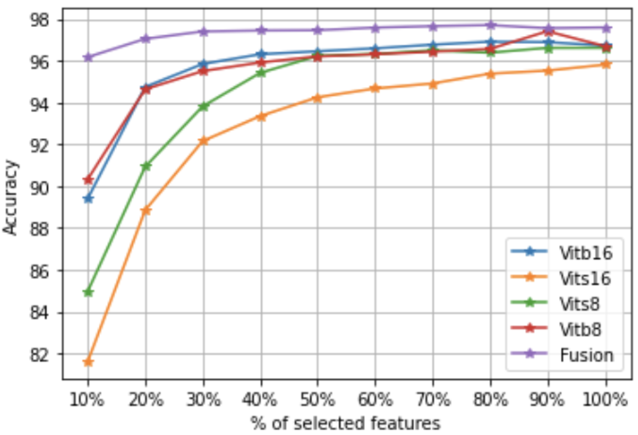
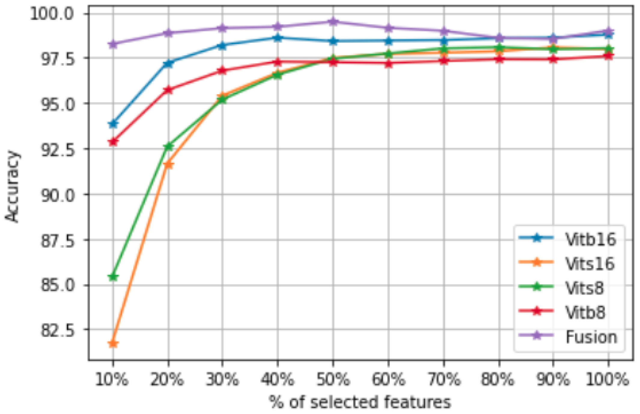
In order to study the sensitivity of important features, we varied their values over a wide range, from $10\%$ to $100\%$, as shown in Figure 5 and Figure 6. The number of important features ($50\%$) achieved the highest accuracy based on the fusion of all ViT features.

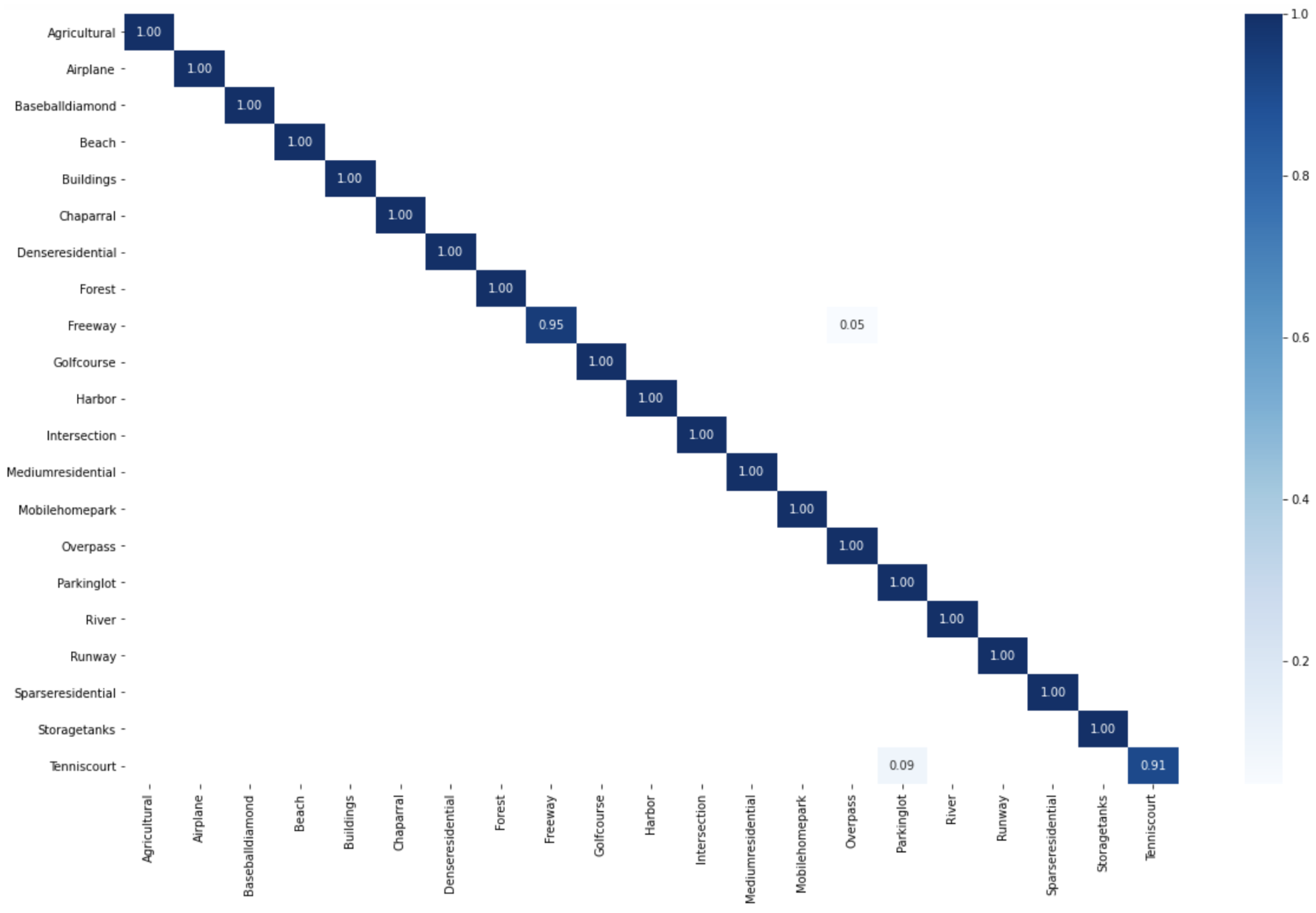
The confusion matrix performance for each category of the UC Merced data set; each data set with a different convolutional bag is shown in Figure 7 and Figure 8.

We compared the proposed framework with state-of-the-art VHR image scene classification works based on deep learning approaches on the UC Merced data set as shown in

Table 3. Overall accuracy and standard deviation of the proposed method and comparison approaches on the UC Merced data set.

Methods	80% Train	50% Train
TEX-Net-LF [43]	$96.62\pm 0.49$	$95.89\pm 0.37$
Fine-tuned GoogLeNet [29]	$97.78\pm 0.97$	-
MCNN [44]	$96.66\pm 0.90$	-
MSCP [45]	$98.36\pm 0.58$	-
ADFF [46]	$98.81\pm 0.51$	-
MLFF_WWA [47]	$98.46$	-
Two-Stream Fusion [48]	$98.02\pm 1.03$	$96.97\pm 0.75$
ARCNet-VGG16 [49]	$99.12\pm 0.40$	$96.81\pm 0.14$
ACR _MLFF [51]	$99.37\pm 0.15$	$97.99\pm 0.26$
LCPP [50]	$97.54\pm 1.02$	-
PROPOSED	99.49 ± 0.001	97.90 ± 0.00113

. Including the method described in [43], the fine-tuned GoogLeNet was followed by linear SVM introduced in [29], VHR scene classification based on multiscale convolutional neural network [44], multilayer stacked covariance pooling for remote sensing scene classification [45], multiple fisher vector feature aggregation-based methods [46], multilayer feature fusion method for VHR images classification [47], two-stream deep fusion framework for high-resolution aerial scene classification [48], scene classification with recurrent attention of VHR remote sensing images [49], a multi-level convolution pyramid semantic fusion framework for high-resolution remote sensing image scene classification and annotation [50], and multilevel feature fusion networks with adaptive channel dimensionality reduction for remote sensing scene classification [51]. In terms of overall classification accuracy, the results in Table 3 clearly show that the co-selection of vision transformer features and images outperforms all the other methods.

3.4. AID Data Set

The sutured VHR scene classification performance on the UC Merced data set encourages researchers to construct more challenging data sets to advance aerial scene classification problems. The AID data set created by Xia et al. [39] is illustrated above. To evaluate the classification results of this study on the AID data set, we selected $50\%$ of the labeled images from each class for training and the remaining second half for testing the same using a setup in [39]. In terms of overall accuracy, we compared the different features computed from ViT8b, ViT16b, ViT8s, and ViT16s, with the final overall accuracy achieved by the fusion of these features as noted in

Table 4. Comparison with different ViT features on the AID data set.

Models	Accuracy
	20% Training Ratio	50% Training Ratio
ViT8b	$93.28\pm 0.00050$	$95.88\pm 0.00$
ViT16b	$92.60\pm 0.00$	$95.25\pm 0.00018$
ViT8s	$92.13\pm 0.00048$	$94.35\pm 0.00375$
ViT16s	$90.63\pm 0.00044$	$93.62\pm 0.00139$
Fusion	94.54 ± 0.00071	96.75 ± 0.00104

.

In order to study the sensitivity of important features on the AID data set, we varied their values over a wide range, from $10\%$ to $100\%$, as shown in Figure 9 and Figure 10. The number of important features ($80\%$) achieved the highest accuracy based on the fusion of all ViT features.

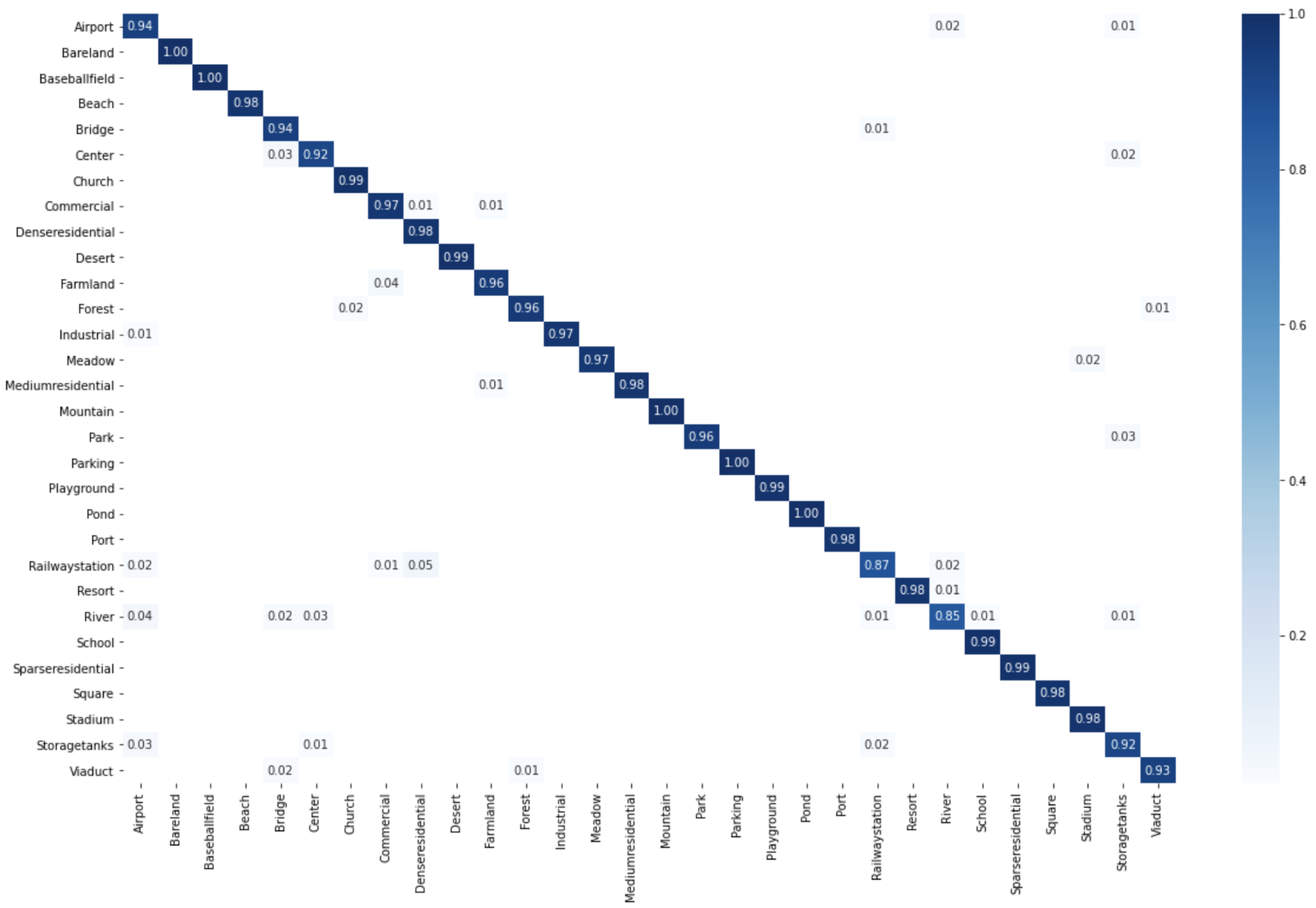
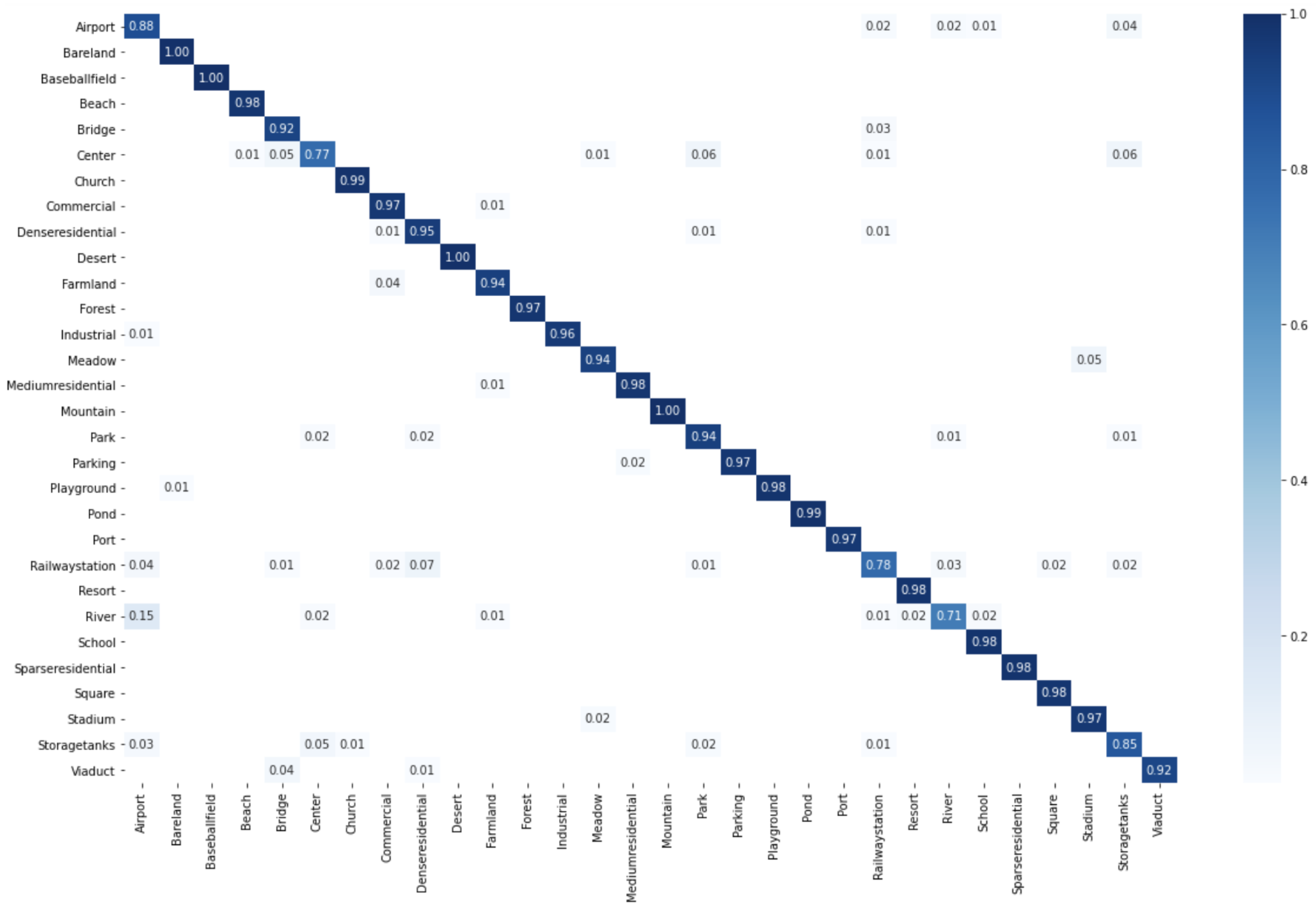
The confusion matrix performances for each category of the AID data set are shown in Figure 11, for which the training ratio was set to $50\%$, and in Figure 12 with the training ratio is equal to $20\%$.

Table 5. Overall accuracy and standard deviation of the proposed method and comparison approaches on the AID data set.

Methods	50% Train	20% Train
VGG-VD-16 [39]	$89.64\pm 0.36$	-
DCA fusion [34]	$91.87\pm 0.36$	-
Two Stream Fusion [48]	$94.57\pm 0.25$	$92.32\pm 0.41$
ACR _MLFF [51]	$95.06\pm 0.33$	$92.73\pm 0.12$
ARCNet-VGG16 [49]	$93.10\pm 0.55$	$88.75\pm 0.40$
LGFFE [52]	$90\pm 0.01$	$90.83\pm 0.55$11
LCPP [50]	$93.12\pm 0.28$	$90.96\pm 0.33$
PROPOSED	96.932 ± 0.00024	94.625 ± 0.0001

lists the performance comparisons of the proposed method on the AID data set, for several methods, including the original paper of this benchmark [39], which represent the image scenes with high-level feature descriptors using pre-trained CNN models, CaffeNet, VGG-VD-16, and GoogLeNet, deep feature fusion for remote sensing image classification [34], two-stage deep feature fusion for scene classification [48], multilevel feature fusion network with adaptive channel dimensionality reduction for remote sensing scene classification [51], scene classification with attention recurrent convolutional network [49], efficient end-to-end local–global fusion feature extraction (LGFFE) for VHR image classification [52], and a multi-level convolution pyramid semantic fusion framework for high-resolution remote sensing image scene classification and annotation [50]. The experimental results shown in

Table 6. Comparison with different ViT features on the NWPU-RESISC45 data set.

Models	Accuracy
	10% Training Ratio	20% Training Ratio
ViT8b	$87.53\pm 0.00052$	$90.26\pm 0.00005$
ViT16b	$87.19\pm 0.00002$	$89.82\pm 0.0$
ViT8s	$85.30\pm 0.00103$	$88.14\pm 0.00039$
ViT16s	$84.23\pm 0.00002$	$87.53\pm 0.00009$
Fusion	90.89 ± 0.0011	92.23 ± 0.0005

clearly demonstrate that our method performed well.

3.5. NWPU-RESISC45 Data Set

In order to evaluate the classification accuracy of the NWPU-RESISC45 data set, we followed the same method as the experiments cited in [40], where we selected 10 samples per category for training (70 training images from each class) and 90 samples for testing tasks (630 images per class). Similar to the experiments described above for three data sets, we compared the performances between the different ViT features extracted from different models: ViT8b, ViT16b, ViT8s, and ViT16b, and the final overall accuracies achieved by the fusion of these features, as noted in Table 6.

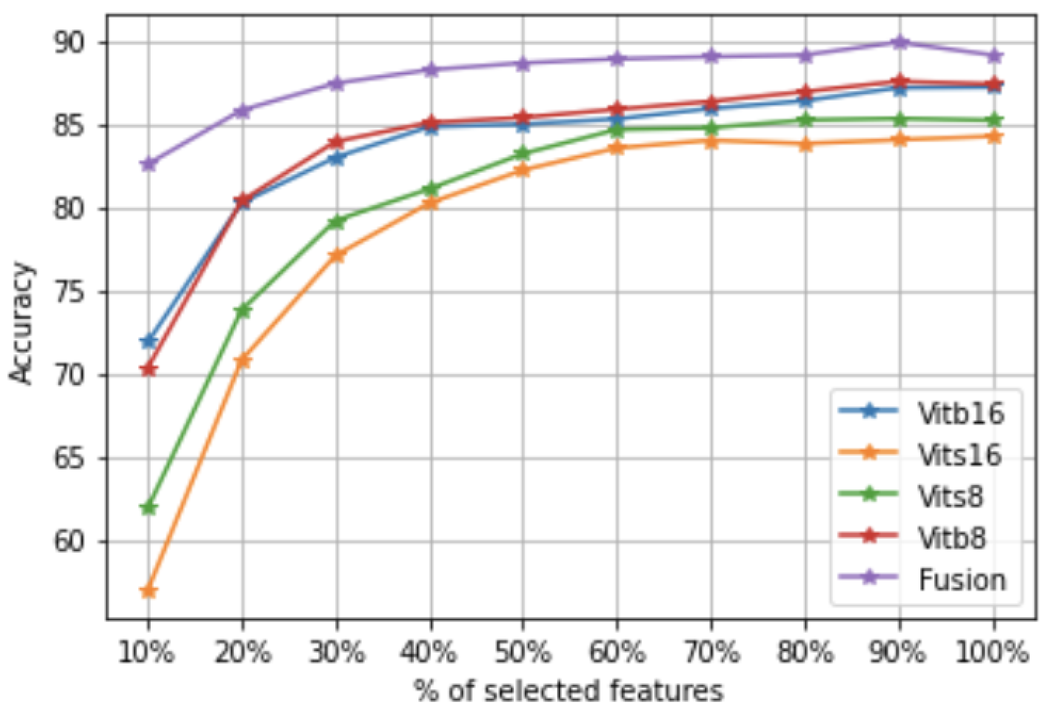
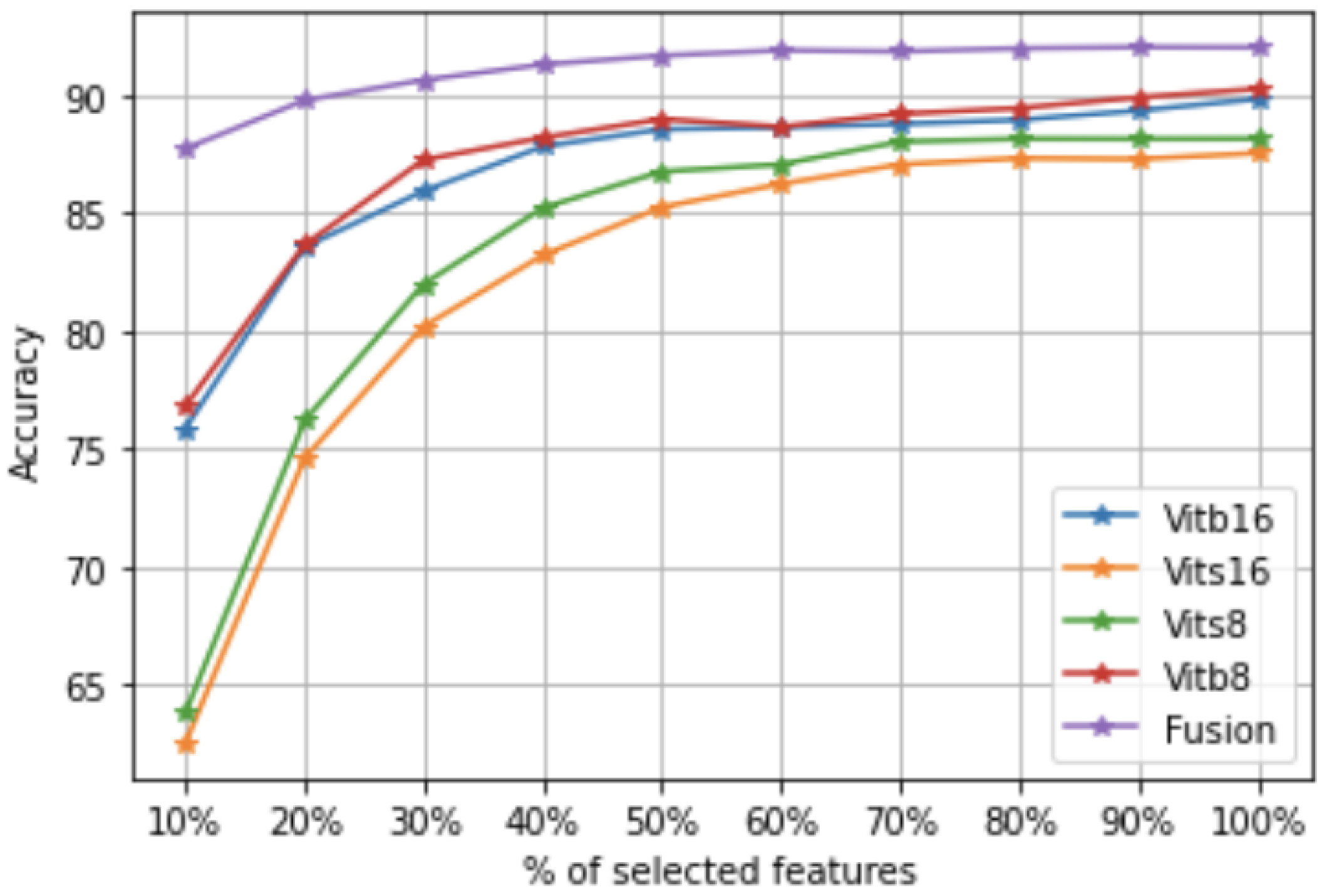
To study the sensitivity of important features on the NWPU-RESISC45 data set, we varied their values over a wide range from 10% to 100%, as shown in Figure 13 and Figure 14. The number of important features ($80\%$) achieved the highest accuracy based on the fusion of all ViT features.

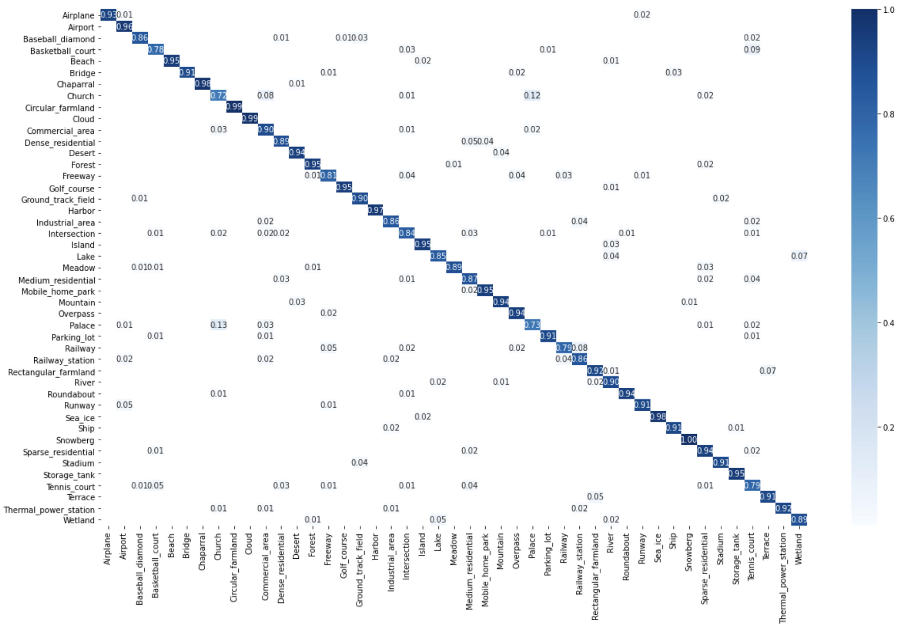
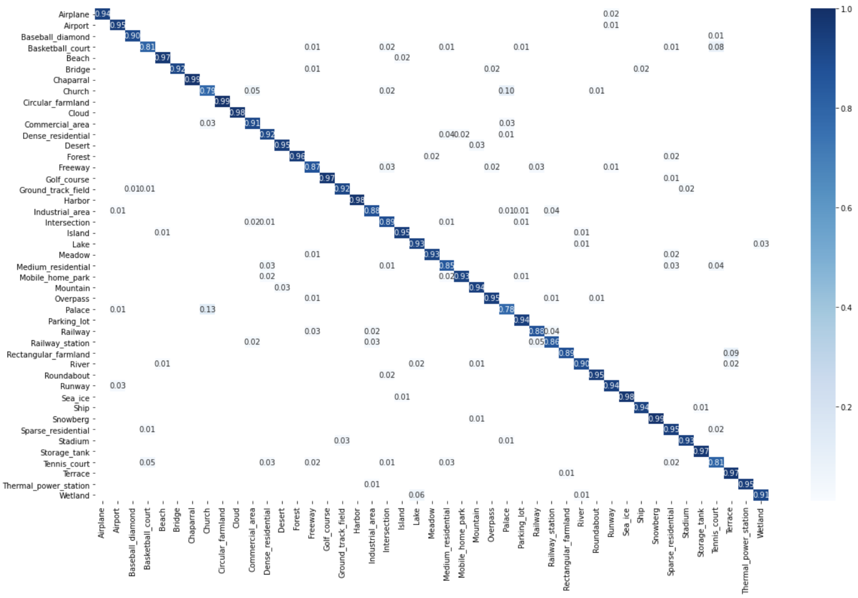
The confusion matrix performances for each category of the NWPU-RESISC45 data set are shown in Figure 15, for which the training ratio was set to $10\%$, and in Figure 16, with the training ratio equal to $20\%$.

Table 7. Overall accuracy and standard deviatio of the proposed method and comparison approaches on the NWPU-RESISC45 data set.

Methods	Training Ratios
	10 % Train	20% Train
AlexNet [40]	$76.69\pm 0.21$	$79.85\pm 0.13$
RAN [53]	$88.79\pm 0.53$	$91.40\pm 0.30$
GLANet [54]	$89.50\pm 0.26$	$91.50\pm 0.17$
ACR _MLFF [51]	90.01 ± 0.33	92.45 ± 0.20
T_CNN [55]	$90.25\pm 0.55$	93.05 ± 0.12
PROPOSED	90.89 ± 0.00011	$92.23\pm 0.00051$

presents the overall accuracy comparisons of the proposed method on the NWPU-RESISC45 data set with several aerial image scene classification approaches, including the original work of this data set [40], where the image scene is described with different feature descriptors (low-level, mid-level, and high-level) features. In this study, we only compared the achieved performances with high-level features, which used pre-trained CNN models, AlexNet, VGG-VD-16, GoogLeNet, and remote sensing image scenes based on attention residual network classification [53]. The experimental results shown in Table 7 demonstrate that our method performed well.

3.6. Ablation Study

In this subsection, an ablation study on the proposed method is conducted with co-selection and without co-selection. We evaluate the co-selection of vision transformer features by considering all feature and sample parts, i.e., we disable features and instance selections. Then, we consider the feature and image selection parts. The ablation results over the three data sets in terms of accuracy are shown in

Table 8. Ablation study of the proposed method on the three data sets.

	AID	NWPU	UC Merced
With Co-Selection	94.63	89.70	97.70
Without Co-Selection	94.02	88.45	96.92

.

4. Conclusions

In this paper, a new method for aerial image scene classification was developed. The proposed study is based on the pre-trained VIT model as a deep feature extractor. In order to generate global features for image scene representation, the extracted features from four different VIT models were fused. Based on the similarity of preserving the whole VHR image data set, we dropped anomalous features and images that degraded the classification accuracy. In fact, in the training set, some images were not useful, as they could have negatively affected the performance of the learning algorithms. The instance selection task is an efficient pre-processing step that involves removing unnecessary training instances (images) and reducing the overall dimensionality of a data set. Our approach allows us to select the most important features and images to facilitate the classification step. For this, our algorithm sorts the features/images according to their weights calculated during the algorithm through the R and Q matrices. At the end of the proposed algorithm, the user can sort the features and images according to the weights and take only the most important. The experimental results from different remote sensing image scenes demonstrate that the pre-trained ViT model can provide useful features for VHR image scene classification.

References

1. Oliva, A.; Torralba, A. Modeling the shape of the scene: A holistic representation of the spatial envelope. Int. J. Comput. Vis. 2001, 42, 145–175. [Google Scholar] [CrossRef]
2. Ojala, T.; Pietikainen, M.; Maenpaa, T. Multiresolution gray-scale and rotation invariant texture classification with local binary patterns. IEEE Trans. Pattern Anal. Mach. Intell. 2002, 24, 971–987. [Google Scholar] [CrossRef]
3. Swain, M.J.; Ballard, D.H. Color indexing. Int. J. Comput. Vis. 1991, 7, 11–32. [Google Scholar] [CrossRef]
4. Lowe, D.G. Object recognition from local scale-invariant features. In Proceedings of the Seventh IEEE International Conference on Computer Vision, Kerkyra, Greece, 20–27 September 1999; Volume 2, pp. 1150–1157. [Google Scholar]
5. Dalal, N.; Triggs, B. Histograms of oriented gradients for human detection. In Proceedings of the 2005 IEEE Computer Society Conference on Computer Vision and Pattern Recognition (CVPR’05), San Diego, CA, USA, 20–25 June 2005; Volume 1, pp. 886–893. [Google Scholar]
6. Yang, Y.; Newsam, S. Comparing SIFT descriptors and Gabor texture features for classification of remote sensed imagery. In Proceedings of the 2008 15th IEEE International Conference on Image Processing, San Diego, CA, USA, 12–15 October 2008; pp. 1852–1855. [Google Scholar]
7. dos Santos, J.A.; Penatti, O.A.B.; da Silva Torres, R. Evaluating the Potential of Texture and Color Descriptors for Remote Sensing Image Retrieval and Classification. In Proceedings of the VISAPP, Angers, France, 17–21 May 2010. [Google Scholar]
8. Risojević, V.; Momić, S.; Babić, Z. Gabor descriptors for aerial image classification. In Proceedings of the International Conference on Adaptive and Natural Computing Algorithms, Ljubljana, Slovenia, 14–16 April 2011; pp. 51–60. [Google Scholar]
9. Avramović, A.; Risojević, V. Block-based semantic classification of high-resolution multispectral aerial images. Signal Image Video Process. 2016, 10, 75–84. [Google Scholar] [CrossRef]
10. Chen, X.; Fang, T.; Huo, H.; Li, D. Measuring the effectiveness of various features for thematic information extraction from very high resolution remote sensing imagery. IEEE Trans. Geosci. Remote Sens. 2015, 53, 4837–4851. [Google Scholar] [CrossRef]
11. Luo, B.; Jiang, S.; Zhang, L. Indexing of remote sensing images with different resolutions by multiple features. IEEE J. Sel. Top. Appl. Earth Obs. Remote Sens. 2013, 6, 1899–1912. [Google Scholar] [CrossRef]
12. Luo, B.; Aujol, J.F.; Gousseau, Y.; Ladjal, S. Indexing of satellite images with different resolutions by wavelet features. IEEE Trans. Image Process. 2008, 17, 1465–1472. [Google Scholar]
13. Luo, B.; Aujol, J.F.; Gousseau, Y. Local scale measure from the topographic map and application to remote sensing images. Multiscale Model. Simul. 2009, 8, 1–29. [Google Scholar] [CrossRef] [Green Version]
14. Qi, K.; Wu, H.; Shen, C.; Gong, J. Land-use scene classification in high-resolution remote sensing images using improved correlatons. IEEE Geosci. Remote Sens. Lett. 2015, 12, 2403–2407. [Google Scholar]
15. Cheng, G.; Han, J.; Zhou, P.; Guo, L. Multi-class geospatial object detection and geographic image classification based on collection of part detectors. ISPRS J. Photogramm. Remote Sens. 2014, 98, 119–132. [Google Scholar] [CrossRef]
16. Drăguţ, L.; Blaschke, T. Automated classification of landform elements using object-based image analysis. Geomorphology 2006, 81, 330–344. [Google Scholar] [CrossRef]
17. Zhang, J.; Li, T.; Lu, X.; Cheng, Z. Semantic classification of high-resolution remote-sensing images based on mid-level features. IEEE J. Sel. Top. Appl. Earth Obs. Remote Sens. 2016, 9, 2343–2353. [Google Scholar] [CrossRef]
18. Cui, S.; Schwarz, G.; Datcu, M. Remote sensing image classification: No features, no clustering. IEEE J. Sel. Top. Appl. Earth Obs. Remote Sens. 2015, 8, 5158–5170. [Google Scholar] [CrossRef] [Green Version]
19. Sivic, J.; Zisserman, A. Video Google: A text retrieval approach to object matching in videos. In Proceedings of the Computer Vision, IEEE International Conference on. IEEE Computer Society, Nice, France, 13–16 October 2003; Volume 3, p. 1470. [Google Scholar]
20. Cheng, G.; Guo, L.; Zhao, T.; Han, J.; Li, H.; Fang, J. Automatic landslide detection from remote-sensing imagery using a scene classification method based on BoVW and pLSA. Int. J. Remote Sens. 2013, 34, 45–59. [Google Scholar] [CrossRef]
21. Zhao, L.; Tang, P.; Huo, L. Feature significance-based multibag-of-visual-words model for remote sensing image scene classification. J. Appl. Remote Sens. 2016, 10, 035004. [Google Scholar] [CrossRef]
22. Wu, H.; Liu, B.; Su, W.; Zhang, W.; Sun, J. Hierarchical coding vectors for scene level land-use classification. Remote Sens. 2016, 8, 436. [Google Scholar] [CrossRef] [Green Version]
23. Zhang, Y.; Sun, X.; Wang, H.; Fu, K. High-resolution remote-sensing image classification via an approximate earth mover’s distance-based bag-of-features model. IEEE Geosci. Remote Sens. Lett. 2013, 10, 1055–1059. [Google Scholar] [CrossRef]
24. Cheng, G.; Han, J.; Guo, L.; Liu, Z.; Bu, S.; Ren, J. Effective and efficient mid-level visual elements-oriented land-use classification using VHR remote sensing images. IEEE Trans. Geosci. Remote Sens. 2015, 53, 4238–4249. [Google Scholar] [CrossRef] [Green Version]
25. Hu, F.; Xia, G.S.; Hu, J.; Zhang, L. Transferring deep convolutional neural networks for the scene classification of high-resolution remote sensing imagery. Remote Sens. 2015, 7, 14680–14707. [Google Scholar] [CrossRef] [Green Version]
26. Deng, J.; Berg, A.; Satheesh, S.; Su, H.; Khosla, A.; Li, F. Imagenet Large Scale Visual Recognition Competition. ilsvrc2012. 2012. Available online: https://image-net.org/challenges/LSVRC/ (accessed on 15 March 2020).
27. Zhang, F.; Du, B.; Zhang, L. Scene classification via a gradient boosting random convolutional network framework. IEEE Trans. Geosci. Remote Sens. 2015, 54, 1793–1802. [Google Scholar] [CrossRef]
28. Yang, Y.; Newsam, S. Bag-of-visual-words and spatial extensions for land-use classification. In Proceedings of the 18th SIGSPATIAL International Conference on Advances in Geographic Information Systems, San Jose, CA, USA, 2–5 November 2010; pp. 270–279. [Google Scholar]
29. Nogueira, K.; Penatti, O.A.; Dos Santos, J.A. Towards better exploiting convolutional neural networks for remote sensing scene classification. Pattern Recognit. 2017, 61, 539–556. [Google Scholar] [CrossRef] [Green Version]
30. Othman, E.; Bazi, Y.; Alajlan, N.; Alhichri, H.; Melgani, F. Using convolutional features and a sparse autoencoder for land-use scene classification. Int. J. Remote Sens. 2016, 37, 2149–2167. [Google Scholar] [CrossRef]
31. Vaswani, A.; Shazeer, N.; Parmar, N.; Uszkoreit, J.; Jones, L.; Gomez, A.N.; Kaiser, Ł.; Polosukhin, I. Attention is all you need. In Proceedings of the Advances in Neural Information Processing Systems, Long Beach, CA, USA, 4–9 December 2017; Volume 30. [Google Scholar]
32. Tsai, Y.H.H.; Bai, S.; Liang, P.P.; Kolter, J.Z.; Morency, L.P.; Salakhutdinov, R. Multimodal transformer for unaligned multimodal language sequences. In Proceedings of the Association for Computational Linguistics Meeting, Florence, Italy, 28 July–2 August 2019; Volume 2019, p. 6558. [Google Scholar]
33. Dosovitskiy, A.; Beyer, L.; Kolesnikov, A.; Weissenborn, D.; Zhai, X.; Unterthiner, T.; Dehghani, M.; Minderer, M.; Heigold, G.; Gelly, S.; et al. An image is worth 16x16 words: Transformers for image recognition at scale. arXiv 2020, arXiv:2010.11929. [Google Scholar]
34. Chaib, S.; Liu, H.; Gu, Y.; Yao, H. Deep feature fusion for VHR remote sensing scene classification. IEEE Trans. Geosci. Remote Sens. 2017, 55, 4775–4784. [Google Scholar] [CrossRef]
35. Benabdeslem, K.; Mansouri, D.E.K.; Makkhongkaew, R. sCOs: Semi-Supervised Co-Selection by a Similarity Preserving Approach. IEEE Trans. Knowl. Data Eng. 2022, 34, 2899–2911. [Google Scholar] [CrossRef]
36. Tang, J.; Liu, H. Coselect: Feature selection with instance selection for social media data. In Proceedings of the 2013 SIAM International Conference on Data Mining, Austin, TX, USA, 2–4 May 2013; pp. 695–703. [Google Scholar]
37. She, Y.; Owen, A.B. Outlier Detection Using Nonconvex Penalized Regression. J. Am. Stat. Assoc. 2011, 106, 626–639. [Google Scholar] [CrossRef] [Green Version]
38. Castelluccio, M.; Poggi, G.; Sansone, C.; Verdoliva, L. Land use classification in remote sensing images by convolutional neural networks. arXiv 2015, arXiv:1508.00092. [Google Scholar]
39. Xia, G.S.; Hu, J.; Hu, F.; Shi, B.; Bai, X.; Zhong, Y.; Zhang, L.; Lu, X. AID: A benchmark data set for performance evaluation of aerial scene classification. IEEE Trans. Geosci. Remote Sens. 2017, 55, 3965–3981. [Google Scholar] [CrossRef] [Green Version]
40. Cheng, G.; Han, J.; Lu, X. Remote sensing image scene classification: Benchmark and state of the art. Proc. IEEE 2017, 105, 1865–1883. [Google Scholar] [CrossRef] [Green Version]
41. Chang, C.C.; Lin, C.J. LIBSVM: A library for support vector machines. ACM Trans. Intell. Syst. Technol. 2011, 2, 1–27. [Google Scholar] [CrossRef]
42. Zhang, F.; Du, B.; Zhang, L. Saliency-guided unsupervised feature learning for scene classification. IEEE Trans. Geosci. Remote Sens. 2014, 53, 2175–2184. [Google Scholar] [CrossRef]
43. Anwer, R.M.; Khan, F.S.; Van De Weijer, J.; Molinier, M.; Laaksonen, J. Binary patterns encoded convolutional neural networks for texture recognition and remote sensing scene classification. ISPRS J. Photogramm. Remote Sens. 2018, 138, 74–85. [Google Scholar] [CrossRef] [Green Version]
44. Liu, Y.; Zhong, Y.; Qin, Q. Scene classification based on multiscale convolutional neural network. IEEE Trans. Geosci. Remote Sens. 2018, 56, 7109–7121. [Google Scholar] [CrossRef] [Green Version]
45. He, N.; Fang, L.; Li, S.; Plaza, A.; Plaza, J. Remote sensing scene classification using multilayer stacked covariance pooling. IEEE Trans. Geosci. Remote Sens. 2018, 56, 6899–6910. [Google Scholar] [CrossRef]
46. Li, B.; Su, W.; Wu, H.; Li, R.; Zhang, W.; Qin, W.; Zhang, S. Aggregated deep fisher feature for VHR remote sensing scene classification. IEEE J. Sel. Top. Appl. Earth Obs. Remote Sens. 2019, 12, 3508–3523. [Google Scholar] [CrossRef]
47. Ma, C.; Mu, X.; Lin, R.; Wang, S. Multilayer feature fusion with weight adjustment based on a convolutional neural network for remote sensing scene classification. IEEE Geosci. Remote Sens. Lett. 2020, 18, 241–245. [Google Scholar] [CrossRef]
48. Yu, Y.; Liu, F. A two-stream deep fusion framework for high-resolution aerial scene classification. Comput. Intell. Neurosci. 2018, 2018, 8639367. [Google Scholar] [CrossRef] [Green Version]
49. Wang, Q.; Liu, S.; Chanussot, J.; Li, X. Scene classification with recurrent attention of VHR remote sensing images. IEEE Trans. Geosci. Remote Sens. 2018, 57, 1155–1167. [Google Scholar] [CrossRef]
50. Sun, X.; Zhu, Q.; Qin, Q. A multi-level convolution pyramid semantic fusion framework for high-resolution remote sensing image scene classification and annotation. IEEE Access 2021, 9, 18195–18208. [Google Scholar] [CrossRef]
51. Wang, X.; Duan, L.; Shi, A.; Zhou, H. Multilevel feature fusion networks with adaptive channel dimensionality reduction for remote sensing scene classification. IEEE Geosci. Remote Sens. Lett. 2021, 19, 1–5. [Google Scholar] [CrossRef]
52. Lv, Y.; Zhang, X.; Xiong, W.; Cui, Y.; Cai, M. An end-to-end local-global-fusion feature extraction network for remote sensing image scene classification. Remote Sens. 2019, 11, 3006. [Google Scholar] [CrossRef] [Green Version]
53. Fan, R.; Wang, L.; Feng, R.; Zhu, Y. Attention based residual network for high-resolution remote sensing imagery scene classification. In Proceedings of the IGARSS 2019—2019 IEEE International Geoscience and Remote Sensing Symposium, Yokohama, Japan, 28 July–2 August 2019; pp. 1346–1349. [Google Scholar]
54. Guo, Y.; Ji, J.; Lu, X.; Huo, H.; Fang, T.; Li, D. Global-local attention network for aerial scene classification. IEEE Access 2019, 7, 67200–67212. [Google Scholar] [CrossRef]
55. Wang, W.; Chen, Y.; Ghamisi, P. Transferring CNN With Adaptive Learning for Remote Sensing Scene Classification. IEEE Trans. Geosci. Remote Sens. 2022, 60, 1–18. [Google Scholar] [CrossRef]
Figure 1. Overall architecture of the proposed method.
Remotesensing 14 05817 g001
Figure 2. Example images associated with 21 land use categories in the UC Merced data set.
Remotesensing 14 05817 g002
Figure 3. Example images associated with 30 land use classes in the AID data set.
Remotesensing 14 05817 g003
Figure 4. Example images associated with 45 land use categories in the NWPU RESISC45 data set.
Remotesensing 14 05817 g004
Figure 5. Rate of important feature effects on the classification accuracy of the UC Merced data set with 50 % of randomly selected images per class.
Remotesensing 14 05817 g005
Figure 6. Rate of important feature effects on the classification accuracy of the UC Merced data set with 80 % of randomly selected images per class.
Remotesensing 14 05817 g006
Figure 7. Confusion matrix of our method under the 80 % training ratio and 50 % of important features on the UC Merced data set.
Remotesensing 14 05817 g007
Figure 8. Confusion matrix of our method under the 50 % training ratio and 50 % of important features on the UC Merced data set.
Remotesensing 14 05817 g008
Figure 9. The rate of important feature effects on the classification accuracy of the AID data set with 20 % of randomly selected images per class.
Remotesensing 14 05817 g009
Figure 10. Rate of important feature effects on the classification accuracy of the AID data set with 50 % of randomly selected images per class.
Remotesensing 14 05817 g010
Figure 11. Confusion matrix of our method under the 50 % training ratio and 90 % of important features on the AID data set.
Remotesensing 14 05817 g011
Figure 12. Confusion matrix of our method under the 20 % training ratio and 90 % of important features on the AID data set.
Remotesensing 14 05817 g012
Figure 13. Rate of important feature effects on the classification accuracy of the NWPU-RESISC45 data set with 10 % randomly selected images per class.
Remotesensing 14 05817 g013
Figure 14. Rate of important feature effects on the classification accuracy of the NWPU-RESISC45 data set with 20 randomly selected images per class.
Remotesensing 14 05817 g014
Figure 15. Confusion matrix of our method under the 10 % training ratio and 90 % of features on the NWPU data set.
Remotesensing 14 05817 g015
Figure 16. Confusion matrix of our method under the 20 % training ratio 90 % of features on the NWPU data set.
Remotesensing 14 05817 g016