Article

SEG-ESRGAN: A Multi-Task Network for Super-Resolution and Semantic Segmentation of Remote Sensing Images

by
Luis Salgueiro
1,
Javier Marcello
2 and
Verónica Vilaplana
1,*
1
Department of Signal Theory and Communications, Technical University of Catalonia, 08034 Barcelona, Spain
2
Instituto de Oceanografía y Cambio Global, IOCAG, Unidad Asociada ULPGC-CSIC, 35017 Las Palmas de Gran Canaria, Spain
*
Author to whom correspondence should be addressed.
Remote Sens. 2022, 14(22), 5862; https://doi.org/10.3390/rs14225862
Submission received: 8 October 2022 / Revised: 4 November 2022 / Accepted: 17 November 2022 / Published: 19 November 2022
(This article belongs to the Special Issue Remote Sensing Image Super Resolution)

Abstract

:
The production of highly accurate land cover maps is one of the primary challenges in remote sensing, which depends on the spatial resolution of the input images. Sometimes, high-resolution imagery is not available or is too expensive to cover large areas or to perform multitemporal analysis. In this context, we propose a multi-task network to take advantage of the freely available Sentinel-2 imagery to produce a super-resolution image, with a scaling factor of 5, and the corresponding high-resolution land cover map. Our proposal, named SEG-ESRGAN, consists of two branches: the super-resolution branch, that produces Sentinel-2 multispectral images at 2 m resolution, and an encoder–decoder architecture for the semantic segmentation branch, that generates the enhanced land cover map. From the super-resolution branch, several skip connections are retrieved and concatenated with features from the different stages of the encoder part of the segmentation branch, promoting the flow of meaningful information to boost the accuracy in the segmentation task. Our model is trained with a multi-loss approach using a novel dataset to train and test the super-resolution stage, which is developed from Sentinel-2 and WorldView-2 image pairs. In addition, we generated a dataset with ground-truth labels for the segmentation task. To assess the super-resolution improvement, the PSNR, SSIM, ERGAS, and SAM metrics were considered, while to measure the classification performance, we used the IoU, confusion matrix and the F1-score. Experimental results demonstrate that the SEG-ESRGAN model outperforms different full segmentation and dual network models (U-Net, DeepLabV3+, HRNet and Dual_DeepLab), allowing the generation of high-resolution land cover maps in challenging scenarios using Sentinel-2 10 m bands.

1. Introduction

The application of Deep Learning (DL) in Remote Sensing (RS) for Earth Observation applications has contributed with significant advances in many fields, being Land-Use/Land-Cover (LULC) and data fusion the most relevant [1]. Moreover, the learning capacity of DL models have attracted the RS community in generating automated workflows, extracting high-level representations from raw data that are transformed to achieve excellent performance in the production of valuable assets [2].
One fundamental feature of RS images is the spatial resolution, which is defined as the minimum distance in which two separated objects can be distinguished [3]. Nowadays, many platforms, managed by public or private agencies, provide data with different spatial resolutions, where a higher resolution image has better detailed objects that can result in a more accurate segmentation map. A major problem is that high-resolution (HR) images are not always available with the specific characteristic requested, or obtaining them may represent a considerable economic barrier to circumvent.
One of the main characteristics that have driven the blooming in research and application in RS is the availability of open-access satellite data, providing free-of-charge imagery, such as those produced by the Copernicus Program (https://scihub.copernicus.eu/dhus/#/home, accessed on 7 October 2022), being the Sentinel-2 the foremost exponent of the constellation of multispectral medium- and high-resolution satellites available. The Copernicus Sentinel-2 satellites are two identical platforms, orbiting the Earth with a high revisit time and capable of providing multiSpectral (MS) images with a considerable surface coverage and different spatial resolutions (at 10, 20 and 60 m), covering the Visible and Near-Infrared Spectrum (VIS-NIR).
In computer vision, Semantic Segmentation (SS) assigns semantics labels to the pixels of an image [4]. In the context of LULC, the labels correspond to a semantic class and having an HR image for this purpose is essential for achieving good accuracy in the segmentation [5]. Therefore, to take advantage of the free usability of the Copernicus program, we propose the use of super-resolution techniques to assist with the segmentation task by enhancing the details of the 10 m bands provided by the Sentinel-2 satellite.
When a panchromatic channel with higher spatial detail is not available, super-resolution (SR) methods can provide a suitable alternative to promote the use of enhanced bands. For this reason, in the last decade, the improvement of the spatial resolution of RS images has been a very active research area, aiming to reduce cost when addressing studies requiring imagery with a very high spatial resolution that usually represents a considerable budget on any project. Most common approaches are based on Convolutional Neural Networks (CNN) and Generative Adversarial Networks (GAN), achieving outstanding results on different RS data.
Many authors have also tackled the idea of applying DL semantic segmentation models to different RS datasets, mainly using hyperspectral or aerial images due the spectral and spatial characteristics. However, in this work, we extend our analysis to works that have applied SR as a preprocessing step or even combined with SR to improve performance in generating land cover maps or other RS applications.
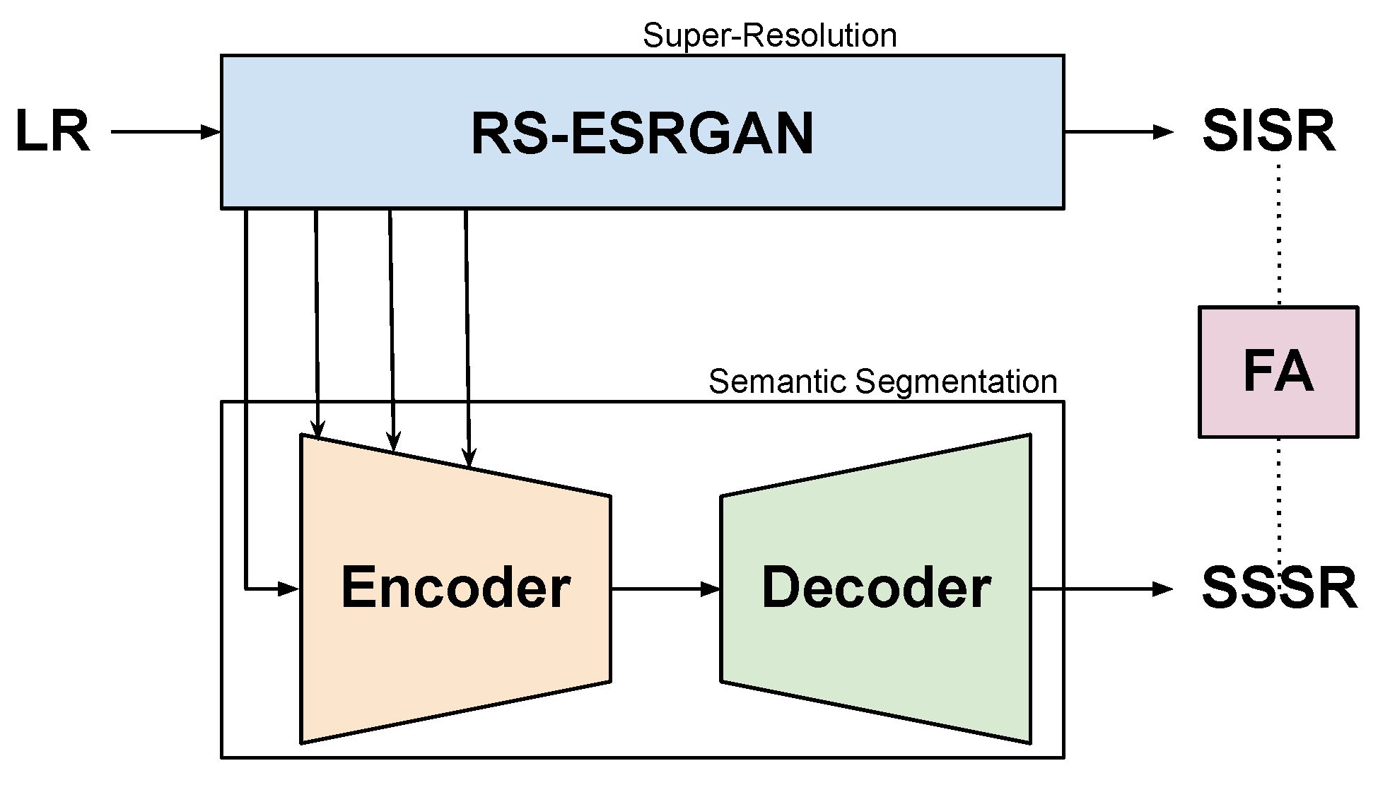
The key point of our work is a multi-task network approach, which is inspired by [6]. This approach consists in predicting an SR image with its corresponding HR land-cover map from a low-resolution (LR) Sentinel-2 image. Predictions are made simultaneously in a multi-task fashion by employing two dedicated branches in the network architecture that collaborate in training to maximize their performance. Our model, named SEG-ESRGAN (Segmentation Enhanced Super-resolution Generative Adversarial Network), takes our previous proposal RS-ESRGAN [7] for super-resolution and extends this model coupling an encoder–decoder architecture to perform the segmentation task, i.e., to produce a Semantic Segmentation Super-Resolution (SSSR) map. The training was completed in a supervised manner, using very-high-resolution imagery and its LULC map, which was obtained from a WorldView-2 satellite. In this manner, we leverage the 10 m bands from Sentinel-2 to a challenging 2 m of spatial resolution (scaling factor of 5) with a substantial improvement on the land cover classification task, which, to the best of our knowledge, was not tackled before.
The organization of this paper is as follows: Section 2 presents the relevant works related to the application of Deep Learning to SR, SS and multi-tasking methods in RS. In Section 3, we present the materials and methods, describing the dataset, the model, training details and quantitative metrics used for evaluation. In Section 4, we present the experimental results with the discussion in Section 5. Finally, we present our conclusions in Section 6.

2. Related Works

2.1. Super-Resolution

Considered as an ill-posed problem by many authors [8,9], SR seeks to recover an HR version of an LR image by learning to infer high-frequency content to the input image after seeing a set of LR-HR samples. The generation of the training dataset is also a challenge, mainly because of the lack of real-world LR-HR pairs of samples. Therefore, researchers often opt for modeling this image duality by degrading the HR image to form the LR pair to circumvent this problem [10].
Single-image SR (SISR) uses a single LR image to produce an HR version. In practice, this approach has much greater interest, as it simplifies the task, than the Multi-image SR, especially in RS applications when several samples from the same scene are gathered and the sub-pixel misalignments are not well handled [7].
The seminal work of Dong et al. [11], with their SRCNN model, introduced the use of fully convolutional approaches to produce an SR image. Nowadays, several works with distinct architectures and training strategies can be found in the literature [9,10], where two trends are identified: those whose minimize the error between the SR output and the ground truth (GT), and those who generate predictions based on a perceptual similarity.
Another important work presented by Kim et al. [12] (VDSR) increased the depth of the convolutional layers by processing the interpolated LR image to the target scaling factor and then refining the coarse HR image with high-frequency details. This pre-upsampling approach was limited by artifacts due the upsampling operation and the lower computational efficiency for working in a high-dimensional space.
Other models [8,13,14] proposed to work on the lower-dimensional space, making a model fully learnable, including the upsampling modules by introducing the transpose convolution [15] or the pixel-shuffle module [16], that scales the feature maps to a desired scaling factor to produce the final SR image. These post-upsampling approaches outperform pre-upsampling networks, although limiting the network to work on a fixed scaling factor.
As mentioned by Anwar et al. [9], all previous models assumed uniform importance in spatial and channel information. However, improvements related to exploiting the channel interdependence and mutual knowledge between intermediate feature maps have also been proven suitable in SR. Zhang et al. [17] introduced a novel channel attention mechanism inspired by the work of [18], focusing on boosting the representation capacity by scaling the channel-wise features adaptively.
Lately, Generative Adversarial Networks (GANs) [19] have attracted increasing attention from the research community, such as the work of Ledig et al. [8], where authors proposed SRGAN, a GAN-based network that produced a more photo-realistic output but with lower quantitative metrics. This seminal work opened a new research path for looking for more realistic SR images than just reducing the error associated with the LR-HR pair. Enhanced Super-Resolution Generative Adversarial Network (ESRGAN) [20] is another improved architecture used for image SR that used a more complex and dense combination of residual layers.
In the context of Remote Sensing, SR is becoming popular among researchers, especially since the outstanding results reached in the natural image domain [21]. Pansharpening techniques are often the first attempt for enhancing the LR MS bands when an additional panchromatic instrument with better spatial resolution is available in the platform. However, some platforms, as Sentinel-2, do not carry this extra sensor and, therefore, the application of SR techniques becomes the alternative to improve the details of the bands [22].
The lack of real-world datasets with LR-HR image pairs in remote sensing is also a challenge, where some authors propose the use of transfer learning [23] or the downsampling of RS images using the Wald’s protocol [24] to form the LR-HR dataset [25,26,27,28]. Other authors appeal to other satellite sources, with better spatial resolution, to form the dataset, caring to have the minimum time gap between the acquisition moments of both pairs of images. Pouliot et al. [29] proposed a CNN to work with Landsat (30 m) and Sentinel-2 (10 m), and Teo and Fu [30] proposed a VDSR for the fusion of Landsat with Formosat (8 m) bands.
As mentioned before, Sentinel-2 satellites are of great importance for the RS community, with many authors addressing the SR of the 20 and 60 m bands [31,32,33] but few authors tackling the SR of the 10 m bands. For instance, Galar et al. [34] proposed the use of PlanetScope (2.5 m) in combination with Sentinel-2 bands, Panagiotopoulou et al. [35] introduced the use of SPOT-7 imagery (2.5 m), while other authors used WorldView imagery to work with Sentinel-2 as well [7,36].

2.2. Semantic Segmentation

Semantic Segmentation (SS), also known as classification in RS, is the task that seeks to assign the most probable class to each pixel from a set of probability scores predicted for each class [2,37,38]. It is a challenging task where DL models have become the state-of-the-art for different applications, including RS [1,4].
Long et al. [39] presented a Fully Convolutional Neural Network (FCN) to produce a segmentation map. Similar to some image classification networks, this model reduces the feature map sizes after several convolution blocks but replaces the fully connected layers with a convolution layer and upsampling to recover the spatial size for the final output map. In addition, FCN incorporates different skip connections to combine low-level features, essential for determining homogeneous regions, with high-level features [40], which is helpful for determining fine-grained objects, although there are some limitations in incorporating the global context and the delimitation of small objects.
The context provides useful information for building semantics of objects, and it is an important concept that can boost performance in semantic segmentation tasks [41,42]. Local context is important to achieve fine-grained segmentation, whereas the global context is essential for resolving ambiguities [43].
Chen et al. [44] proposed DeepLab, a combination of CNN and conditional random fields (CRF) to capture finer details [45]. Later, authors presented DeepLabV2 [46], incorporating an À trous Spatial Pyramid Pooling (ASPP) [47], increasing the capture of context by working with different resolutions. DeepLabV3 [48] improved the ASPP module and removed CRF for a faster inference and DeepLabV3+ [49] added a decoder module to improve object boundaries.
Network architectures based on an encoder–decoder scheme are frequently used in SS, where the encoder gradually reduces the spatial dimensions of the input image to encode rich semantic information, whilst the decoder progressively recovers the spatial content, to reconstruct HR feature maps with sharp object boundaries.
Badrinarayanan et al. [50] proposed SegNet, which uses the pooling indices of the max-pool operations on the encoder blocks to perform the upsampling in the decoder counterpart, reducing the computation overhead with high performance in the segmentation. Ronneberger et al. [51] proposed U-Net, where the low-level features from the different levels of the encoder are concatenated with high-level features from the decoder at the same level, using skip connections and achieving excellent performance. Nowadays, many variants replace the encoder part with backbones from other networks, such as ResNet blocks [52] or VGG [53], among others.
One of the major drawbacks of encoder–decoder networks is the loss of spatial details because of the encoding process [4]. Therefore, Wang et al. [54] proposed HRNet, a novel architecture that combines features of four different parallel branches, each of them working at reduced scales, combining all distinct features in every stage of transition blocks that adapts the concatenation of features according to the scale of the parallel branches, enabling multi-scale fusion on each branch.
Many other models have used attention mechanisms that are popular today, being applied to many computer vision tasks such as semantic segmentation [55,56] or object detection [57]. Chen et al. [58] introduced the learning of weights for multi-scale features trained with images of different sizes. In this way, the attention module learns to appropriately weight the final score of each pixel, considering the different training scales. In addition, the attention module helps to visually diagnose the network’s focus on objects at different scales and positions, resulting in improvements in segmentation performance considering this multi-scale approach.
Regarding RS applications, many authors use traditional machine learning models, such as Random Forest (RF) and Support Vector Machines (SVM) [59,60,61]; however, by the use of contextual pixel neighborhood, DL models are leading the performance in segmentation tasks [1,62]. The lack of dense annotation often limits the application of DL models in RS. In the context of aerial ortho-photo images, the 2014 IEEE GRSS Data Fusion Contest dataset and the ISPRS 2D Semantic Labeling Contest [63] are often used for researchers to benchmarks their models. For instance, Liu et al. [55] proposed an improved version of the DeepLabV3+ embedding attention mechanism on the ASSP, or Zhang et al. [56] combine a more sophisticated CNN architecture based on attention and the use of Digital Elevation models, which was also released with the data to improve their results.
Regarding the use of satellite images, recently, researchers combined the use of high-performance computing with machine learning models to produce LULC maps with great extension, after a tremendous effort of gathering annotated data for training and promoting the use of Sentinel-2 imagery. For instance, Malinowski et al. [64] worked to produce a European Land Cover map with 10 m of spatial resolution using Random Forest. Then, Karra et al. [65] trained a U-Net to generate a global land cover map with the equal spatial resolution. Recently, Brown et al. [66] released a Near-Real-Time global land-cover map with improved accuracy by training an FCN network on Sentinel-2 images.

2.3. Multi-Task Methods: Super-Resolution and Semantic Segmentation

Combining SR in conjunction with other tasks has been explored in many works [6,67,68], of which Dai et al. [69] was one of the seminal ones, as it has shown the validity of using SISR to improve the performance on other tasks such as edge detection and object detection compared to using an LR imagery.
Several works can be found regarding remote sensing applications as well. A usual strategy is to use SR as a pre-processing step, first enhancing the images and, then, training a second network for another task. This strategy was applied by Shermeyer and Van Etten [70], where the authors trained a VDSR [12] and SRRF [71] models for obtaining the SR images, continuing with the training of object detection models (SSD [72] and YOLO [73]) with this enhanced dataset. Pereira and dos Santos [74] trained an SR model, called D-DBPN [75], which was followed by a SegNet model [50], using the super-resolved images to improve the segmented map compared to the native spatial resolution.
Another strategy is to train the models in an end-to-end manner. In [76], the authors extended their precedent work by training simultaneously the D-DBPN and SegNet models with images from the 2014 IEEE GRSS Data Fusion Contest dataset and the ISPRS 2D Semantic Labeling Contest [63]. Another work [77] proposed a network architecture composed of convolutional layers with residual connections that first super-resolve the input image and, then, perform a binary segmentation for different targets (planes, boats, etc).
In a recent work, Wang et al. [6] proposed a dual-path network. This architecture consisted of three branches, a super-resolution branch, a semantic segmentation branch, and a feature affinity module that helped in training, combining HR features from the super-resolution branch rich in fine-grained structural information to guide the learning for the segmentation branch. The model was trained and tested on two public well-known datasets for urban visual understanding (CityScapes [78] and CamVid [79]).
Following a similar approach as [6], Xie et al. [80] proposed the use of improved networks, such as HRNet [54] for segmentation and EDSR [13] for SR, with generated LR images to form the LR-HR pair, which was obtained after training a GAN network for that purpose. They also used a similar feature affinity module in training and only kept the segmentation network in inference mode.
Regarding the use of satellite data, Ayala et al. [81] proposed to use multi-modal data, combining Sentinel-2 and Sentinel-1 imagery to train a U-Net [51] to produce a super-resolved segmentation map of buildings and roads. Khalel et al. [82] proposed an encoder–decoder architecture for pansharpening and segmentation, using WorldView-3 images to train the network in a multi-task fashion.
In [2], the authors propose a dual path network for super-resolution and semantic segmentation extending a DeepLabV3+ model. This model has a shared encoder and two dedicated decoders for each task to produce an SR image with a scaling factor of 2 and the corresponding land-cover map. To deal with the lack of fully annotated maps for training, the authors proposed the use of land-cover maps from [64], pairing with the 10 m Sentinel-2 bands, caring to match the temporal data as much as possible. The performance in both tasks was improved despite the noisiness introduced by using land-cover maps as GT.
Another relevant work presents the use of multi-task learning, training a shared feature extraction module that produces shared information for task-specific branches, to produce multitask classification, improving the generalization ability from small-scale datasets [83].
Therefore, not many authors have combined different remote sensing imagery to produce SR and segmentation maps. Aware of this gap, we propose a model that tackles key aspects of SR and semantic segmentation, dealing with satellite data from different sources, to produce a super-resolution image for the 10 m bands of Sentinel-2 with its corresponding improved land-cover map at 2 m/pixel.

3. Materials and Methods

3.1. Maspalomas Dataset

In a past project, we trained an SR model [7,27] using WorldView imagery as GT. However, creating a segmentation GT map is time consuming. Therefore, we narrowed our study to the region of Maspalomas (Gran Canaria, Spain). This touristic area poses a significant challenge, as it has distinct types of ground covers of varying sizes and colors. We used a large WorldView-2 image of 10 June 2017 (same date for the Sentinel-2 image) to serve as the GT for the SR task and, in addition, we manually annotated labels based on the content of this image to create the GT for the segmentation task. Table 1 shows the spectral characteristics of the 10 m Sentinel-2 bands along with the corresponding WorldView2 bands.
WorldView-2 multispectral bands were resampled to 2.0 m of spatial resolution after applying the preprocessing steps described in [7]. This step is necessary to, first, achieve the Bottom-of-Atmosphere reflectance of the WorldView image and, then, to perform the co-registration with the Sentinel-2 image, where the 10 m bands were interpolated to 2 m for the same purpose.
After co-registration, we cropped both image pairs having different sizes, with the smallest tile limiting the patch size for training the models. Figure 1 specifies the location of these regions, where the tiling strategy was mainly defined to facilitate the labeling process.
We generated the fully labeled dataset in two steps. First, we manually annotated some small portions of the WorldView image. Then, we trained an SVM classifier to achieve a preliminary segmentation map. We selected SVM, as it has good performance, even with few annotations [84]. We considered 6 land cover classes: water, vegetation, built soil, bare soil, road, and swimming pool as the most representative classes in the region.
The preliminary map was noisy, even using a 95% threshold and the appropriate parameters, and some classes were not properly classified on the resulting map. Thus, we manually corrected the unclassified and mislabeled classes in the SVM-generated map. Figure 2 shows a segmentation map after the correction process.
In this manner, we managed to reduce the uncertainties in the formation of the Ground-Truth map. Recall that the labeled map was generated from the WorldView image with 2 m. Some samples of the dataset can be seen in Figure 3, with the corresponding Sentinel-2 pair as well.
In summary, we have created a dataset composed of real-world multisensor imagery with a scaling factor of 5, where labels obtained from the WorldView image were generated after manually correcting the SVM map. Some labels are not accurately discerned in the corresponding Sentinel-2 image, which represents an extra challenge, where the model needs to gather spatial information to improve the output image and the corresponding segmentation map.
We selected tiles 5 and 7 to form the test subset, because they have representative scenes with roads, urban zones, ports, vegetation, swimming pools, etc. All the other remaining tiles formed the training dataset, obtaining 308 patches with 160 × 160 pixels per patch without overlap, which were organized in 90–10% for the train–validation subsets.

3.2. Proposed Model

RS-ESRGAN [7] has demonstrated to be a good network for recovering rich semantic features that produce a realistic super-resolution result. Figure 4 shows the architecture of the generator, with a convolutional layer that produces an initial set of 64 feature maps from the bicubic interpolated input, which was followed by a sequence of Residual in Residual Dense Blocks (RRDBs) [7,20] that performs the dense feature extraction. A long skip connection combines low-level with high-level features maps learned by the RRDBs. Two final convolutional layers take these combined features to perform the final reconstruction of the SR image.
Therefore, we propose to reuse the rich semantic features produced in the different levels of the feature extraction stages of the RS-ESRGAN to also produce segmentation maps with fine-grained details. Specifically, we propose a network, named SEG-ESRGAN, whose architecture is shown in Figure 5, which includes a main branch for SISR, produced by the RS-ESRGAN, and an encoder–decoder architecture implementing the semantic segmentation branch. A Feature Affinity (FA) module combines the learning from both branches in a cooperative mode, which is used only for training the network.
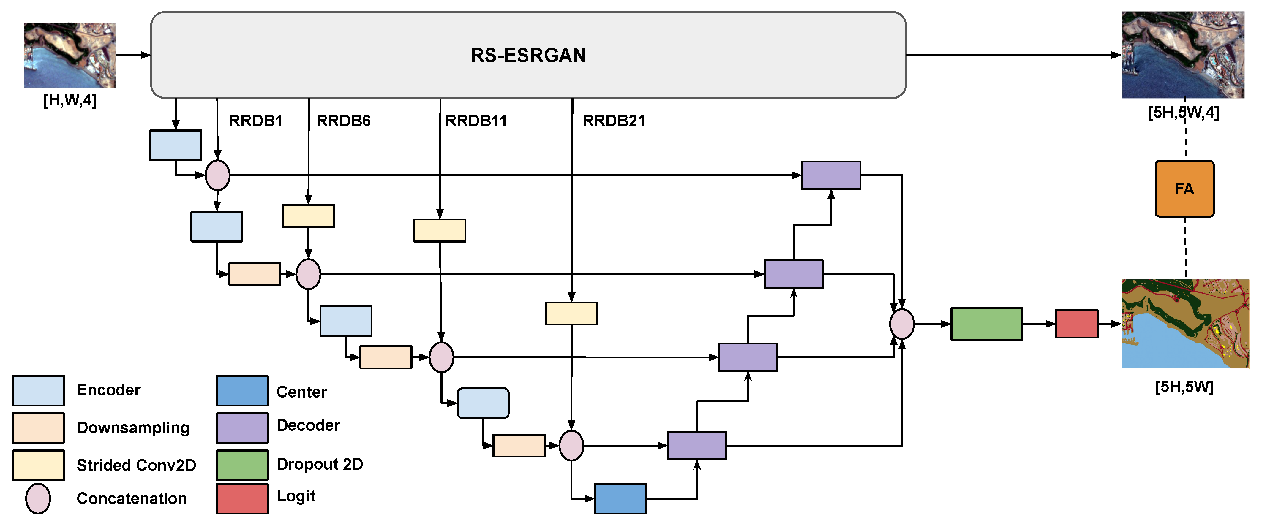
While RS-ESRGAN produces the SR image, several skip connections are retrieved from the feature extraction block of the RS-ESRGAN to reuse some of the features. From the 23 RRDBs in the feature extraction part of RS-ESRGAN, we retrieve output features from the RRDB-1, RRDB-6, RRDB-11 and RRDB-21 blocks, which were determined after hyperparameter tuning. These features are concatenated with outputs of the various sub-blocks of the encoder part, combining knowledge and reinforcing the synergy from both tasks.
The detailed architecture of the SEG-ESRGAN is shown in Figure 6. The encoder is composed of four sub-blocks (Figure 7a), where each encoder sub-block (Enc i in the figure) is a sequence of RRDB, Batch-Normalization (BN) and Spatial and Channel Squeeze and Excitation (scSE) block [85], which is also known as a dual attention block [55] or simple Squeeze and Excitation blocks [56]. The architecture of the scSE block is shown in Figure 7b.
To increase the receptive field and to promote holistic feature information, the output of each encoder sub-block is downsampled. Thus, to match spatial sizes, the features retrieved by the skip connections are processed with a dilated 2D convolution, which is latter concatenated with the respective encoder output, to mix information from the SR and segmentation tasks.
The RRDB block in each encoder sub-block produces relevant feature extraction in a dense manner, concatenating and combining different low-level information to have richer high-level content. Later, output features from the BN are refined by a scSE block, which is composed of a dual-path attention block that focuses on retrieving meaningful characteristics in the spatial and spectral domains. We use the same 2D convolution configuration for the RRDB and scSE blocks (a 3 × 3 kernel and stride of 1) in the encoder’s sub-blocks.
Regarding the architecture of the Squeeze and Excitation blocks (see Figure 7b), in the spatial domain, the input features are multiplied by a weight map w s that recalibrates the focus on relevant spatial content. This weight map is obtained after a 2D convolution operation with a 1 × 1 kernel that squeezes the input channels to 1 and, then, passes through a sigmoid, gathering relevant spatial information from the input features.
Several authors [32,86] have already shown that all channels do not contribute equally to attain the best performance. Therefore, in the channel squeeze and excitation block, a Global Average Pooling (GAP) operates over the input features to produce a single vector with the most relevant value per channel. Then, the information given by the vector is squeezed and expanded by a pair of 1 × 1 2D convolutions [18] with a ratio r equal to four, to reduce the inter-channel correlation and promote the flow of relevant feature content for the next block. Finally, a sigmoid activation produces the weight vector w c that operates over the input feature to find the most relevant spectral content from the features maps.
The first encoder sub-block of Figure 6 processes 64 feature maps from the first convolution of the generator of RS-ESRGAN. The subsequent encoder sub-blocks accept an additional 64 feature maps from the skip connection that are concatenated with the previous encoder block output. Thus, each encoder processes more feature maps and encodes more context in its features.
After passing through the four encoder sub-blocks, the features are downsampled and concatenated with the final skip connection from the RRDBs of the RS-ESRGAN block. The final output stride (the spatial ratio of the downsampled features with respect to their original size) of these high-level features is 16.
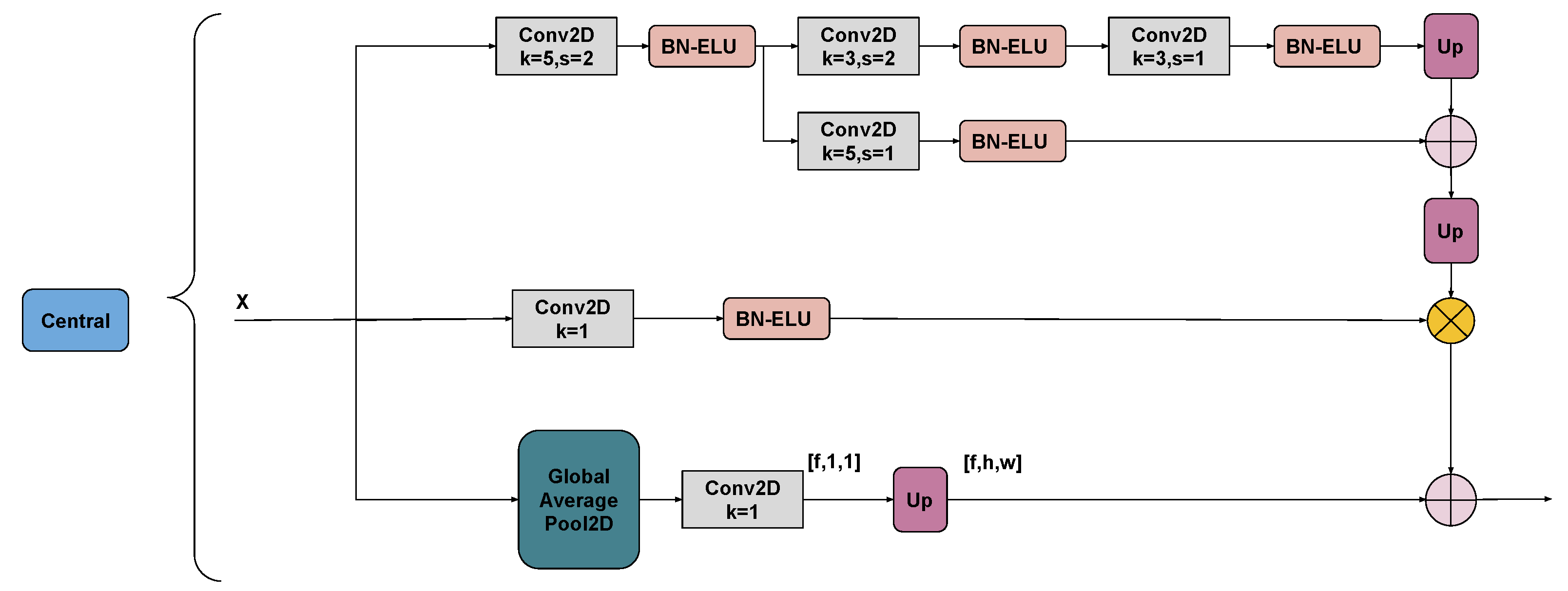
The architecture of the central and decoders sub-blocks was inspired by the work of [87]. The central sub-block is a variant of a Feature Pyramid Attention block [88]. Figure 8 illustrates the architecture that merges information from three different scales, using different kernel sizes, promoting context information retrieval from high-level feature maps.
As in a U-Net, each decoder sub-block combines low with high-level complexity feature content. Figure 9 exhibits its architecture, where an upsampling layer rescales the high-level features that are concatenated with low-level features from the encoder part. Then, a sequence of BN and scSE reinforces highly relevant content for the next decoder block.
All decoders outputs are concatenated, matching sizes with interpolation, to produce a hyper-column [89] of feature maps that enrich the descriptors and information from all different levels of the decoder, and encourage fine-grained segmentation of objects. Finally, according to Figure 6, we add a spatial dropout layer [90] to prevent over-fitting and a logit layer with a 2D convolution to obtain the output channels, which produce one segmentation map per class.
Thus, we present a novel architecture that reuses high-level feature maps from different feature extraction stages of the generator of RS-ESRGAN, richer in high-frequency content, to help in the segmentation capacity of the encoder–decoder network. The segmentation branch is composed of RRDB blocks, which enhance the network capacity and scSE blocks that focus on meaningful content, in this manner producing an SR image and an accurate corresponding segmentation map.

3.3. Loss Functions

Similarly to the works of [6] and [2], we use the same multi-loss approach for training the multi-task network. We use two dedicated losses for each branch and a feature affinity loss for combining the learning of both branches.
Regarding the super-resolution branch, the L1 norm was computed between the intensity pixel values of the SR output Y ^ and the target Y, for images with shape H × W and C channels:
L 1 ( Y ^ , Y ) = 1 C H W k = 1 C j = 1 H i = 1 W | Y ^ i j k Y i j k |
For the semantic segmentation branch, we use the weighted Cross-Entropy loss (CE). For each pixel of the output map, a class vector y i j ^ is predicted with the corresponding scores for each class. Each pixel in the target map y i j is one-hot encoded, containing a 1 for the corresponding class and zero for the rest, K being the number of classes. The loss is averaged over the entire map, with H x W shape, as shown below:
L C E ( y ^ , y ) = 1 H W j = 1 H i = 1 W k = 1 K w k y i j ( k ) l o g ( y i j ^ ( k ) ) ,
The weights for each class w k are computed from the training sub-set of the dataset, using Equation (3), as in [2] and [91], where β k corresponds to the frequency of occurrence of the class, and the term 1.02 is added for stability, in case of β k = 0 .
w k = 1 l n ( 1.02 + β k )
Spatial details are essential for making an accurate segmentation; thus, structural information in the SISR branch can be contrasted with semantic information from the segmentation branch, even though not directly. Therefore, to share the learning between both branches, we use the same implementation of feature affinity loss as explained in [2,6], in which similarity matrices S are calculated from HR feature maps from both branches, looking for strong connections between pixels in the feature domain. The feature affinity loss (Equation (4)) computes the L1 distance between these similarity matrices.
L F A ( S ( S S S R ) , S ( S I S R ) ) = 1 W 2 . H 2 i = 1 W . H j = 1 W . H S i j ( S S S R ) S i j ( S I S R ) ,
where S ( S S S R ) and S ( S I S R ) refer to the SSSR and SISR similarity matrices, respectively.
The final loss we use for training the model consists of a linear combination of the above-mentioned losses, as shown in Equation (5):
L = L C E + w 1 L 1 + w 2 L F A ,
where w 1 and w 2 are hyper-parameters set to make the loss ranges comparable. In our case, we obtained the best weighting w 1 = 1.0 and w 2 = 0.1 .

3.4. Quantitative Metrics

To evaluate the super-resolution performance, we use the traditional PSNR and SSIM, as well as two additional metrics (ERGAS, and SAM) for measuring the spectral quality of the results [7].
  • Peak Signal to Noise Ratio (PSNR) assesses the reconstruction quality of the image, where higher value implies better quality.
  • Structural Similarity (SSIM) [92] compares three features of the image (luminance, contrast and structure). Values close to 1 indicate high matching between the compared images.
  • Erreur relative globale adimensionnelle de systhese (ERGAS) [93] measures the per-channel error between the images considering the scaling factor M, as well. In this case, a lower value indicates a better reconstruction.
  • Spectral Angle Mapper (SAM) [94] provides an indication of the spectral similarity of both images, where lower values means lower spectral distortion.
For the segmentation performance, we use standard metrics such as IoU, confusion matrix, Precision, Recall and F1-score.
  • Intersection-Over-Union (IoU) computed as the ratio between the overlap of the predicted segmentation area and the GT, and the union of these areas. The range of this metric is between 0 (indicating no overlapping) and 1 (indicating full overlap).
  • Confusion matrix is helpful to assess a multi-class classification or segmentation task. The rows of the confusion matrix indicate the true instances of each class, whilst the columns correspond to instances predicted for each particular class.
    The diagonal samples are the True Positive (TP) values for each class, corresponding to the number of samples of the class that are correctly classified.
    There are two different indicators for mis-classification. In False Positive (FP), the sample predicted for a class actually belongs to another class. In False Negative (FN), the sample of a particular class was predicted as belonging to another class. The Intersection over Union for a particular class i ( I o U i ) is:
    I o U i = T P i T P i + F N i + F P i
  • The Precision of class i ( P i ) is the rate of TP i over all predictions for that class, and the Recall ( R i ) measures the ratio of TP i over the GT of that class. Considering the confusion matrix presented above, the metrics for a particular class (C i ) can be computed as follows:
    P i = T P i T P i + F P i R i = T P i T P i + F N i
  • F1-score is the harmonic mean of the Precision and Recall of a particular class, which gives an overall measure considering both metrics:
    F 1 i = 2 P i R i P i + R i

3.5. Training Details

We trained our model using 308 patches of 160 × 160 pixels without overlap, using horizontal and vertical flips, as well as random crops of 160 × 160 pixels for data augmentation, standardizing by channels using the corresponding mean and standard deviation. The model was trained for 200 epochs with early stopping and saving the best weights according to the mIoU metric. After hyperparameter tuning, we used a batch size of 4, a learning rate of 5 × 10 4 with AdamW [95], an improved version of Adam, as optimizer and weight-decay of 5 × 10 5 . Different learning rate schedulers were tested, obtaining the best performance using CosineAnnealing.

4. Results

This section presents the results achieved with our model and a comparison made with other segmentation and multi-task models. Section 4.1 presents the results obtained by performing an inference on the Maspalomas dataset, to select the best weights of the RS-ESRGAN model that were used to initialize the SR branch on the multi-task model. Section 4.2 presents the results of our proposal and in Section 4.3 we provide a comparison with other models that were trained with the Maspalomas dataset. Finally, in Section 4.4 we introduce different inference results with different Sentinel-2/WorldView images, that do not belong to the Maspalomas dataset, to show the generalization ability of our proposal.

4.1. RS-ESRGAN Inference

RS-ESRGAN [7] is a super-resolution network that maximizes its performance by combining network weights achieved after different training stages. First, it trains only the generator, calling this network a PSNR-oriented mode, and then, it fine-tunes this generator with an adversarial training. The best weights for the generator are obtained by interpolation, using Equation (9). By this means, it minimizes the noise–blur trade-off, getting results with more texture and finer details.
G ( X ) = ( 1 α ) G P S N R o r i e n t e d ( X ) + α G a d v ( X ) ,
where G P S N R o r i e n t e d are the best weights achieved after training the generator alone and G a d v are the best weights of the generator after training in an adversarial mode.
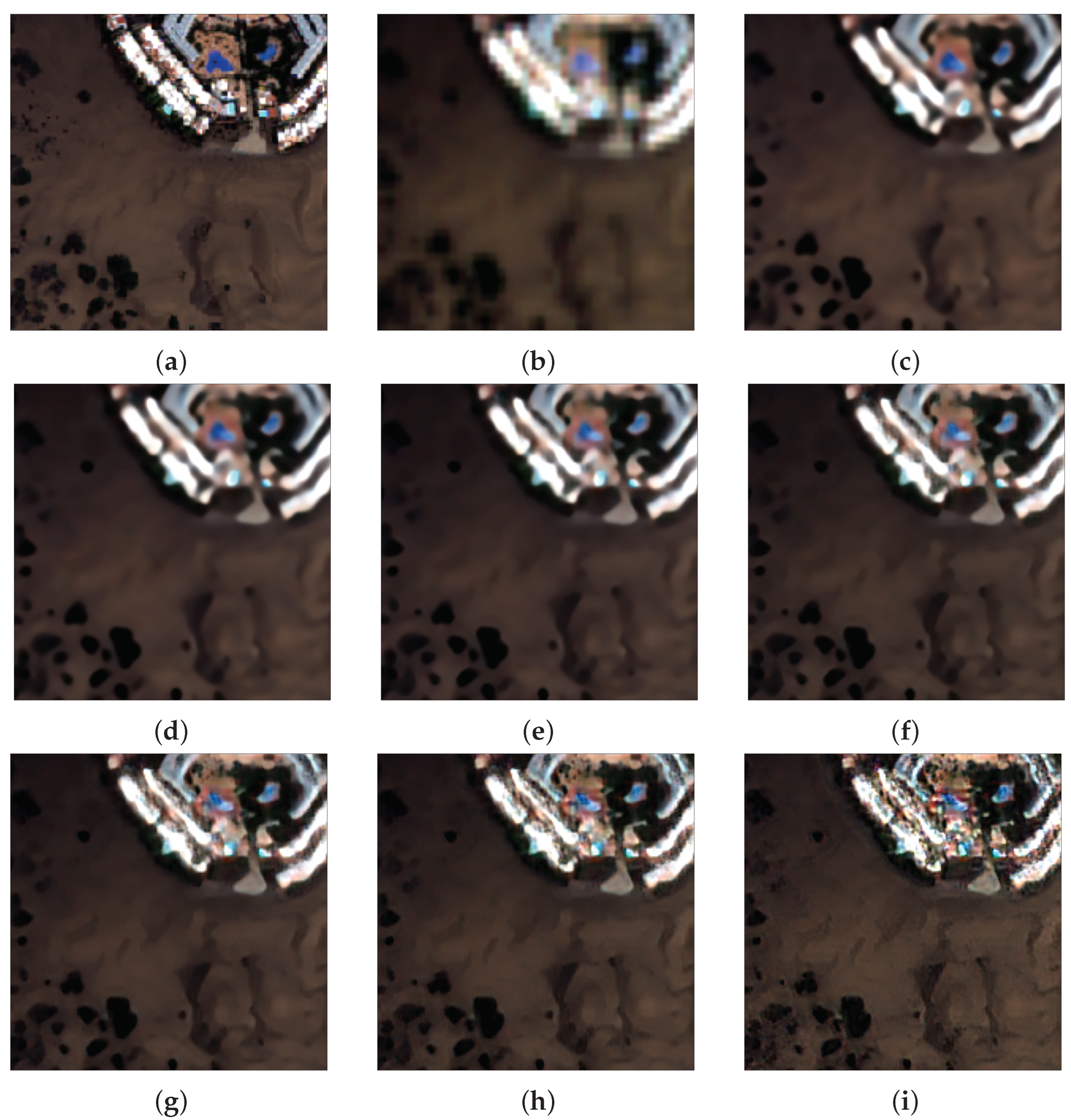
By using the different pre-trained weights of RS-ESRGAN [7], we perform inference on the test set of the dataset to choose the best weights that initialize the SR branch of the multi-task model. We used different values of α in Equation (9) that balance the contribution of a PSNR-oriented model with α = 0 (SR_0), which tends to produce enhanced images but still a little blurry, and a fully adversarial model (SR_ 1.0 ) with α = 1 , which tends to refine texture but introduces noise, as well.
Table 2 shows the mean results according to the PSNR, SSIM, ERGAS and SAM metrics. We can notice that the best result was achieved using α = 0.1 for the PSNR and SSIM metrics, that focus on the reconstruction of higher detailed images. On the other hand, ERGAS and SAM metrics are indicative of the spectral information with respect to the target image.
Figure 10 shows the SR results of this inference on the test set. We can notice a little spectral difference but with a considerable winning margin concerning the delineation of the buildings and the swimming pools in the image. However, if we look carefully at the images with α > 0.5 , we notice some distortion around the edges of objects that hinders the final result.

4.2. SEG-ESRGAN Results

The final architecture of SEG-ESRGAN was achieved after several experiments, as described in Appendix A. We obtained our best results after loading the pre-trained weights for the SR branch (using α = 0.1) and fine-tuning the branch. The rest of the blocks are initialized using the Kaiming method [96].
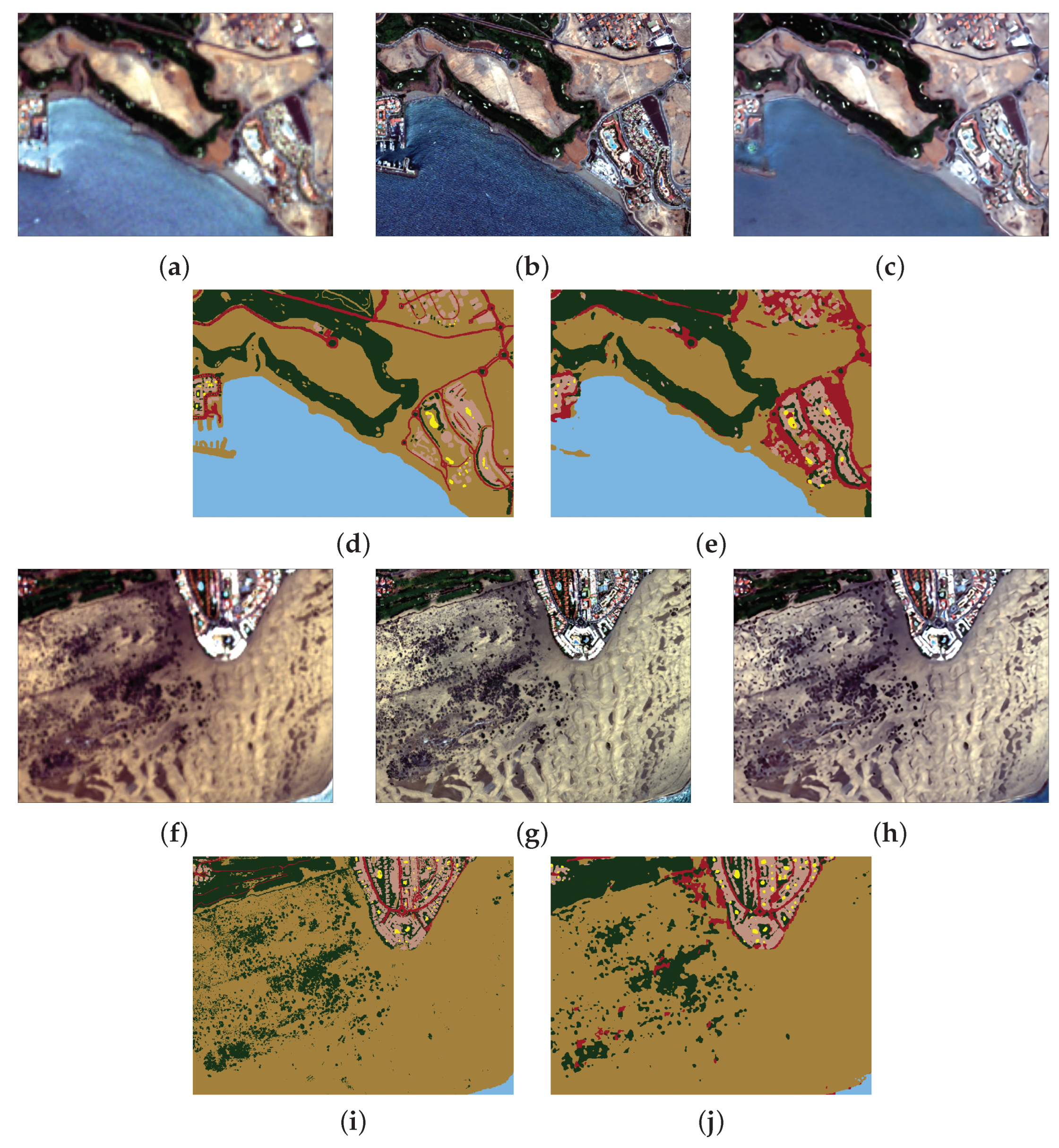
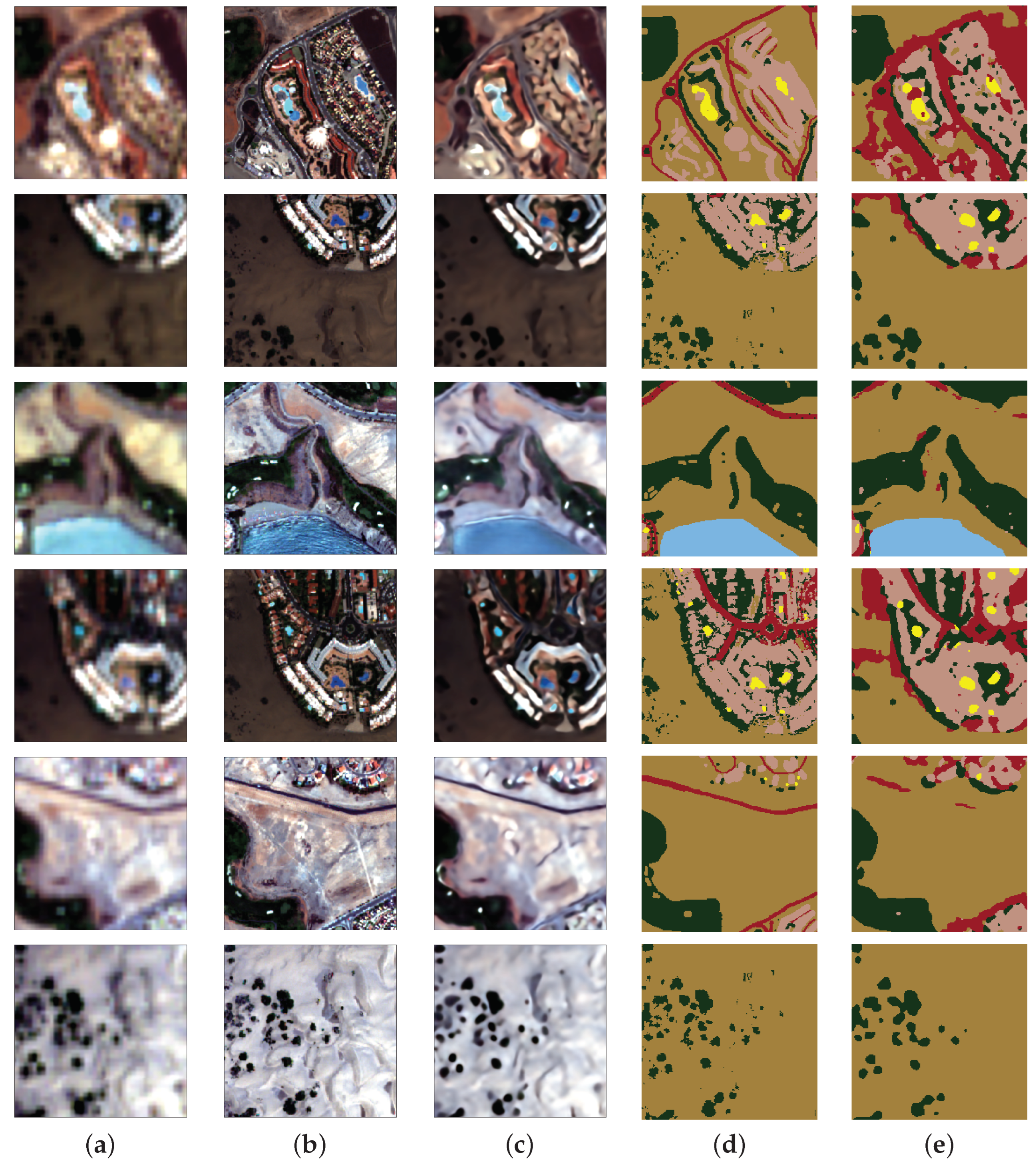
Figure 11 shows the results of our model, with a zoom of some regions in Figure 12. We notice on the predicted map of Figure 11d that areas of bare ground are discernible among the vegetation located in the central part of the image near the water. In the same figure, we can see that the port area could not achieve a continuous segmentation, and the neighborhood in the upper right was recognized to some extent, although it is a challenging area, as it can be seen in the input image in Figure 11a.
Looking at Figure 11i, we can notice that it tends to confuse some areas of vegetation and bare soil with asphalt. Note the complexity of the classification of the original Sentinel-2 image due to the heterogeneity and size of the existing land covers, with narrow roads, small constructions, pools, and dark small shrubs and wet sandy areas over the dunes.
However, we highlight the excellent performance on detecting most of the land covers, specially swimming pools in the residential area. Inspecting the details in the zooming plots of Figure 12, we notice even more the performance on detecting small pools in the second and third rows. It is important to highlight the delineation and clear edges in the SISR results in comparison with the Sentinel-2 input image in the first column at the same figure.
Regarding the quantitative SS performance, Table 3 shows the confusion matrix with extra columns for the precision, F1-score and IoU metrics, as well as the amount of pixels per class in the test set (Total Pixels). The confusion matrix is normalized per rows (recall metric on the diagonal) showing outstanding performance for water and bare soil, which are the majority classes, and around 75% of recall for the other classes, except for the asphalt class. We can appreciate the confusion between asphalt class with bare soil and vegetation. The precision rate for that class only reaches 33% with a recall of 64%. This confusion can be explained because of the high spectral similarity between these classes, especially in the dunes zone and in other areas where the vegetation can be easily confused with dark bare soil. Actually, this fact represented a challenge to manually correct the labeled pixels in the dataset.
Table 4 shows the SR metrics in comparison with the bicubic interpolation. We can see that our model improves regarding the considered metrics; however, if we compare with the results obtained with inference using RS-ESRGAN alone (Section 4.1), our model has lost a little of the SR performance to improve the segmentation results.
Nevertheless, if we visually inspect the zoom results in Figure 12, we can notice the improvements regarding the details in the delineation of roads and buildings as well as in the small vegetation in the dunes zone.

4.3. Comparison with Other Models

To measure the performance achieved by our SEG-ESRGAN, we compared our super-resolution and segmentation results with other state-of-the-art models, such as:
  • U-Net [51] trained with bicubic Sentinel-2 and SR images from RS-ESRGAN as input;
  • DeepLabV3+ [49] trained with bicubic Sentinel-2 images as input;
  • HRNet [54] trained with bicubic Sentinel-2 images as input;
  • Dual_DeepLab [2] trained with bicubic Sentinel-2 images as input,
where the SR images were achieved by using the RS-ESRGAN in inference mode.
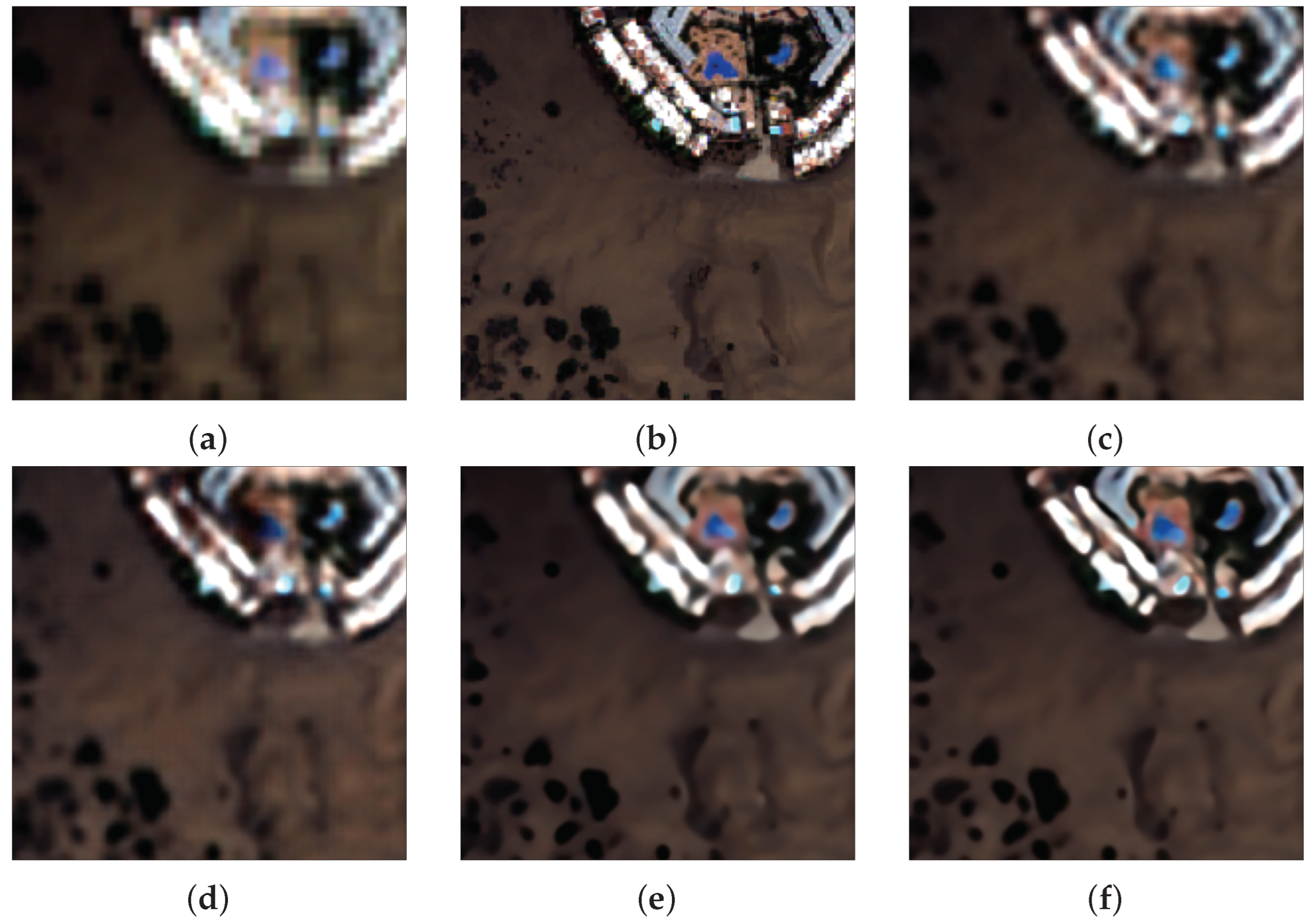
We use the F1-score to measure the performance per class, as it better encompasses the precision and recall, along with the mean IoU, as a global segmentation metric. Table 5 and Table 6 show the segmentation and super-resolution metrics, respectively, while Figure 13 and Figure 14 show several samples of the segmentation and super-resolution results.
Our proposed model outperforms modern fully segmentation methods (U-Net, Deep-
LabV3+ and HRNet) that do not produce an SR image. We also trained a U-Net with ResNet-101 as an encoder, with super-resolved images that were previously inferred using RS-ESRGAN; see Section 4.1. We named this model U-Net+SR, and, in this opportunity, the results improved in comparison with the U-Net that was trained using bicubic interpolated Sentinel-2 images, although still, our proposal has a better performance in almost all the classes.
For the comparison with the Dual_DeepLab model [2], we also trained the model using the same training strategy, but adjusting the architecture to be suitable for the dataset, i.e., we removed the extra-upsampling module from both decoder blocks, as the input is already interpolated to the target spatial resolution. We proposed modifications to the Dual_DeepLab model by adding RRDB blocks with separated convolutions to the decoders sub-block, calling this model Dual_DeepLab_RRDB. This modification increases the generation capacity of the decoder by making more feature maps and boosting the performance on the segmentation part. However, our SEG-ESRGAN proposal still produces better segmentation results in almost all the classes except in the asphalt class.
We also show the results obtained by training a U-Net with ResNet-101 as the encoder, using only WorldView images with the same training strategy. By this mean, we provide an upper bound that can be achieved when training a pure segmentation model with very-high resolution images as input to the network.
Analyzing Table 6, although our model performs a bit worse than RS-ESRGAN with α = 0.1 (U-Net+SR) in terms of some super-resolution metrics (PSNR, SSIM, ERGAS), if we better inspect the samples corresponding to the RS-ESRGAN inference and our SEG-ESRGAN model, in Figure 14, we barely notice the difference between both results.
It is worth analyzing the number of parameters and memory consumption of our proposed model. Table 7 shows the number of trainable parameters of each model and the estimated consumption in memory. We can notice that ESRGAN has 16.6 million parameters and needs 33 MB of memory. Our model, based on RS-ESRGAN, only adds 14.2 million parameters and nearly 28 MB of extra memory to perform the segmentation task. On the other hand, our best competitor (U-Net+SR) needs to use the ESRGAN model to perform SR first and, then, it uses an extra 103 MB to train the 51.5 million parameters of a U-Net with a ResNet-101 encoder.

4.4. Inference on Other Sentinel-2/WorldView Imagery

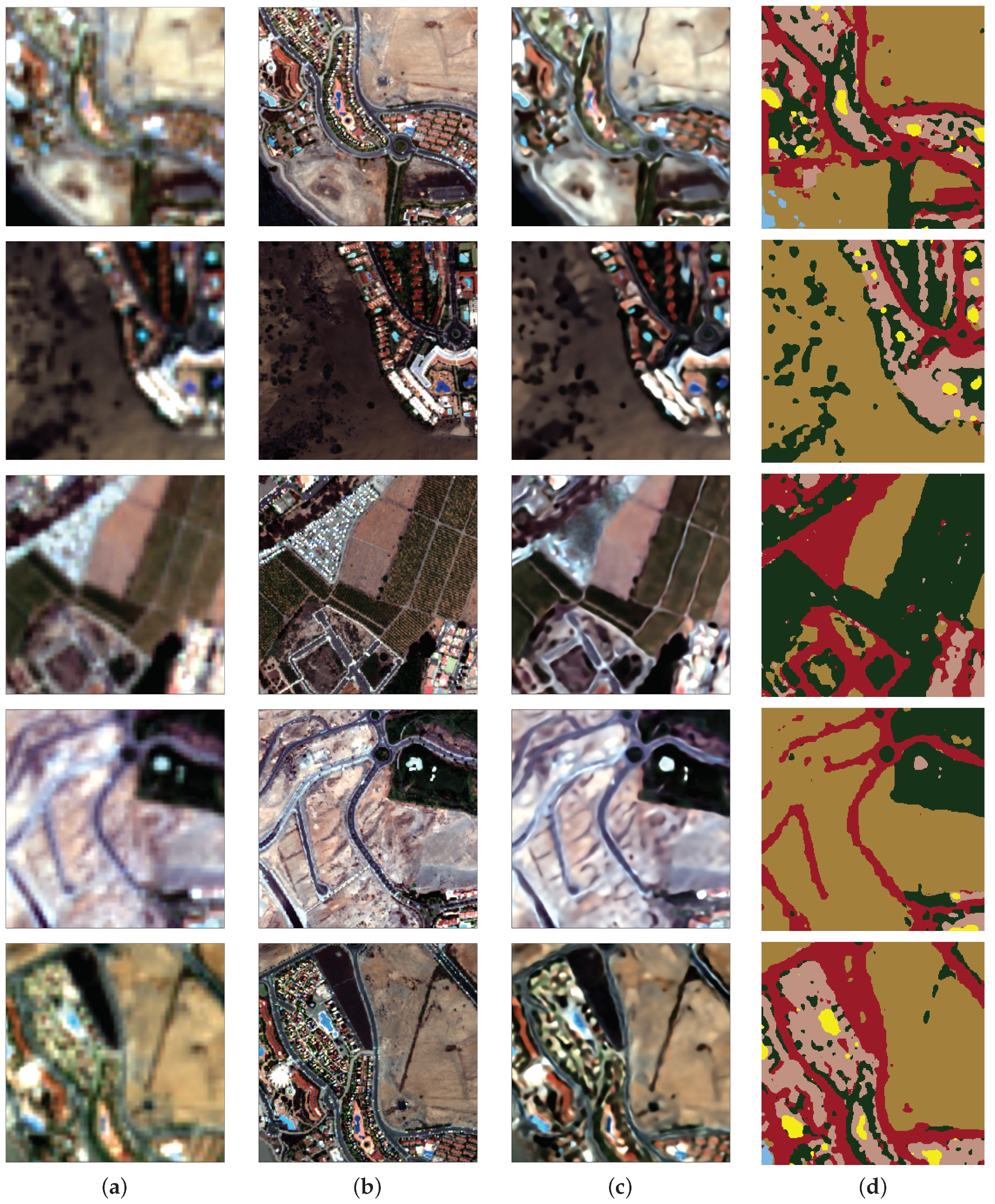
To explore the generalization performance on different image pairs of WorldView-Sentinel, we used the two pairs described in Table 8. Both datasets were preprocessed as described in [7] before any inference and analysis. Figure 15 shows different results in crops extracted from those pairs. We can notice that our SISR predictions are consistent with the GT image as well as with the segmentation predicted.

5. Discussion

One of the main challenges working with deep learning models is to have a suitable dataset for training. In this work, tackling the SR of Sentinel-2 bands, we paired the 10 m bands with the corresponding bands of WorldView-2 at 2 m of spatial resolution, forming a dataset of LR-HR with a scaling factor of 5. We are not aware of other datasets that have also their corresponding land-cover annotations for such high spatial resolution, and, as already shown in [2], the authors also rely on released land-cover maps that may often represent a class mismatch between the input and the corresponding GT. Therefore, to work with a high scaling factor, we opted for manually correcting an SVM map, generated with few annotations, even being time-consuming.
One of the main limitations when producing a multisensor dataset is the difficulty to guarantee the same information. Specifically, although we are using images from different sources taken on the same day, there are still spectral differences between them. Even applying the proper radiometric calibrations, advanced atmospheric correction models and co-registration to assure the geographic matching of pixels, these differences are mainly due to different shadows caused by differences in the acquisition time and off-nadir viewing angles or radiometric variations that are difficult to get rid off.
Concerning our final SEG-ESRGAN model, it was obtained after loading pre-trained weights on the super-resolution branch and letting the network adjust them. This model achieved the best performance regarding the segmentation task and without losing details in the SISR image. The proposed architecture included an encoder with sub-blocks of RRDB-BN-scSE, achieving excellent segmentation results, even in a class with few annotations (swimming pools), as it can be seen in Table 3. This can be attributed to the great capacity and higher performance showed by RRDB blocks in generating richer features, which are also benefited from the dense connections. After the features were processed by the RRDB and the BN in the encoder sub-block, scSE takes these features and dynamically determines the best spatial and spectral characteristic to be transferred to the next encoder sub-block.
We demonstrated that super-resolution and segmentation networks can work together using skip connections to retrieve high-level features with high resolution that can yield better segmentation performance. Even in a challenging scenario, having considerable similarity between classes, our model can produce consistent segmentation as well as detailed edges in the super-resolved image, as shown in the zoom images in Figure 12.
Regarding the SR performance, our model was compared to a bicubic interpolation and with the Dual_DeepLab model [2], obtaining better quantitative metrics and qualitative enhancements, as shown also in Figure 12 and in Table 6. We also proposed a variant to the Dual_DeepLab architecture to increment the dense connections by adding RRDBs in both decoders.
Regarding the segmentation performance, we compared our model with other full segmentation networks such as U-Net, DeepLabV3+ and HRNet, as well as with Dual_DeepLab and its variant, the Dual_DeepLab_RRDB. All these experiments were completed using the bicubic interpolated Sentinel-2 as input. Table 5 shows that our model achieves 0.74 in mean F1 and 0.6278 in mean IoU, having a good approximation to the upper bound performance, which was achieved with a U-Net (ResNet-101 as encoder) with only HR WorldView-2 images (mF1 = 0.7883 and mIoU = 0.6723). In addition, we used the pre-trained weights of RS-ESRGAN [7] in inference mode to produce an SR version of the Maspalomas dataset. With these enhanced images, we trained a U-Net model with ResNet-101 as an encoder to produce an SSSR label map. Our model reduces its performance on the SR task to achieve a better result in segmentation. Note that we did not make a comparison regarding the native resolution of Sentinel-2 bands, mainly because we lack the corresponding GT labels at that resolution and, as it has already been proved in [2] and [76], a multi-task network tends to perform better with spatial enhanced images.
It is important to highlight that the spatial resolution has been increased by a challenging factor of 5. That is, the original 100 m 2 pixel area has been enhanced to 4 m 2 . Note that small objects or covers do not appear in the original Sentinel-2 image and are intended to be shown in the final segmentation map. Nevertheless, the land cover maps achieved are quite similar to the ground truth obtained with WorldView-2 data. Specifically, the model performs well in discriminating small swimming pools in residential areas. This can be of interest for city councils, as the possibility of using free medium-resolution images can reduce the budget and effort of monitoring large areas, but we are aware that this topic needs further investigation.
Finally, we indicate that our model significantly reduces memory consumption and the number of parameters to achieve excellent performance regarding segmentation and super-resolution tasks.

6. Conclusions

The main objective of this work was to use the Sentinel-2 bands in applications that require high resolution, and by this mean, avoiding the high cost required in the acquisition of very-high resolution imagery, especially in studies involving great surface coverage of multitemporal analysis.
In this context, we propose an encoder–decoder network architecture that obtains high-resolution segmentation maps along with a super-resolved image, with a factor of 5, from a low-resolution multispectral Sentinel-2 imagery. To produce the SR image, we based our model on an RS-ESRGAN and retrieve skip connections that are used to produce the final segmentation map.
We develop a novel dataset consisting of registered WorldView/Sentinel-2 pairs for the region of Maspalomas, Canarias-Spain and the corresponding segmentation map using the WorldView-2 image. We manually labeled and corrected the land-cover maps produced using an SVM classifier to reduce the noise and mis-labeling errors.
Our model, named SEG-ESRGAN, achieved a global mean F1 = 0.74 and a weighted F1 = 0.8783, as well as an mIoU = 0.6278 regarding the segmentation task. If we compare these values with a baseline U-Net using a bicubic 2 m Sentinel-2 as input (mF1 = 0.7133, wF1 = 0.8677, and mIoU=0.5904), our model outperforms by a good margin. Even using the same U-Net model with improved SR images (mF1 = 0.7233, wF1 = 0.8651, and mIoU=0.6003), our model still performs better and approaches very well to the performance achieved with a U-Net trained with only WorldView-2 images (mF1 = 0.7883, wF1 = 0.8944 and mIou = 0.6723).
Considering the SR performance, our model provides enhanced images with better spatial detail and minimum spectral distortion. It achieved a PSNR = 30.786 and SSIM = 0.816 that outperforms the baseline bicubic interpolation (PSNR = 29.452 and SSIM = 0.792). In addition, we tested SEG-ESRGAN on a different set of Sentinel-2 and WorldView imagery not belonging to the train–test subsets, obtaining excellent results as well.
Furthermore, for generating the extra SSSR map, our model only adds 14.2 M parameters and 28 MB to the already proposed RS-ESRGAN, making these small extra features reach better segmentation results than other state-of-the-art models.

Author Contributions

Conceptualization, L.S., J.M. and V.V.; data curation, L.S.; methodology, L.S., J.M. and V.V.; software, L.S.; supervision J.M. and V.V.; validation, L.S., J.M. and V.V.; formal analysis, L.S., J.M. and V.V.; resources, L.S., J.M. and V.V.; writing—original draft preparation, L.S., J.M. and V.V.; writing—review and editing, L.S., J.M. and V.V.; funding acquisition, L.S., J.M. and V.V. All authors have read and agreed to the published version of the manuscript.

Funding

This work was funded by the Spanish Agencia Estatal de Investigación (AEI) under projects ARTEMISAT-2 (CTM 2016-77733-R), PID2020-117142GB-I00 and PID2020-116907RB-I00 (MCIN/AEI call 10.13039/501100011033). L.S. would like to acknowledge the BECAL (Becas Carlos Antonio López) scholarship for the financial support.

Data Availability Statement

Sentinel-2 data can be downloaded from https://scihub.copernicus.eu/dhus/#/home (accessed on 7 October 2022). Restrictions apply to WorldView-2 data due to single user license applies.

Conflicts of Interest

The authors declare no conflict of interest.

Abbreviations

The following abbreviations are used in this manuscript:
ASPPAtrous Spatial Pyramid Pooling
BNBatch Normalization
CECross-Entropy
CNNConvolutional Neural Network
DLDeep Learning
ERGASErreur relative globale adimensionnelle de systhese
FAFeature Affinity
GANGenerative Adversarial Network
GAPGlobal Average Pooling
GTGround-Truth
HRHigh Resolution
IoUIntersection over Union
LRLow Resolution
LULCLand Use and Land Cover
MSMultispectral
NIRNear Infrared Band
PSNRPeak Signal-to-Noise Ratio
RRDBResidual-in-Residual Dense Block
RSRemote Sensing
SAMSpectral Angle Mapper
scSESpatial and Channel Squeeze and Excitation
SEG-ESRGANSegmentation Enhanced Super-Resolution GAN
SISRSingle Image Super-Resolution
SRSuper-Resolution
SSSemantic Segmentation
SSIMStructural Similarity Index Measure
SSSRSemantic Segmentation Super-Resolution
SVMSupport Vector Machine

Appendix A. SEG-ESRGAN Model Architecture

We performed several experiments to define our best model architecture. Table A1 summarizes the different versions tested and Table A2 shows the corresponding performance using F1-score metric. Although minor changes were made between each version, we present the main variations between each architecture besides the training details, as follows:
  • v1: We based our model using the RS-ESRGAN as the trunk for the dual network. From the feature extraction module of RS-ESRGAN, composed of sequential RRDB blocks, we retrieved four skip connections at different levels. These features are downsampled to different scales to emulate the UNet architecture and to extract context. Then, the features are connected to the decoder to produce the final segmentation map. These blocks are maintained in almost all the versions, as depicted in our best proposal in Figure 6.
  • v2: We used the blocks of Resnet-101 as encoder. The first feature map is retrieved with a skip-connection from the shallow feature extraction block of the RS-ESRGAN. We noticed that using the Resnet blocks increased the memory consumption of the dual network.
  • v3: We used scSE blocks as encoders. These blocks do not consume much memory and have good performance, obtaining useful features that are concatenated with the skip connections from the ESRGAN.
  • v4: We added RRDB modules and BN along with scSE to form the encoder blocks. We trained the entire network from scratch without loading any pre-trained weights to the RS-ESRGAN trunk.
We achieved our best results initializing the SR branch with the pre-trained weights of the RS-ESRGAN network and conducting a hyper-parameter sweep over model v4 using WandB [97]. We searched over the batch size, the learning rate, loss weights in Equation (5), and different levels for the skip connections from the RS-ESRGAN.
Table A1. Different versions of the SEG-ESRGAN architecture.
Architecturev1v2v3v4
- Skip connections as encoderxxxx
- Encoder ResNet-101 x
- Encoder scSE xx
- Encoder RRDB + scSE x
Analyzing Table A2, we notice that using the combination of RRDB-BN-scSE in each encoder block produced an increment of the performance in the minority class (the swimming pool) that motivated us to continue with this architecture.
Table A2. Different versions of the SEG-ESRGAN model and the performance on each class using the F1 metric. Best values in bold.
WaterVegetationPoolBare SoilAsphaltBuilt SoilMean F1
SEG-ESRGAN_v10.950.740.460.910.500.640.702
SEG-ESRGAN_v20.950.780.580.910.320.610.692
SEG-ESRGAN_v30.960.770.510.920.440.670.710
SEG-ESRGAN_v40.970.730.590.920.420.680.719

References

  1. Ma, L.; Liu, Y.; Zhang, X.; Ye, Y.; Yin, G.; Johnson, B.A. Deep learning in remote sensing applications: A meta-analysis and review. ISPRS J. Photogramm. Remote Sens. 2019, 152, 166–177. [Google Scholar] [CrossRef]
  2. Abadal, S.; Salgueiro, L.; Marcello, J.; Vilaplana, V. A Dual Network for Super-Resolution and Semantic Segmentation of Sentinel-2 Imagery. Remote Sens. 2021, 13, 4547. [Google Scholar] [CrossRef]
  3. Alparone, L.; Aiazzi, B.; Baronti, S.; Garzelli, A. Remote Sensing Image Fusion; Crc Press: Boca Raton, FL, USA, 2015. [Google Scholar]
  4. Minaee, S.; Boykov, Y.Y.; Porikli, F.; Plaza, A.J.; Kehtarnavaz, N.; Terzopoulos, D. Image segmentation using deep learning: A survey. IEEE Trans. Pattern Anal. Mach. Intell. 2021. [Google Scholar] [CrossRef] [PubMed]
  5. Aakerberg, A.; Johansen, A.S.; Nasrollahi, K.; Moeslund, T.B. Single-loss multi-task learning for improving semantic segmentation using super-resolution. In Proceedings of the International Conference on Computer Analysis of Images and Patterns, Virtual Event, 28–30 September 2021; Springer: Cham, Switzerland, 2021; pp. 403–411. [Google Scholar]
  6. Wang, L.; Li, D.; Zhu, Y.; Tian, L.; Shan, Y. Dual super-resolution learning for semantic segmentation. In Proceedings of the IEEE/CVF Conference on Computer Vision and Pattern Recognition, Seattle, WA, USA, 14–19 June 2020; pp. 3774–3783. [Google Scholar]
  7. Salgueiro Romero, L.; Marcello, J.; Vilaplana, V. Super-resolution of sentinel-2 imagery using generative adversarial networks. Remote Sens. 2020, 12, 2424. [Google Scholar] [CrossRef]
  8. Ledig, C.; Theis, L.; Huszár, F.; Caballero, J.; Cunningham, A.; Acosta, A.; Aitken, A.; Tejani, A.; Totz, J.; Wang, Z.; et al. Photo-realistic single image super-resolution using a generative adversarial network. In Proceedings of the IEEE Conference on Computer Vision and Pattern Recognition, Honolulu, HI, USA, 21–26 July 2017; pp. 4681–4690. [Google Scholar]
  9. Anwar, S.; Khan, S.; Barnes, N. A deep journey into super-resolution: A survey. ACM Comput. Surv. (CSUR) 2020, 53, 1–34. [Google Scholar] [CrossRef]
  10. Wang, Z.; Chen, J.; Hoi, S.C. Deep learning for image super-resolution: A survey. IEEE Trans. Pattern Anal. Mach. Intell. 2020, 43, 3365–3387. [Google Scholar] [CrossRef] [Green Version]
  11. Dong, C.; Loy, C.C.; He, K.; Tang, X. Learning a deep convolutional network for image super-resolution. In Proceedings of the European Conference on Computer Vision, Zurich, Switzerland, 6–12 September 2014; Springer: Cham, Switzerland, 2014; pp. 184–199. [Google Scholar]
  12. Kim, J.; Lee, J.K.; Lee, K.M. Accurate image super-resolution using very deep convolutional networks. In Proceedings of the IEEE Conference on Computer Vision and Pattern Recognition, Las Vegas, NV, USA, 27–30 June 2016; pp. 1646–1654. [Google Scholar]
  13. Lim, B.; Son, S.; Kim, H.; Nah, S.; Mu Lee, K. Enhanced deep residual networks for single image super-resolution. In Proceedings of the IEEE Conference on Computer Vision and Pattern Recognition Workshops, Honolulu, HI, USA, 21–26 July 2017; pp. 136–144. [Google Scholar]
  14. Tong, T.; Li, G.; Liu, X.; Gao, Q. Image super-resolution using dense skip connections. In Proceedings of the IEEE International Conference on Computer Vision, Venice, Italy, 22–29 October 2017; pp. 4799–4807. [Google Scholar]
  15. Dong, C.; Loy, C.C.; Tang, X. Accelerating the super-resolution convolutional neural network. In Proceedings of the European Conference on Computer Vision, Amsterdam, The Netherlands, 11–14 October 2016; Springer: Rotterdam, The Netherlands, 2016; pp. 391–407. [Google Scholar]
  16. Shi, W.; Caballero, J.; Huszár, F.; Totz, J.; Aitken, A.P.; Bishop, R.; Rueckert, D.; Wang, Z. Real-time single image and video super-resolution using an efficient sub-pixel convolutional neural network. In Proceedings of the IEEE conference on computer vision and pattern recognition, Las Vegas, NV, USA, 27–30 June 2016; pp. 1874–1883. [Google Scholar]
  17. Zhang, Y.; Li, K.; Li, K.; Wang, L.; Zhong, B.; Fu, Y. Image super-resolution using very deep residual channel attention networks. In Proceedings of the European Conference on Computer Vision (ECCV), Munich, Germany, 8–14 September 2018; pp. 286–301. [Google Scholar]
  18. Hu, J.; Shen, L.; Sun, G. Squeeze-and-excitation networks. In Proceedings of the IEEE Conference on Computer Vision and Pattern Recognition, Salt Lake City, UT, USA, 18–22 June 2018; pp. 7132–7141. [Google Scholar]
  19. Goodfellow, I.J.; Pouget-Abadie, J.; Mirza, M.; Xu, B.; Warde-Farley, D.; Ozair, S.; Courville, A.; Bengio, Y. Generative adversarial networks. arXiv 2014, arXiv:1406.2661. [Google Scholar] [CrossRef]
  20. Wang, X.; Yu, K.; Wu, S.; Gu, J.; Liu, Y.; Dong, C.; Qiao, Y.; Change Loy, C. Esrgan: Enhanced super-resolution generative adversarial networks. In Proceedings of the European Conference on Computer Vision (ECCV) Workshops, Munich, Germany, 8–14 September 2018. [Google Scholar]
  21. Tsagkatakis, G.; Aidini, A.; Fotiadou, K.; Giannopoulos, M.; Pentari, A.; Tsakalides, P. Survey of Deep-Learning Approaches for Remote Sensing Observation Enhancement. Sensors 2019, 19, 3929. [Google Scholar] [CrossRef] [Green Version]
  22. Garzelli, A. A review of image fusion algorithms based on the super-resolution paradigm. Remote Sens. 2016, 8, 797. [Google Scholar] [CrossRef] [Green Version]
  23. Ma, W.; Pan, Z.; Guo, J.; Lei, B. Super-resolution of remote sensing images based on transferred generative adversarial network. In Proceedings of the IGARSS 2018-2018 IEEE International Geoscience and Remote Sensing Symposium, Valencia, Spain, 22–27 July 2018; pp. 1148–1151. [Google Scholar]
  24. Wald, L.; Ranchin, T.; Mangolini, M. Fusion of satellite images of different spatial resolutions: Assessing the quality of resulting images. Photogramm. Eng. Remote Sens. 1997, 63, 691–699. [Google Scholar]
  25. Lei, S.; Shi, Z.; Zou, Z. Super-resolution for remote sensing images via local–global combined network. IEEE Geosci. Remote Sens. Lett. 2017, 14, 1243–1247. [Google Scholar] [CrossRef]
  26. Haut, J.M.; Fernandez-Beltran, R.; Paoletti, M.E.; Plaza, J.; Plaza, A. Remote Sensing Image Superresolution Using Deep Residual Channel Attention. IEEE Trans. Geosci. Remote Sens. 2019, 57, 9277–9289. [Google Scholar] [CrossRef]
  27. Salgueiro Romero, L.; Marcello, J.; Vilaplana, V. Comparative study of upsampling methods for super-resolution in remote sensing. In Proceedings of the In Proceedings of the Twelfth International Conference on Machine Vision (ICMV 2019), Amsterdam, The Netherlands, 25–28 September 2019; pp. 417–424.
  28. Xu, Y.; Luo, W.; Hu, A.; Xie, Z.; Xie, X.; Tao, L. TE-SAGAN: An Improved Generative Adversarial Network for Remote Sensing Super-Resolution Images. Remote Sens. 2022, 14, 2425. [Google Scholar] [CrossRef]
  29. Pouliot, D.; Latifovic, R.; Pasher, J.; Duffe, J. Landsat super-resolution enhancement using convolution neural networks and Sentinel-2 for training. Remote Sens. 2018, 10, 394. [Google Scholar] [CrossRef] [Green Version]
  30. Teo, T.A.; Fu, Y.J. Spatiotemporal fusion of formosat-2 and landsat-8 satellite images: A comparison of “super resolution-then-blend” and “blend-then-super resolution” approaches. Remote Sens. 2021, 13, 606. [Google Scholar] [CrossRef]
  31. Lanaras, C.; Bioucas-Dias, J.; Galliani, S.; Baltsavias, E.; Schindler, K. Super-resolution of Sentinel-2 images: Learning a globally applicable deep neural network. ISPRS J. Photogramm. Remote Sens. 2018, 146, 305–319. [Google Scholar] [CrossRef] [Green Version]
  32. Zhang, R.; Cavallaro, G.; Jitsev, J. Super-Resolution of Large Volumes of Sentinel-2 Images with High Performance Distributed Deep Learning. In Proceedings of the IGARSS 2020-2020 IEEE International Geoscience and Remote Sensing Symposium, Waikoloa, HI, USA, 26 September–2 October 2020; pp. 617–620. [Google Scholar]
  33. Salgueiro, L.; Marcello, J.; Vilaplana, V. Single-Image Super-Resolution of Sentinel-2 Low Resolution Bands with Residual Dense Convolutional Neural Networks. Remote Sens. 2021, 13, 5007. [Google Scholar] [CrossRef]
  34. Galar, M.; Sesma, R.; Ayala, C.; Albizua, L.; Aranda, C. Learning Super-Resolution for SENTINEL-2 Images with Real Ground Truth Data from a Reference Satellite. ISPRS Ann. Photogramm. Remote Sens. Spat. Inf. Sci. 2020, 1, 9–16. [Google Scholar] [CrossRef]
  35. Panagiotopoulou, A.; Grammatikopoulos, L.; Kalousi, G.; Charou, E. Sentinel-2 and SPOT-7 Images in Machine Learning Frameworks for Super-Resolution. In Proceedings of the International Conference on Pattern Recognition, Online, 10–15 January 2021; Springer: Berlin/Heidelberg, Germany, 2021; pp. 462–476. [Google Scholar]
  36. Beaulieu, M.; Foucher, S.; Haberman, D.; Stewart, C. Deep Image-To-Image Transfer Applied to Resolution Enhancement of Sentinel-2 Images. In Proceedings of the IGARSS 2018-2018 IEEE International Geoscience and Remote Sensing Symposium, Valencia, Spain, 22–27 July 2018; pp. 2611–2614. [Google Scholar]
  37. Everingham, M.; Eslami, S.; Van Gool, L.; Williams, C.K.; Winn, J.; Zisserman, A. The pascal visual object classes challenge: A retrospective. Int. J. Comput. Vis. 2015, 111, 98–136. [Google Scholar] [CrossRef]
  38. Mottaghi, R.; Chen, X.; Liu, X.; Cho, N.G.; Lee, S.W.; Fidler, S.; Urtasun, R.; Yuille, A. The role of context for object detection and semantic segmentation in the wild. In Proceedings of the IEEE Conference on Computer Vision and Pattern Recognition, Columbus, OH, USA, 23–28 June 2014; pp. 891–898. [Google Scholar]
  39. Long, J.; Shelhamer, E.; Darrell, T. Fully convolutional networks for semantic segmentation. In Proceedings of the IEEE conference on computer vision and pattern recognition, Boston, MA, USA, 7–12 June 2015; pp. 3431–3440. [Google Scholar]
  40. Zhu, H.; Meng, F.; Cai, J.; Lu, S. Beyond pixels: A comprehensive survey from bottom-up to semantic image segmentation and cosegmentation. J. Vis. Commun. Image Represent. 2016, 34, 12–27. [Google Scholar] [CrossRef] [Green Version]
  41. Hao, S.; Zhou, Y.; Guo, Y. A brief survey on semantic segmentation with deep learning. Neurocomputing 2020, 406, 302–321. [Google Scholar] [CrossRef]
  42. Lucchi, A.; Li, Y.; Boix, X.; Smith, K.; Fua, P. Are spatial and global constraints really necessary for segmentation? In Proceedings of the 2011 International Conference on Computer Vision, Barcelona, Spain, 6–13 November 2011; pp. 9–16. [Google Scholar]
  43. Garcia-Garcia, A.; Orts-Escolano, S.; Oprea, S.; Villena-Martinez, V.; Martinez-Gonzalez, P.; Garcia-Rodriguez, J. A survey on deep learning techniques for image and video semantic segmentation. Appl. Soft Comput. 2018, 70, 41–65. [Google Scholar] [CrossRef]
  44. Chen, L.C.; Papandreou, G.; Kokkinos, I.; Murphy, K.; Yuille, A.L. Semantic image segmentation with deep convolutional nets and fully connected crfs. arXiv 2014, arXiv:1412.7062. [Google Scholar]
  45. Sultana, F.; Sufian, A.; Dutta, P. Evolution of image segmentation using deep convolutional neural network: A survey. Knowl.-Based Syst. 2020, 201, 106062. [Google Scholar] [CrossRef]
  46. Chen, L.C.; Papandreou, G.; Kokkinos, I.; Murphy, K.; Yuille, A.L. Deeplab: Semantic image segmentation with deep convolutional nets, atrous convolution, and fully connected crfs. IEEE Trans. Pattern Anal. Mach. Intell. 2017, 40, 834–848. [Google Scholar] [CrossRef] [PubMed] [Green Version]
  47. He, K.; Zhang, X.; Ren, S.; Sun, J. Spatial Pyramid Pooling in Deep Convolutional Networks for Visual Recognition. IEEE Trans. Pattern Anal. Mach. Intell. 2015, 37, 9. [Google Scholar] [CrossRef] [Green Version]
  48. Chen, L.C.; Papandreou, G.; Schroff, F.; Adam, H. Rethinking atrous convolution for semantic image segmentation. arXiv 2017, arXiv:1706.05587. [Google Scholar]
  49. Chen, L.C.; Zhu, Y.; Papandreou, G.; Schroff, F.; Adam, H. Encoder-decoder with atrous separable convolution for semantic image segmentation. In Proceedings of the European Conference on Computer Vision (ECCV), Munich, Germany, 8–14 September 2018; pp. 801–818. [Google Scholar]
  50. Badrinarayanan, V.; Kendall, A.; Cipolla, R. Segnet: A deep convolutional encoder-decoder architecture for image segmentation. IEEE Trans. Pattern Anal. Mach. Intell. 2017, 39, 12. [Google Scholar] [CrossRef]
  51. Ronneberger, O.; Fischer, P.; Brox, T. U-net: Convolutional networks for biomedical image segmentation. In Proceedings of the International Conference on Medical Image Computing and Computer-Assisted Intervention, Munich, Germany, 5–9 October 2015; Springer: Cham, Switzerland, 2015; pp. 234–241. [Google Scholar]
  52. Diakogiannis, F.I.; Waldner, F.; Caccetta, P.; Wu, C. ResUNet-a: A deep learning framework for semantic segmentation of remotely sensed data. ISPRS J. Photogramm. Remote Sens. 2020, 162, 94–114. [Google Scholar] [CrossRef] [Green Version]
  53. Iglovikov, V.; Shvets, A. Ternausnet: U-net with vgg11 encoder pre-trained on imagenet for image segmentation. arXiv 2018, arXiv:1801.05746. [Google Scholar]
  54. Wang, J.; Sun, K.; Cheng, T.; Jiang, B.; Deng, C.; Zhao, Y.; Liu, D.; Mu, Y.; Tan, M.; Wang, X.; et al. Deep high-resolution representation learning for visual recognition. IEEE Trans. Pattern Anal. Mach. Intell. 2020, 43, 3349–3364. [Google Scholar] [CrossRef] [Green Version]
  55. Liu, R.; Tao, F.; Liu, X.; Na, J.; Leng, H.; Wu, J.; Zhou, T. RAANet: A Residual ASPP with Attention Framework for Semantic Segmentation of High-Resolution Remote Sensing Images. Remote Sens. 2022, 14, 3109. [Google Scholar] [CrossRef]
  56. Zhang, X.; Li, L.; Di, D.; Wang, J.; Chen, G.; Jing, W.; Emam, M. SERNet: Squeeze and Excitation Residual Network for Semantic Segmentation of High-Resolution Remote Sensing Images. Remote Sens. 2022, 14, 4770. [Google Scholar] [CrossRef]
  57. Zheng, Z.; Hu, Y.; Qiao, Y.; Hu, X.; Huang, Y. Real-Time Detection of Winter Jujubes Based on Improved YOLOX-Nano Network. Remote Sens. 2022, 14, 4833. [Google Scholar] [CrossRef]
  58. Chen, L.C.; Yang, Y.; Wang, J.; Xu, W.; Yuille, A.L. Attention to scale: Scale-aware semantic image segmentation. In Proceedings of the IEEE conference on computer vision and pattern recognition, Las Vegas, NV, USA, 27–30 June 2016; pp. 3640–3649. [Google Scholar]
  59. Sheykhmousa, M.; Mahdianpari, M.; Ghanbari, H.; Mohammadimanesh, F.; Ghamisi, P.; Homayouni, S. Support Vector Machine vs. Random Forest for Remote Sensing Image Classification: A Meta-analysis and systematic review. IEEE J. Sel. Top. Appl. Earth Obs. Remote Sens. 2020, 13, 6308–6325. [Google Scholar] [CrossRef]
  60. Maulik, U.; Chakraborty, D. Remote Sensing Image Classification: A survey of support-vector-machine-based advanced techniques. IEEE Geosci. Remote Sens. Mag. 2017, 5, 33–52. [Google Scholar] [CrossRef]
  61. Marcello, J.; Eugenio, F.; Gonzalo-Martín, C.; Rodriguez-Esparragon, D.; Marqués, F. Advanced Processing of Multiplatform Remote Sensing Imagery for the Monitoring of Coastal and Mountain Ecosystems. IEEE Access 2020, 9, 6536–6549. [Google Scholar] [CrossRef]
  62. Parente, L.; Taquary, E.; Silva, A.P.; Souza, C.; Ferreira, L. Next Generation Mapping: Combining Deep Learning, Cloud Computing, and Big Remote Sensing Data. Remote Sens. 2019, 11, 2881. [Google Scholar] [CrossRef] [Green Version]
  63. Rottensteiner, F.; Sohn, G.; Jung, J.; Gerke, M.; Baillard, C.; Benitez, S.; Breitkopf, U. The ISPRS benchmark on urban object classification and 3D building reconstruction. ISPRS Ann. Photogramm. Remote Sens. Spat. Inf. Sci. I-3 (2012) Nr. 1 2012, 1, 293–298. [Google Scholar] [CrossRef] [Green Version]
  64. Malinowski, R.; Lewiński, S.; Rybicki, M.; Gromny, E.; Jenerowicz, M.; Krupiński, M.; Nowakowski, A.; Wojtkowski, C.; Krupiński, M.; Krätzschmar, E.; et al. Automated Production of a Land Cover/Use Map of Europe Based on Sentinel-2 Imagery. Remote Sens. 2020, 12, 3523. [Google Scholar] [CrossRef]
  65. Karra, K.; Kontgis, C.; Statman-Weil, Z.; Mazzariello, J.C.; Mathis, M.; Brumby, S.P. Global land use/land cover with Sentinel 2 and deep learning. In Proceedings of the 2021 IEEE International Geoscience and Remote Sensing Symposium IGARSS, Brussels, Belgium, 11–16 July 2021; pp. 4704–4707. [Google Scholar]
  66. Brown, C.F.; Brumby, S.P.; Guzder-Williams, B.; Birch, T.; Hyde, S.B.; Mazzariello, J.; Czerwinski, W.; Pasquarella, V.J.; Haertel, R.; Ilyushchenko, S.; et al. Dynamic World, Near real-time global 10 m land use land cover mapping. Sci. Data 2022, 9, 1–17. [Google Scholar] [CrossRef]
  67. Haris, M.; Shakhnarovich, G.; Ukita, N. Task-Driven Super Resolution: Object Detection in Low-resolution Images. arXiv 2018, arXiv:1803.11316. [Google Scholar]
  68. Guo, Z.; Wu, G.; Song, X.; Yuan, W.; Chen, Q.; Zhang, H.; Shi, X.; Xu, M.; Xu, Y.; Shibasaki, R.; et al. Super-resolution integrated building semantic segmentation for multi-source remote sensing imagery. IEEE Access 2019, 7, 99381–99397. [Google Scholar] [CrossRef]
  69. Dai, D.; Wang, Y.; Chen, Y.; Van Gool, L. Is image super-resolution helpful for other vision tasks? In Proceedings of the 2016 IEEE Winter Conference on Applications of Computer Vision (WACV), Lake Placid, NY, USA, 7–10 March 2016; pp. 1–9. [Google Scholar]
  70. Shermeyer, J.; Van Etten, A. The Effects of Super-Resolution on Object Detection Performance in Satellite Imagery. arXiv 2018, arXiv:1812.04098. [Google Scholar]
  71. Huang, J.J.; Siu, W.C. Practical application of random forests for super-resolution imaging. In Proceedings of the 2015 IEEE International Symposium on Circuits and Systems (ISCAS), Lisbon, Portugal, 24–27 May 2015; pp. 2161–2164. [Google Scholar]
  72. Liu, W.; Anguelov, D.; Erhan, D.; Szegedy, C.; Reed, S.; Fu, C.Y.; Berg, A.C. Ssd: Single shot multibox detector. In Proceedings of the European Conference on Computer Vision, Amsterdam, The Netherlands, 11–14 October 2016; Springer: Cham, Switzerland, 2016; pp. 21–37. [Google Scholar]
  73. Redmon, J.; Divvala, S.; Girshick, R.; Farhadi, A. You only look once: Unified, real-time object detection. In Proceedings of the IEEE Conference on Computer Vision and Pattern Recognition, Las Vegas, NV, USA, 27–30 June 2016; pp. 779–788. [Google Scholar]
  74. Pereira, M.B.; dos Santos, J.A. How effective is super-resolution to improve dense labelling of coarse resolution imagery? In Proceedings of the 2019 32nd SIBGRAPI Conference on Graphics, Patterns and Images (SIBGRAPI), Rio de Janeiro, Brazil, 28–30 October 2019; pp. 202–209. [Google Scholar]
  75. Haris, M.; Shakhnarovich, G.; Ukita, N. Deep back-projection networks for super-resolution. In Proceedings of the IEEE Conference on Computer Vision and Pattern Recognition, Salt Lake City, UT, USA, 18–22 June 2018; pp. 1664–1673. [Google Scholar]
  76. Pereira, M.B.; dos Santos, J.A. An end-to-end framework for low-resolution remote sensing semantic segmentation. In Proceedings of the 2020 IEEE Latin American GRSS & ISPRS Remote Sensing Conference (LAGIRS), Santiago, Chile, 22–26 March 2020; pp. 6–11. [Google Scholar]
  77. Lei, S.; Shi, Z.; Wu, X.; Pan, B.; Xu, X.; Hao, H. Simultaneous super-resolution and segmentation for remote sensing images. In Proceedings of the IEEE International Geoscience and Remote Sensing Symposium (IGARSS), Yokohama, Japan, 28 July–2 August 2019; pp. 3121–3124. [Google Scholar]
  78. Cordts, M.; Omran, M.; Ramos, S.; Rehfeld, T.; Enzweiler, M.; Benenson, R.; Franke, U.; Roth, S.; Schiele, B. The cityscapes dataset for semantic urban scene understanding. In Proceedings of the IEEE conference on computer vision and pattern recognition, Las Vegas, NV, USA, 27–30 June 2016; pp. 3213–3223. [Google Scholar]
  79. Brostow, G.J.; Fauqueur, J.; Cipolla, R. Semantic object classes in video: A high-definition ground truth database. Pattern Recognit. Lett. 2009, 30, 88–97. [Google Scholar] [CrossRef]
  80. Xie, J.; Fang, L.; Zhang, B.; Chanussot, J.; Li, S. Super resolution guided deep network for land cover classification from remote sensing images. IEEE Trans. Geosci. Remote Sens. 2021, 60, 1–12. [Google Scholar] [CrossRef]
  81. Ayala, C.; Aranda, C.; Galar, M. Multi-class strategies for joint building footprint and road detection in remote sensing. Appl. Sci. 2021, 11, 8340. [Google Scholar] [CrossRef]
  82. Khalel, A.; Tasar, O.; Charpiat, G.; Tarabalka, Y. Multi-task deep learning for satellite image pansharpening and segmentation. In Proceedings of the IGARSS 2019-2019 IEEE International Geoscience and Remote Sensing Symposium, Yokohama, Japan, 28 July–2 August 2019; pp. 4869–4872. [Google Scholar]
  83. Zheng, X.; Gong, T.; Li, X.; Lu, X. Generalized scene classification from small-scale datasets with multitask learning. IEEE Trans. Geosci. Remote Sens. 2021, 60, 1–11. [Google Scholar] [CrossRef]
  84. Moliner, E.; Romero, L.S.; Vilaplana, V. Weakly Supervised Semantic Segmentation For Remote Sensing Hyperspectral Imaging. In Proceedings of the ICASSP 2020-2020 IEEE International Conference on Acoustics, Speech and Signal Processing (ICASSP), Barcelona, Spain, 4–8 May 2020; pp. 2273–2277. [Google Scholar]
  85. Roy, A.G.; Navab, N.; Wachinger, C. Concurrent spatial and channel ‘squeeze & excitation’in fully convolutional networks. In Proceedings of the International Conference on Medical Image Computing and Computer-Assisted Intervention; Springer: Cham, Switzerland, 2018; pp. 421–429. [Google Scholar]
  86. Zhang, Y.; Tian, Y.; Kong, Y.; Zhong, B.; Fu, Y. Residual dense network for image super-resolution. In Proceedings of the IEEE Conference on Computer Vision and Pattern Recognition, Salt Lake City, UT, USA, 18–22 June 2018; pp. 2472–2481. [Google Scholar]
  87. Babakhin, Y.; Sanakoyeu, A.; Kitamura, H. Semi-supervised segmentation of salt bodies in seismic images using an ensemble of convolutional neural networks. In Proceedings of the German Conference on Pattern Recognition, Dortmund, Germany, 10 September 2019; Springer: Cham, Switzerland, 2019; pp. 218–231. [Google Scholar]
  88. Li, H.; Xiong, P.; An, J.; Wang, L. Pyramid Attention Network for Semantic Segmentation. arXiv 2018, arXiv:1805.10180. [Google Scholar]
  89. Hariharan, B.; Arbeláez, P.; Girshick, R.; Malik, J. Hypercolumns for object segmentation and fine-grained localization. In Proceedings of the IEEE Conference on Computer Vision and Pattern Recognition, Boston, MA, USA, 7–12 June 2015; pp. 447–456. [Google Scholar]
  90. Tompson, J.; Goroshin, R.; Jain, A.; LeCun, Y.; Bregler, C. Efficient object localization using convolutional networks. In Proceedings of the IEEE conference on computer vision and pattern recognition, Boston, MA, USA, 7–12 June 2015; pp. 648–656. [Google Scholar]
  91. Paszke, A.; Chaurasia, A.; Kim, S.; Culurciello, E. ENet: A Deep Neural Network Architecture for Real-Time Semantic Segmentation. arXiv 2016, arXiv:1606.02147. [Google Scholar]
  92. Wang, Z.; Bovik, A.C.; Sheikh, H.R.; Simoncelli, E.P. Image quality assessment: From error visibility to structural similarity. IEEE Trans. Image Process. 2004, 13, 600–612. [Google Scholar] [CrossRef] [PubMed] [Green Version]
  93. Wald, L. Data Fusion: Definitions and Architectures: Fusion of Images of Different Spatial Resolutions; Presses des MINES: Paris, France, 2002. [Google Scholar]
  94. Ibarrola-Ulzurrun, E.; Gonzalo-Martin, C.; Marcello-Ruiz, J.; Garcia-Pedrero, A.; Rodriguez-Esparragon, D. Fusion of high resolution multispectral imagery in vulnerable coastal and land ecosystems. Sensors 2017, 17, 228. [Google Scholar] [CrossRef] [PubMed]
  95. Loshchilov, I.; Hutter, F. Decoupled weight decay regularization. arXiv 2017, arXiv:1711.05101. [Google Scholar]
  96. He, K.; Zhang, X.; Ren, S.; Sun, J. Delving deep into rectifiers: Surpassing human-level performance on imagenet classification. In Proceedings of the IEEE International Conference on Computer Vision, Santiago, Chile, 7–13 December 2015; pp. 1026–1034. [Google Scholar]
  97. Biewald, L. Experiment Tracking with Weights and Biases. 2020. Available online: wandb.com (accessed on 7 October 2022).
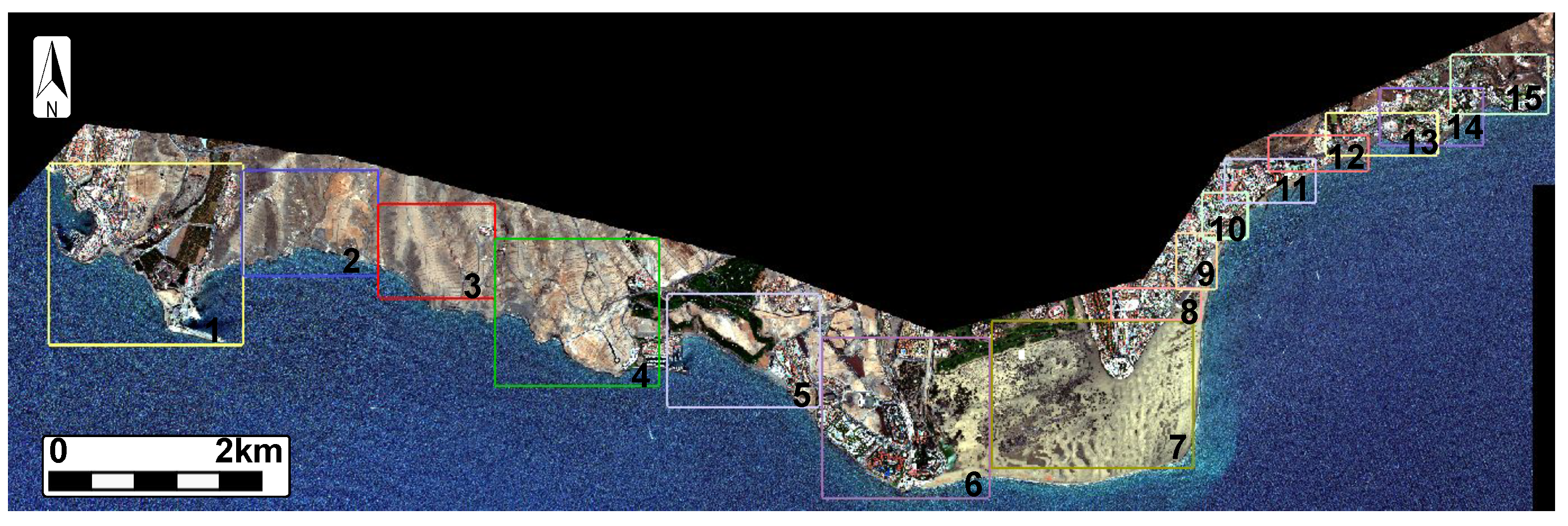
Figure 1. ROIs location projected over the WorldView-2 image of Maspalomas.
Remotesensing 14 05862 g001
Figure 2. Manual relabeling and correction of the dataset for semantic segmentation.
Remotesensing 14 05862 g002
Figure 3. Examples of the dataset after the manual relabeling process.
Remotesensing 14 05862 g003
Figure 4. RS-ESRGAN Generator architecture, with a sequence of Residual in Residual Dense Blocks (RRDBs) producing the dense feature extraction of the network. Source: [7].
Remotesensing 14 05862 g004
Figure 5. High-level scheme architecture of the SEG-ESRGAN.
Remotesensing 14 05862 g005
Figure 6. SEG-ESRGAN model to produce a super-resolution image and enhanced segmentation maps of remote sensing images.
Remotesensing 14 05862 g006
Figure 7. (a) Encoder sub-block of the SEG-ESRGAN segmentation branch and (b) Attention blocks that compose the scSE block.
Remotesensing 14 05862 g007
Figure 8. Central block of the SEG-ESRGAN.
Remotesensing 14 05862 g008
Figure 9. Decoder block of the SEG-ESRGAN.
Remotesensing 14 05862 g009
Figure 10. Results of a region of Maspalomas-2017 from the Test Set. (a) WorldView-2 GT, (b) Sentinel-2 bicubic interpolation, (c) SR with α = 0 , (d) SR with α = 0.1 , (e) SR with α = 0.3 , (f) SR with α = 0.5 , (g) SR with α = 0.7 , (h) SR with α = 0.8 , (i) SR with α = 1 . Image size: 200 × 200 pixels.
Remotesensing 14 05862 g010
Figure 11. Results obtained on the test set of the Maspalomas dataset: (a,f) Sentinel-2 bicubic input image; (b,g) WorldView GT; (c,h) SISR results; (d,i) SSSR GT, (e,j) SSSR results. The colormap is the same as depicted in Figure 2.
Remotesensing 14 05862 g011
Figure 12. Zoom results obtained on different locations from the Test Set of the dataset: (a) Sentinel-2 bicubic input image, (b) WorldView-2 GT, (c) SISR result, (d) SSSR GT, (e) SSSR result. The colormap is the same as depicted in Figure 2. Image size 200 × 200 pixels.
Remotesensing 14 05862 g012
Figure 13. Segmentation results from different models using the test subset. (a) GT image, (b) U-Net, (c) DeepLabV3+, (d) HRNet, (e) U-Net with SR inputs, (f) Dual_DeepLab, (g) Dual_DeepLab_RRDB, (h) SEG-ESRGAN. Image size: 200 × 200 pixels.
Remotesensing 14 05862 g013
Figure 14. SR comparative performance between: (a) Sentinel-2 bicubic image; (b) WorldView-2 GT; (c) Dual_DeepLab model; (d) Dual_DeepLab_RRDB model; (e) RS-ESRGAN inference, (f) SEG-ESRGAN model. Image size 200 × 200.
Remotesensing 14 05862 g014
Figure 15. SEG-ESRGAN inference of other WorldView-Sentinel pairs that do not belong to the dataset. (a) Sentinel-2 bicubic image, (b) WorldView GT, (c) SISR, (d) SSSR.
Remotesensing 14 05862 g015
Table 1. Sentinel-2 and WorldView-2 band spectral characteristics.
SatelliteSpectral BandCentral Wavelenght
(nm)
Bandwidth
(nm)
Sentinel-2B2: Blue49065
B3: Green56035
B4: Red66530
B8: Near-IR842115
WorldView-2B2: Blue48054.3
B3: Green54563.0
B5: Red66057.4
B7: Near-IR 183398.9
Table 2. RS-ESRGAN inference mean results on the test set of the Maspalomas dataset using different values of α . Best values in bold.
LR_BicSR_0SR_0.1SR_0.3SR_0.5SR_0.70SR_0.80SR_1.0
PSNR29.45231.00731.04730.76330.19629.57329.19528.203
SSIM0.7920.8240.8240.8190.8120.8020.7940.760
ERGAS 4.1883.5923.6023.6543.8094.0234.1674.632
SAM0.0670.0490.0500.0530.0560.0630.0660.079
Table 3. Confusion matrix, precision, F1-score and IoU results obtained with the test set of the Maspalomas dataset.
Classification Data123456Prec. F1IoUTotal Pixels
1Water0.99 00000.010.970.980.960136,030
2Vegetation00.76 00.180.030.030.810.790.647202,881
3Pool00.020.74 00.090.150.520.610.4393564
4Bare Soil0.010.0400.90 0.040.010.940.920.851712,037
5Asphalt0.010.1300.160.64 0.060.330.430.27432,974
6Built Soil00.10 0.030.040.100.730.690.710.55259,518
mean 0.710.740.62
weighted mean 0.890.880.7947
Table 4. Super-resolution metrics for the best model compared with the bicubic interpolation image. Best values in bold.
PSNRSSIMERGASSAM
Bicubic29.4520.7924.1880.067
SEG-ESRGAN30.7680.8163.6940.048
Table 5. Segmentation metrics obtained with the test set of the dataset. Best values in bold. mF1 refers to the mean F1 value, wF1 refers to the weighted mean F1 value and mIoU is the mean IoU.
F1mF1wF1mIoU
WaterVegetationPoolBare SoilAsphaltBuilt Soil
U-Net - WorldView (Upper Bound)0.970.820.700.930.570.740.78830.89440.6723
U-Net (bicubic)0.980.750.550.920.440.640.71330.86770.5904
DeepLabV3+ (bicubic)0.970.740.460.920.460.680.70500.86710.5826
Dual_DeepLab (bicubic)0.980.780.440.920.380.630.70640.86370.5870
HRNet (bicubic)0.980.750.530.890.420.670.70670.85000.581
Dual_DeepLab_RRDB (bicubic)0.980.780.530.920.410.680.71330.87170.5951
U-Net+SR*0.980.760.570.910.450.670.72330.86510.6003
SEG-ESRGAN (bicubic)0.980.790.610.920.430.710.74000.87830.6278
* U-NET+SR is trained and inferred with SR images of the dataset (α = 10%).
Table 6. Super-resolution metrics obtained with the test set of the dataset. Best values in bold.
PSNRSSIMERGASSAM
Bicubic29.4520.7924.1880.067
U-Net+SR *31.0470.8243.6020.050
Dual_DeepLab30.3720.8073.7790.050
Dual_DeepLab_RRDB30.5630.8113.7500.048
SEG-ESRGAN30.7680.8163.6940.048
* U-NET+SR is trained and inferred with SR dataset (α = 10%).
Table 7. Number of parameters and memory consumption of each model.
SegmentationSuper-ResolutionTrainable Parameters (M)Estimated Memory (MB)
Dual_DeepLabXX51.4102.861
Dual_DeepLab_RRDBXX47.394.597
U-Net with ResNet-101X 51.5103.034
ESRGAN X16.633.251
SEG-ESRGANXX30.861.522
Table 8. WorldView and Sentinel-2 pairs for Maspalomas (Gran Canaria, Spain).
YearSentinel-2WorldView-2WorldView-3WV Resolution
201529 September4 June-2.0 m
201731 May-31 May1.6 m
Publisher’s Note: MDPI stays neutral with regard to jurisdictional claims in published maps and institutional affiliations.