Article

Developing an Automated Python Surface Energy Balance System (PySEBS) Software for Calculating Actual Evapotranspiration-Software Development and Application Case in Jilin Province, China

1
College of Land Science and Technology, China Agricultural University, Beijing 100193, China
2
Key Laboratory of Arable Land Conservation in North China, Ministry of Agriculture and Rural Affairs, Beijing 100193, China
3
USDA-ARS Conservation and Production Research Laboratory, Bushland, TX 79012, USA
*
Author to whom correspondence should be addressed.
Remote Sens. 2022, 14(21), 5629; https://doi.org/10.3390/rs14215629
Submission received: 12 September 2022 / Revised: 26 October 2022 / Accepted: 4 November 2022 / Published: 7 November 2022

Abstract

:
In this study, Python Surface Energy Balance System (PySEBS) software was developed in the Python 2.7 programming language for continuous calculation of actual evapotranspiration (ETa) at regional scales. The software is based on the Surface Energy Balance System (SEBS) model, which uses basic meteorological data, MODIS remote sensing data, and Digital Elevation Model (DEM) data as the original input data and finally outputs daily-scale ETa in the form of raster data with a spatial resolution of 1 km × 1 km. To verify the reliability of the PySEBS model, the ETa of spring maize during the growing season in Jilin Province, China, from 2001 to 2020 was calculated and analyzed in this study and compared with the results of similar studies by others. The findings showed that the PySEBS model has a reasonable accuracy in estimating ETa within ±15% and is a robust model that can achieve the continuous calculation of ETa at a regional scale. Therefore, PySEBS software is a useful tool for regional irrigation scheduling and water resources management.

1. Introduction

Actual evapotranspiration (ETa) is the combined term for ground evaporation and vegetation transpiration. ETa is an important component of water balance for agricultural fields and is widely used in many areas, such as agronomy, hydrology, ecology, meteorology, and environmental science [1,2,3,4]. The influencing factors include meteorological factors such as solar radiation, air temperature, relative humidity, and wind speed. In addition, it is also related to vegetation type, growth condition, and soil properties [5]. The concept closely related to ETa is the reference crop evapotranspiration (ETo) [6,7]. The FAO Penman–Monteith approach was developed by defining the ETo as evapotranspiration from a broad surface of highly uniform, vigorously growing, well-watered green grass, assuming a surface resistance of 70 s m−1, a height of 0.12 m, and an albedo of 0.23 [7].
Since the establishment of Dalton’s theorem in 1802, different methods for estimating ETa have emerged. Bowen et al. [8] proposed the Bowen ratio-energy balance method for ETa calculation in 1926, according to the energy balance equation. Thornthwaite and Holzman [9] proposed an aerodynamic method for calculating ETa based on the boundary layer similarity theory. In 1948, Penman proposed the concept of “evaporation force” and established the joint ETa equation [10]. Monteith [11] derived the famous Penman–Monteith equation in 1965, which opened up a new way to study evaporation from an unsaturated subsurface. Allen et al. [7] used the method of assigning a reference crop canopy resistance and a fixed height to give a careful description of the use of the P-M formula under different environmental conditions. Subsequently, many studies of stratified models of ETa were carried out based on the energy balance principle. The single-layer model mainly uses the energy balance residual method, which does not distinguish between soil evaporation and vegetation transpiration in the estimation process. It uses a holistic approach to estimate ETa, but this method usually results in overestimation under sparse vegetation. Therefore, Shuttleworth and Wallace [12] proposed a two-layer model based on the theoretical principle of the P-M formula, in which soil evaporation and vegetation transpiration are calculated separately. Based on Shuttleworth’s two-layer model, Dolman [13] proposed a three-layer model, and Choudhury et al. [14] put forward a four-layer model. Norman et al. [15] developed a two-source model for row crops. All the above methods for calculating ETa are mainly based on point-source data, which is relatively accurate on small scales. However, in practice, it is often necessary to know the ETa on a large scale, and the traditional methods can hardly meet the requirements. The gradual rise of remote sensing technology in the late 1960s, especially the application and development of thermal infrared remote sensing, can achieve the conversion from point to surface, which makes the large-scale study of ETa possible.
A series of remote sensing models for accurate estimation of ETa have emerged, such as the triangle method model, Surface Energy Balance Algorithm for Land (SEBAL), Surface Energy Balance Systems (SEBS), Mapping Evapotranspiration with Internalized Calibration (METRIC), Two source Trapezoid Model for Evapotranspiration (TTME), Google Earth Engine SEBAL (geeSEBAL), etc. [16,17,18,19,20,21]. Du et al. [22] used the SEBAL model, combined with remote sensing data and meteorological data, to estimate the water productivity and specific water consumption of rice in the Songnen Plain. Bhattarai and Liu [23] developed a Matlab-based toolbox named LandMOD ET mapper to run SEBAL and METRIC on Landsat and MODIS images for mapping field to regional scale ETa. The SEBALIGEE model developed by Mhawej and Faour [24] is an automated, user-friendly, flexible, and open-access 30 m ET retrieval system. Its main features are the estimations of ET and Kc in diverse climatic regions with readily available Landsat-8 30-m satellite images. Ramirez-Cuesta et al. [25] developed a new ArcGIS toolbox for implementing the METRIC energy balance model, called Metric-GIS, and tested it in a semi-arid environment. Ellsasser et al. [26] developed the QWaterModel tool based on the DATTUTDUT energy balance model using land surface temperature maps as input, making ET predictions available to a wider audience. Wu et al. [27] introduced an ETWatch Cloud service, which is a model collection migrated from a local PC to the cloud platform for ET generation using readily available RS and standard ground-based meteorological observations. Laipelt et al. [21,28] developed the geeSEBAL software in the Google Earth Engine environment based on the SEBAL algorithm and achieved better results in the calculation of evapotranspiration in the Brazilian region. Huang et al. [29] and Ren et al. [30] used the SEBS model, combined with MODIS data, to estimate the water productivity and water consumption of maize. The results showed that the improved SEBS model could be well applied to the study of ETa in dryland farming.
Although there are some tools for calculating ETa at a regional scale, such as ILWIS (Integrated Land and Water Information System) software, the operation process is complicated for users [31]. The purpose of this study is to introduce the Python Surface Energy Balance System (PySEBS) software for calculating ETa at a regional scale to simplify the complex process of ETa calculation and to achieve multi-year, continuous, automatic, and efficient estimation of ETa. Moreover, a case study is performed, and the results of calculated ETa using this software are described, analyzed, and compared to similar studies.

2. Materials and Methods

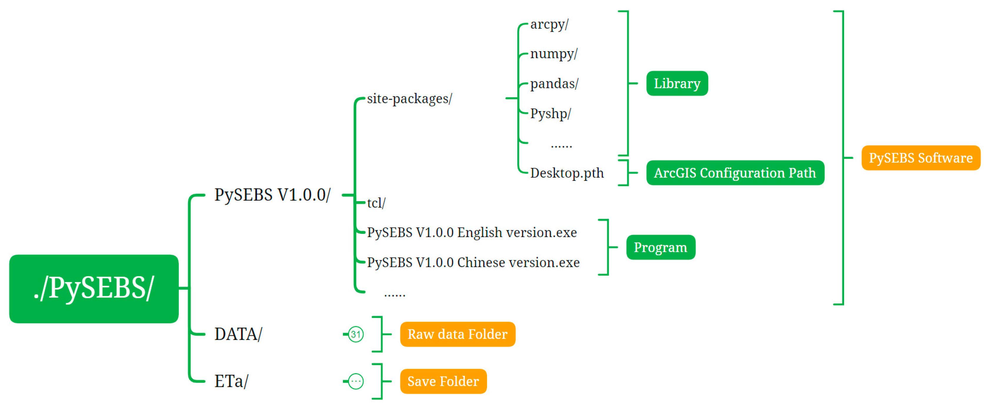
2.1. Installing the PySEBS and Software Requirements

The PySEBS is software that can be used to calculate actual evapotranspiration (ETa) on a spatial scale based on the Surface Energy Balance System model (SEBS). The software is written in Python 2.7.14 due to Python (2.7) being the latest version supported by ArcGIS 10.1–10.6. Since ETa is calculated on a spatial scale, the software operation utilizes some of the built-in tools in ArcGIS, and the proper operation of these tools depends on the calling of the Arcpy package in ArcGIS. Therefore, the user needs to ensure that the ArcGIS software is installed successfully.
The PySEBS software is compressed into a PySEBS V1.0.0.zip file. The schematic diagram of the PySEBS file structure is shown in Figure 1. The schematic box labeled. /PySEBS/represents a folder named PySEBS in the working directory, where the PySEBS 1.0.0.zip file will be stored after extraction. The PySEBS folder contains two parts: the PySEBS V1.0.0.exe program; and the site-packages folder containing the code libraries (arcpy package, numpy package, pandas package, Pyshp package, etc.) and the configuration Desktop.pth file.

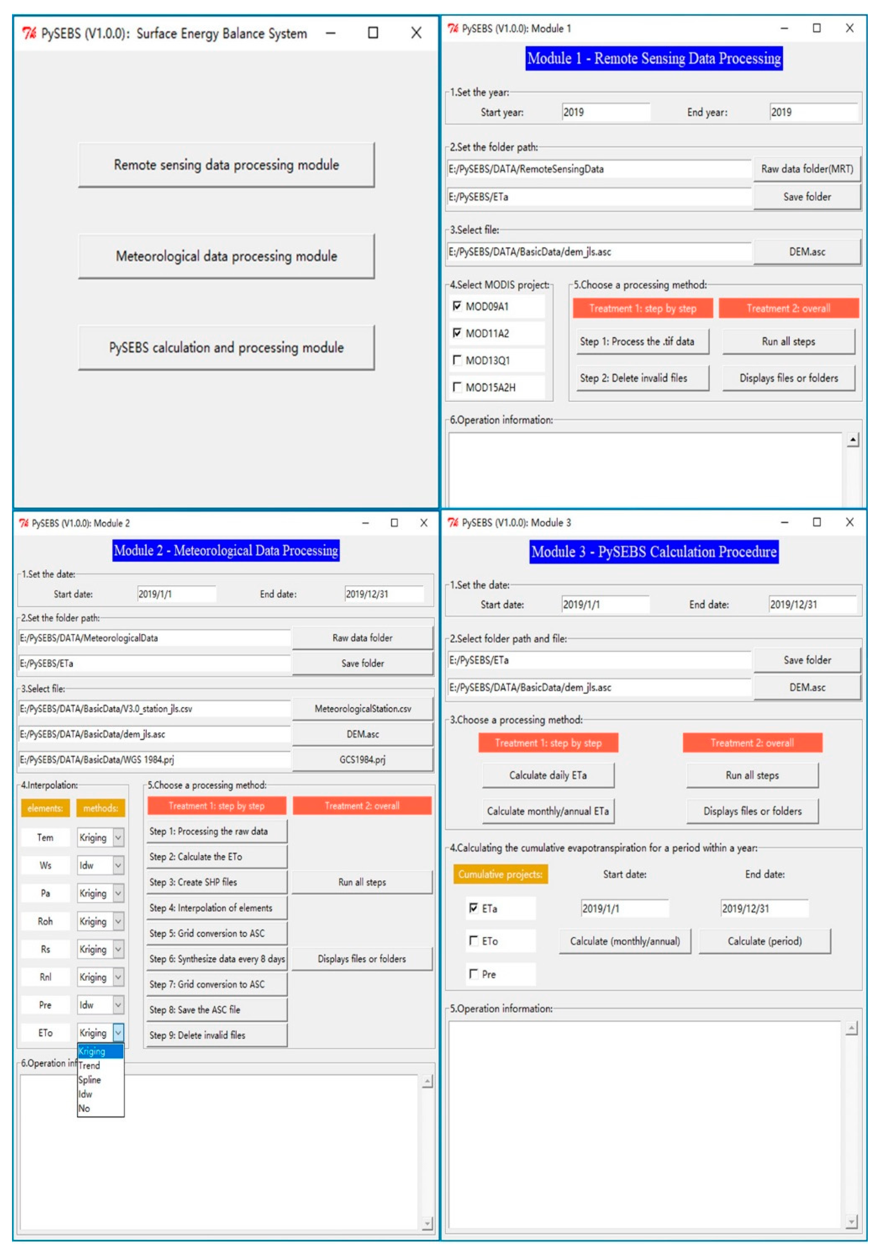
2.2. Graphical User Interface Introduction

The PySEBS software is a concise and straightforward scientific computing tool. It contains one main interface and three sub-interfaces (Figure 2). The main interface consists of three button controls: the remote sensing data processing module button, the meteorological data processing module button, and the PySEBS calculation and processing module button. Each button control accesses the corresponding module (sub-interface): Module 1-Remote Sensing Data Processing interface, Module 2-Meteorological Data Processing interface, and Module 3-PySEBS Calculation Procedure interface.
The main functions of Module 1 and Module 2 are to provide properly processed and formatted input data for use in Module 3. Module 3 is used to calculate ETa on a daily/monthly/annual scale, or for any period of time within a year and across years, based on the input data (raster data) prepared by Modules 1 and 2. There is no processing priority between Modules 1 and 2. Moreover, there are common properties configured for all three modules, including the time setting of the start and end year, file and folder pathway settings, selection of processing method, and information output.
Each module is described below, and detailed descriptions are available in the PySEBS V1.0.0 Actual Evapotranspiration (ETa) Calculator User’s Guide in the Supplementary Materials:
Module 1 is used to process remotely sensed data and generate the daily data files in .asc format for input into Module 3. Module 1 can only process data on an annual basis, and therefore the user must arrange the downloaded remote sensing files in specific folders by data type and by year. The downloaded remote-sensed data needs to be pre-processed before it can be used in the PySEBS program. For demonstration, remotely sensed data were obtained from the National Aeronautics and Space Administration (NASA, http://modis-land.gsfc.nasa.gov/ (accessed on 9 March 2019)). In this example, images h26v04 and h27v04 were downloaded, and the MRT (MODIS Reprojection Tool) projection tool was applied to preprocess the data for merging, resampling, format conversion, etc., and Cygwin software was used for batch processing (see Table 1 for specific parameters). The purpose of pre-processing is to convert the remote sensing data from the hierarchical data format (.hdf) to raster files (.tif). The location of the .tif file will be in the same folder as the .hdf file, and the name of the preprocessed .tif file must contain the date information string (seven digits) of the corresponding data; an example file name is MOD09A1_2019001.sur_refl_b01.tif.
The function of Module 2 is to process the meteorological data and generate the daily file in the .asc format that is required by Module 3. The meteorological data used in this study is China’s surface climate data daily value data set (V3.0), which is derived from the National Meteorological Information Center (http://data.cma.cn/site/index.html (accessed on 30 May 2018)); the platform contains the daily meteorological data from 824 reference weather stations. The meteorological data in the dataset includes atmospheric pressure, air temperature, precipitation, evaporation, sunshine hours, surface temperature, wind speed and direction, and relative humidity at each station. The downloaded original meteorological data is in .txt format and includes all meteorological stations in each folder that need to be preprocessed. Once the downloaded V3.0 weather datasets are placed in the same folder, Module 2 can be used to process the raw data directly. If meteorological datasets from other sources are used, they need to be organized in .csv format and stored in the 1RawData folder. An example of the corresponding path may be: .\PySEBS\ETa\2MeteorologicalData\1RawData\2019.csv.
Module 3 uses the daily input data (in .asc format) generated by Module 1 and Module 2 to calculate ETa on a daily/monthly/annual basis, or for a specified period of time. The PySEBS model requires 15 necessary parameters. Module 1 provides eight essential parameters, including seven parameters from MOD09A1 (Band1, Band2, Band3, Band4, Band5, Band7, and Szen), and one parameter from MOD11A2 (Lst). Module 2 provides seven essential parameters, including the Digital Elevation Model (DEM) parameter and six meteorologically related parameters (Tem, Ws, Pa, Roh, Rs, and Rnl). Moreover, there are two non-essential parameters, Pre and ETo, which are not involved in the PySEBS calculation process.

2.3. PySEBS Software Theoretical Foundation

The SEBS model, as proposed by Su, is a single-layer model based on the surface energy balance principle [18], which consists of four components: (1) The determination of the land surface physical parameters based on the remotely sensed spectral reflectance and radiance; (2) The estimation of the roughness length for heat transfer; (3) The calculation of sensible heat flux; and (4) The calculation of latent heat flux. Compared with other single-layer models based on the energy balance principle, the PySEBS model has the advantage that the data in each grid is calculated independently, so that even if some grids have missing data on a certain day due to the influence of rain and clouds, the calculation in other grids will not be affected; this can maximize the utilization of the remote sensing data.
The net earth’s surface radiation is the basis of various energy exchanges and can be divided into three parts: (1) the soil heat flux that warms the soil; (2) the sensible heat flux that warms the atmosphere; and (3) the latent heat flux of evapotranspiration (the latent heat of soil evaporation and crop transpiration). The main equations for surface energy balance are as follows, and the detailed derivation of the equations can be found in the relevant literature reviewed [7,18,31,32,33,34,35,36,37,38,39,40,41,42] and in the Supplementary Materials:
R n = G 0 + H + λ E ,
where Rn is the net radiation (W m−2), G0 is the soil heat flux (W m−2), H is the sensible heat flux (W m−2), and λE is the latent heat flux (W m−2), in which λ is the latent heat of evaporation (J kg−3) and E is the actual evapotranspiration (mm d−1). After calculating each parameter of the surface energy balance separately, the actual daily ETa can be obtained according to the constant evaporation ratio within one day.
Calculations of net radiation Rn:
R n = ( 1 α ) R s w d + ε R l w d ε σ T 0 4 ,
where α is surface albedo, a ratio of radiation reflected by the surface to global radiation (a sum of direct solar radiation and scattered radiation); Rswd and Rlwd (W m−2) represent downward solar radiation and downward long-wave radiation, respectively; ε is surface emissivity and can be classified into εland (surface emissivity of land) and εwater (surface emissivity of water) according to different underlying surfaces; σ is the Stephan Boltzmann constant equal to 5.67 × 10⁻⁸ (W m−2 K−2); and T0 is the surface temperature (K).
Calculations of soil heat flux G0:
G 0 = R n [ Γ c + ( 1 f c ) ( Γ s Γ c ) ] ,
where Γc is the ratio of soil heat flux to net radiation in the condition of total vegetation cover, (Γc = 0.05), and Γs is a ratio of soil heat flux to net radiation in the condition of bare soil (Γs = 0.315); ƒc is vegetation coverage inversed through remote sensing data.
Calculations of sensible heat flux H:
H = ρ C p θ 0 θ a r a ,
r a = 1 k u [ ln ( z d 0 z 0 h ) Ψ h ( z d 0 L ) + Ψ h ( z 0 h L ) ] ,
where ρ for air density (kg m−3); Cp for constant-pressure specific heat (J kg−1 K−1); θ0 for latent surface temperature (K); θa for latent air temperature (K) at an elevation of z; ra for external resistance; k for Karman constant (k = 0.4); u for friction velocity (m s−1); z for reference measured elevation (m), generally between 2 and 10 m; d0 for zero plane displacement height (m); z0h for scalar roughness height for heat transfer (m); Ψh for stability correction coefficients of heat exchange MOS; and L for Obukhov length (m).
Calculations of daily evapotranspiration Edaily:
The previously calculated net surface radiation, soil heat flux, and sensible heat flux are based on the instantaneous values at the moment of satellite transit. In contrast, in the PySEBS model, the daily evapotranspiration is calculated from the evaporation ratio with the daily average net radiation and daily average soil heat flux. The evapotranspiration ratio remains stable throughout the day [43,44,45,46], and assuming that the evapotranspiration ratio is constant throughout the day, the daily evapotranspiration is calculated by the following equation:
E d a i l y = 8.64 10 7 Λ 0 24 R n ¯ G 0 ¯ λ ρ w ,
R n ¯ = ( 1 α ) K 24 + ε L 24 ,
G 0 ¯ 0 ,
In the above equation, Edaily stands for the actual daily evapotranspiration (mm day−1); 8.64∙107 stands for a unit conversion coefficient; Λ 0 24 stands for the daily mean evaporation ratio that can be substituted by the evaporation ratio Λ figured out by the PySEBS model; R n ¯ stands for the daily mean net radiation flux (W m−2); and G 0 ¯ stands for the daily mean soil heat flux (W m−2), considering that the amount of heat absorbed and released by soil is approximately equal during the day, the daily mean soil heat flux is set to 0. Additionally, λ refers to the latent heat of vaporization of water and λ = 2.45∙106 (J kg−1); ρw refers to the density of water and ρw = 1000 (kg m−3); α is the surface albedo; K 24 refers to incident global radiation (W m−2), which is obtained through the unit conversion of the incident solar radiation (MJ m−2 day−1) expressed in the Penman–Monteith equation; ε is surface emissivity; and L24 refers to daily net outgoing long-wave radiation (W m−2), which is obtained through the unit conversion of the net long-wave radiation (MJ m−2 day−1) expressed in the Penman–Monteith equation.

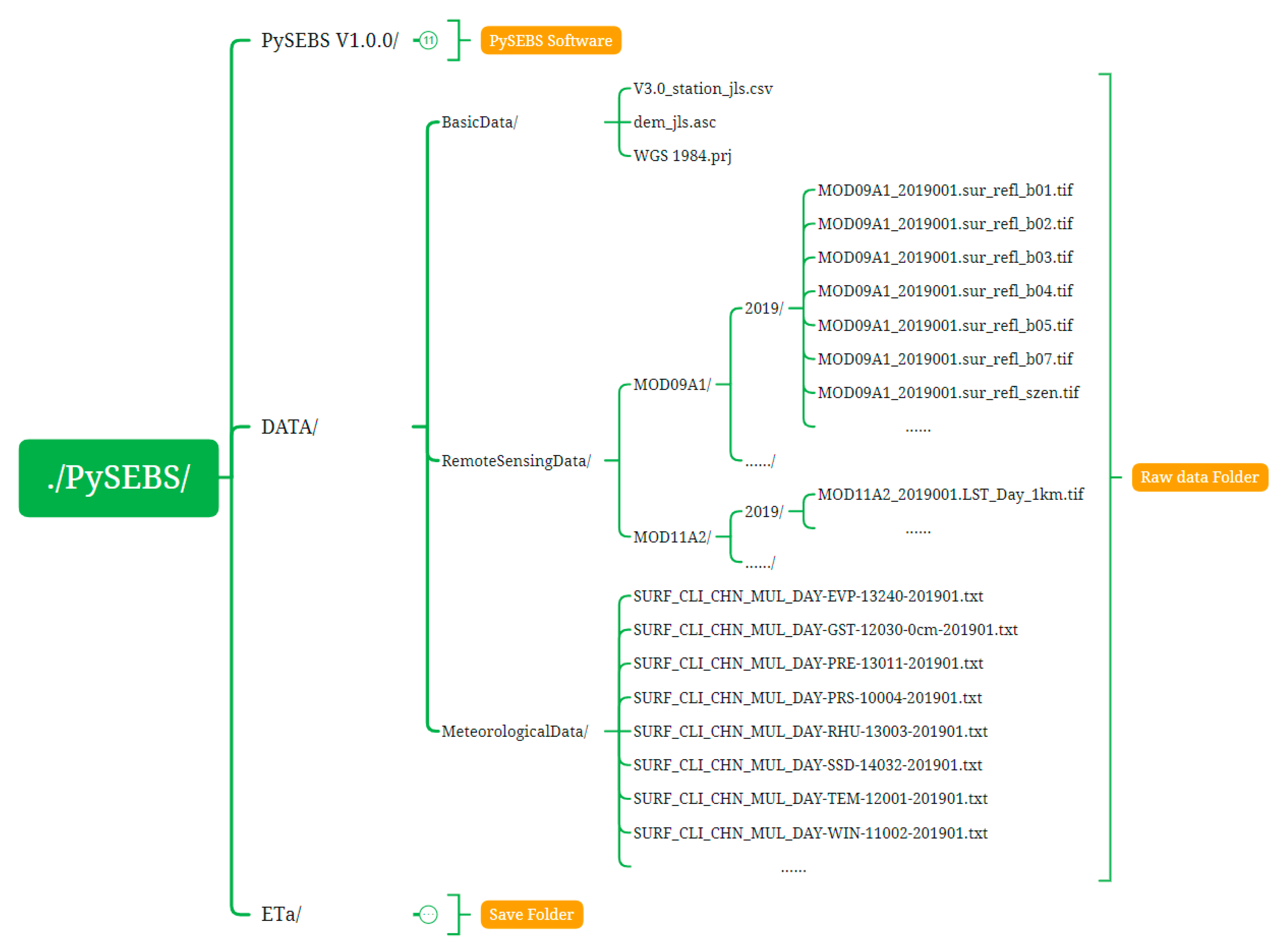
2.4. Initial Input Data
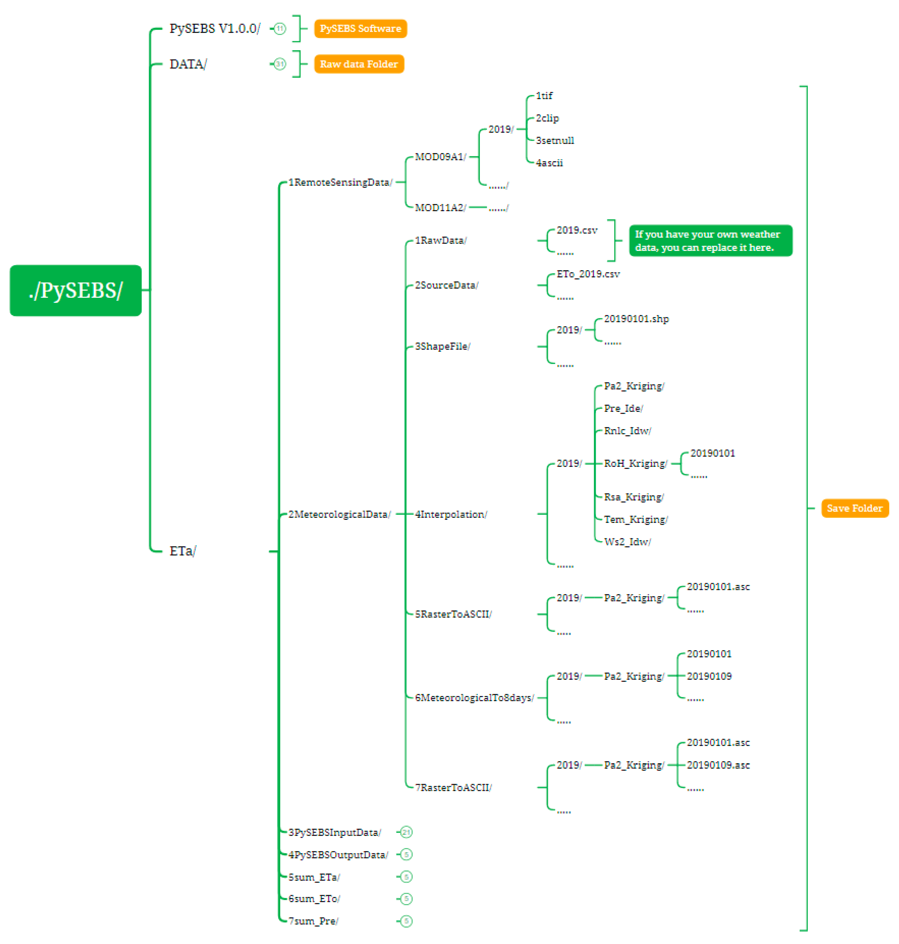
Input data required by Modules 1, 2, and 3 can be divided into three parts: the first part is the basic data, which includes the information file (V3.0_station_jls.csv) of weather stations for the V3.0 meteorological dataset within the study area, the study area DEM file (dem_jls.asc), and the geographic coordinate system file (WGS 1984.prj); the second part is the remote sensing data, which includes MOD09A1 and MOD11A2; the third part is the meteorological data, which includes the raw data of the V3.0 meteorological dataset. Meteorological data from other sources can also be used; the data needs to be prepared by the users following the format of 2019.csv and located in the corresponding folder.
The input data or files described above are all saved in the designated folders. Each module is connected to the file or folder so that the data can serve as the input for the module. Specifically, the basic data is connected in the form of files; remotely sensed data and meteorological data are connected in the form of subdirectory.
The structure diagram of the path to the initial input data is shown in Figure 3. The path to the basic data is ./PySEBS/DATA/BasicData/. The path to the remote sensing data is ./PySEBS/DATA/RemoteSensingData/MOD09A1/2019/ and ./PySEBS/DATA/RemoteSensingData/MOD11A2/2019/. The meteorological data is saved in the path: ./PySEBS/DATA/MeteorologicalData/.

2.5. Output Results

The ./PySEBS/ETa/ file path is a user-defined folder to save the output results, which will be created automatically if such a folder does not exist in the project directory. The folder 1RemoteSensingData/ is used to save the intermediate files generated during the remote sensing data processing in Module 1. The folder 2MeteorologicalData/ is used to save the intermediate files generated during the meteorological data processing in Module 2. The folder 3PySEBSInputData/ is used to save the final processing results of remote sensing and meteorological data. In addition, the folder 3PySEBSInputData/ also serves as the path for input files for Module 3. The 4PySEBSOutputData/ folder will store the daily ETa results, and the 5sum_ETa/ folder will store the monthly and annual ETa results calculated by Module 3 (Figure 4). The 6sum_ETo/ folder and the 7sum_Pre/ folder are used to store cumulative reference evapotranspiration and precipitation, respectively.
As mentioned earlier, if meteorological data derived from other sources need to be used, the data must be prepared in the required format (Figure 5) and stored in the file path 2Meteorologicaldata/1RawData/ to replace the V3.0 meteorological data. The files in the file path 2MeteorologicalData/2SourceData/ (e.g., ETo_2019.csv) used the data in the 2Meteorologicaldata/1RawData/ folder as input and calculated the ETo and its process variables; the purpose of these files is to provide the six required meteorological parameters for Module 3. The calculation of ETo is also a strength of this software, if the users need to use ETo and other parameters in the calculation process, the information can be found in the folder 2MeteorologicalData/2SourceData/.
The 3PySEBSInputData/ folder stores the final processing results calculated from Module 1 and Module 2 and the input files from Module 3. The files are stored in the form of one folder per day and contain 15 .asc files that are required for the PySEBS model calculation and one optional precipitation file (pre.asc). The required parameters include one DEM file (dem.asc), seven MOD09A1 files (band1.asc, band2.asc, band3.asc, band4.asc, band5.asc, band7.asc, and szen.asc), one MOD11A2 file (lst.asc), and six meteorological parameter files (tem.asc, ws.asc, pa.asc, roh.asc, rs.asc, and rnl.asc) (Figure 6).

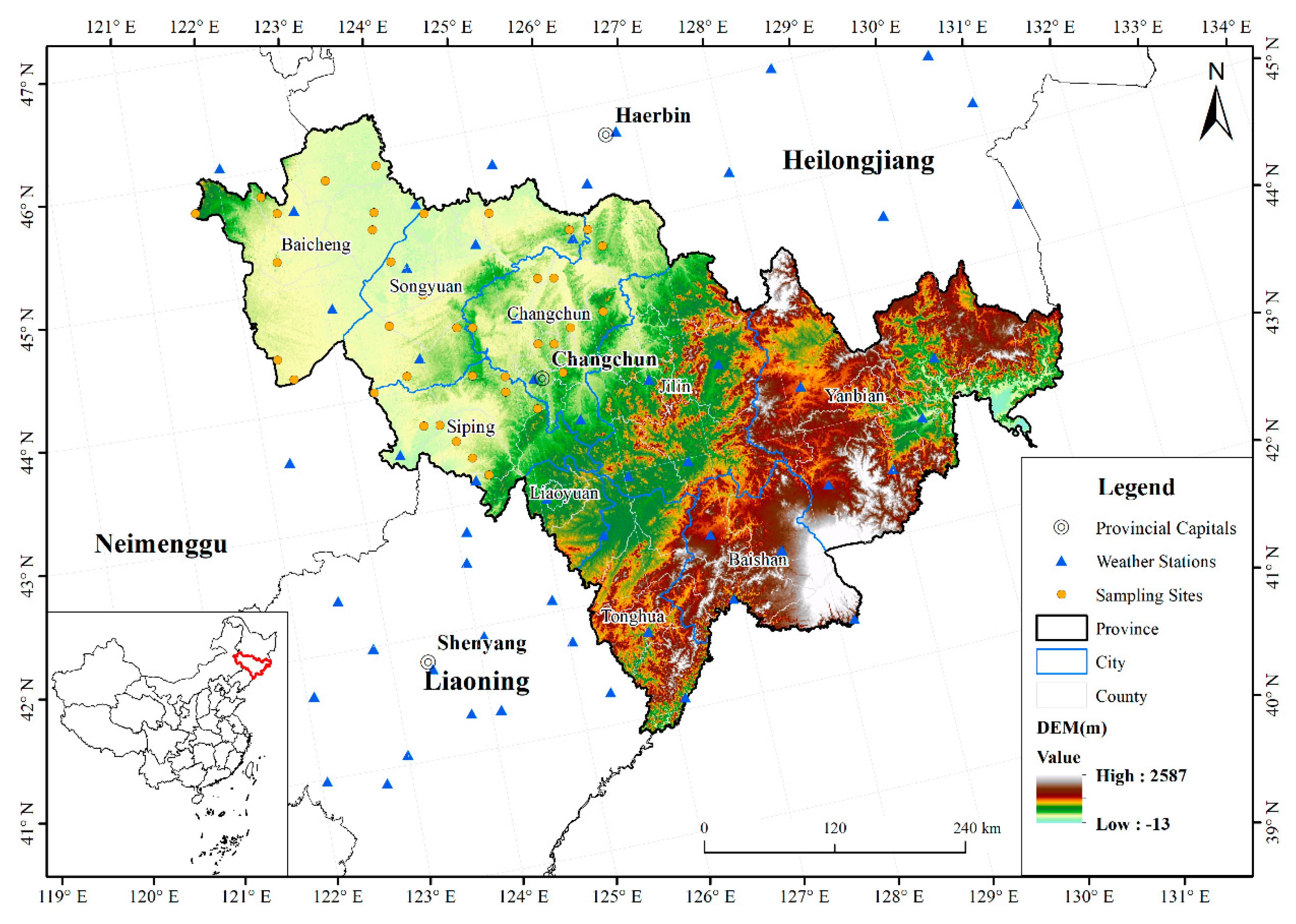
2.6. PySEBS Case Study-Study Area

After the development of PySEBS software, the ETa was calculated for spring maize in Jilin Province from 2001 to 2020, and the ETa was analyzed at both temporal and spatial scales during the growing season of spring maize in this study. Jilin Province is located in the central part of northeastern China (Figure 7). The terrain map shows obvious characteristics of high elevations in the southeast and low elevations in the northwest. The latitude varies from 40°50′ to 46°19′N, and the longitude ranges from 121°38′ to 131°19′E. Jilin Province is 769.6 km long from east to west and 606.6 km wide from north to south and has an area of 187,400 km2. As for climate conditions, it belongs to a temperate continental monsoon climate with four distinct seasons. Rain and heat are in the same season, such as a rainy summer with high temperatures and a cold and dry winter. The average winter temperature is below −11 °C, and the average summer temperature is above 23 °C. The annual average sunshine hours are 2259–3016 h. The annual average precipitation is 400–600 mm, and the annual frost-free period is 120–160 days. The climatic conditions of Jilin Province make it an important commodity grain production region in China. Due to the geographical advantage for agriculture, it has become one of the three famous Corn Belts in the world.

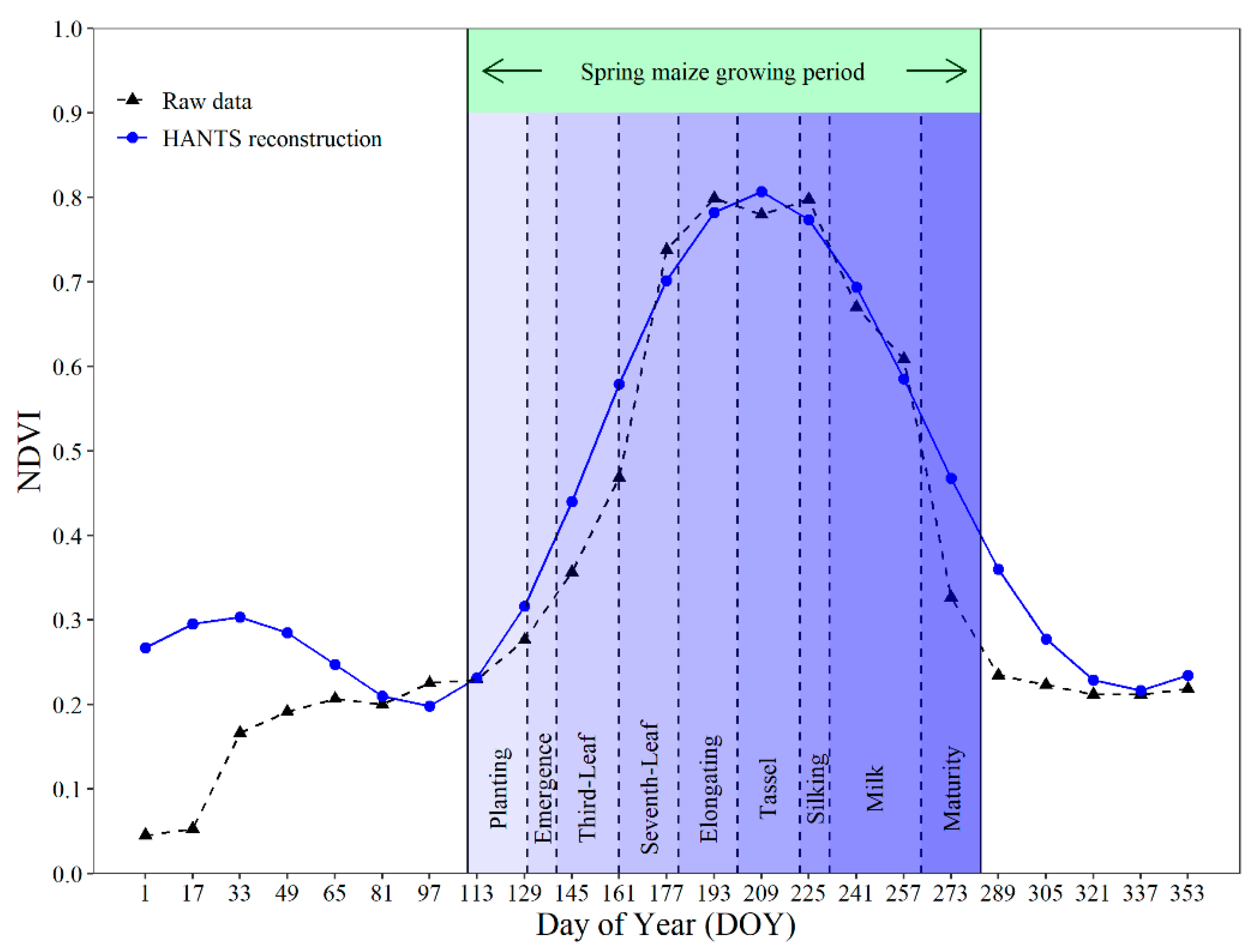
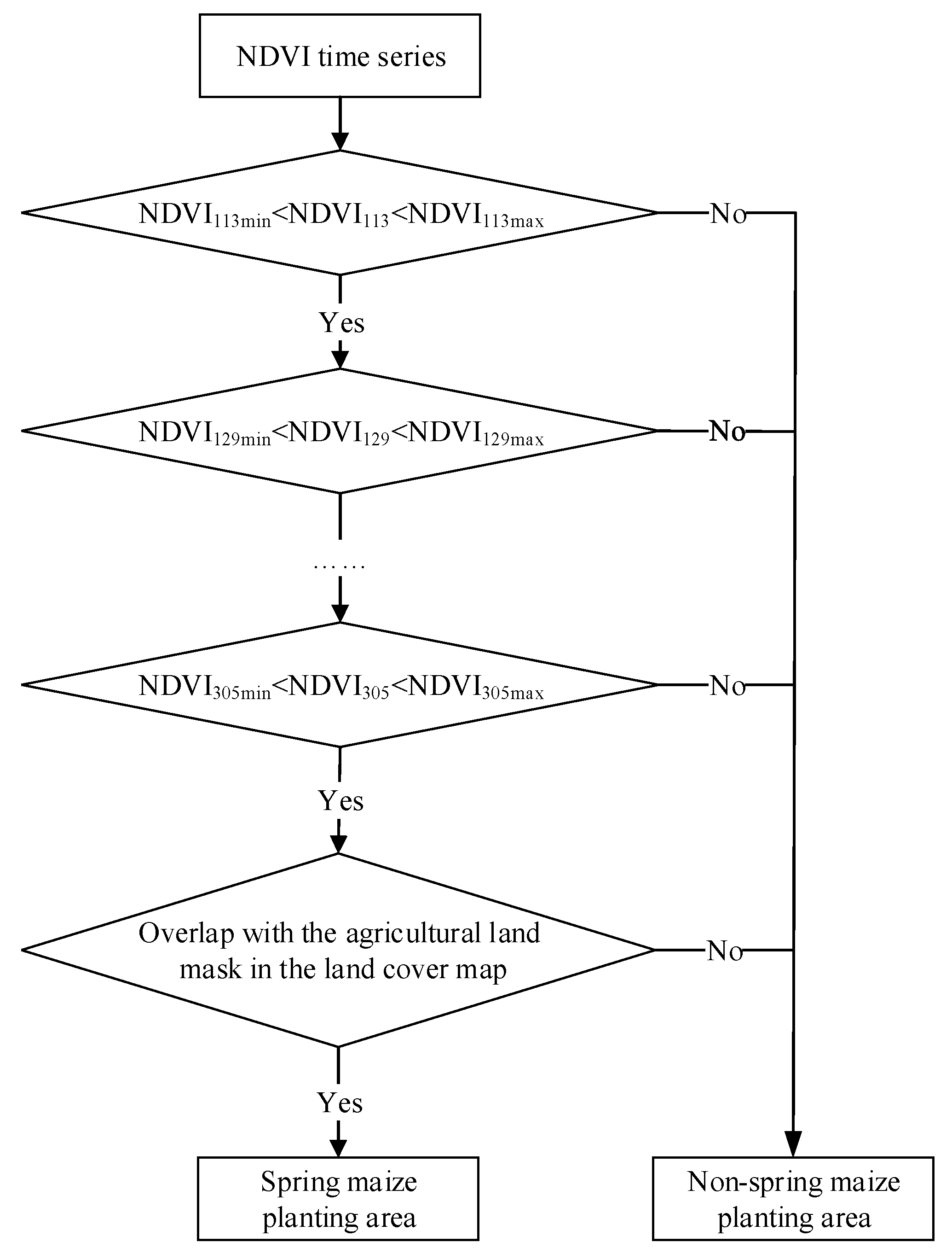
2.7. Calculation of ETa during Spring Maize Growing Season

The ETa of spring maize was calculated by PySEBS software. The data used were remote sensing data, meteorological data, and DEM data. The remote sensing data were obtained from NASA. The meteorological data are the daily data set of China’s surface climate data (V3.0), which were accessed from the Chinese National Meteorological Information Center. The digital elevation data ASTER GDEM V2 were downloaded from the geospatial data cloud (http://www.gscloud.cn/ (accessed on 16 May 2018)) with a spatial resolution of 30 m × 30 m.
In the process of calculating ETa through the PySEBS model in this study, the weather data were synthesized for 8 days due to the remote sensing data of MOD09A1 and MOD11A2 used are 8-day synthesis products. Then, the weather data and remote sensing data with a unified time scale were used as the input parameters of the PySEBS model. Finally, the 8-day synthetic ETa was obtained. Then, according to the start and end time of the growth period of spring maize (1 May to 30 September), the ETa during the growth period was accumulated by adding up.

3. Results

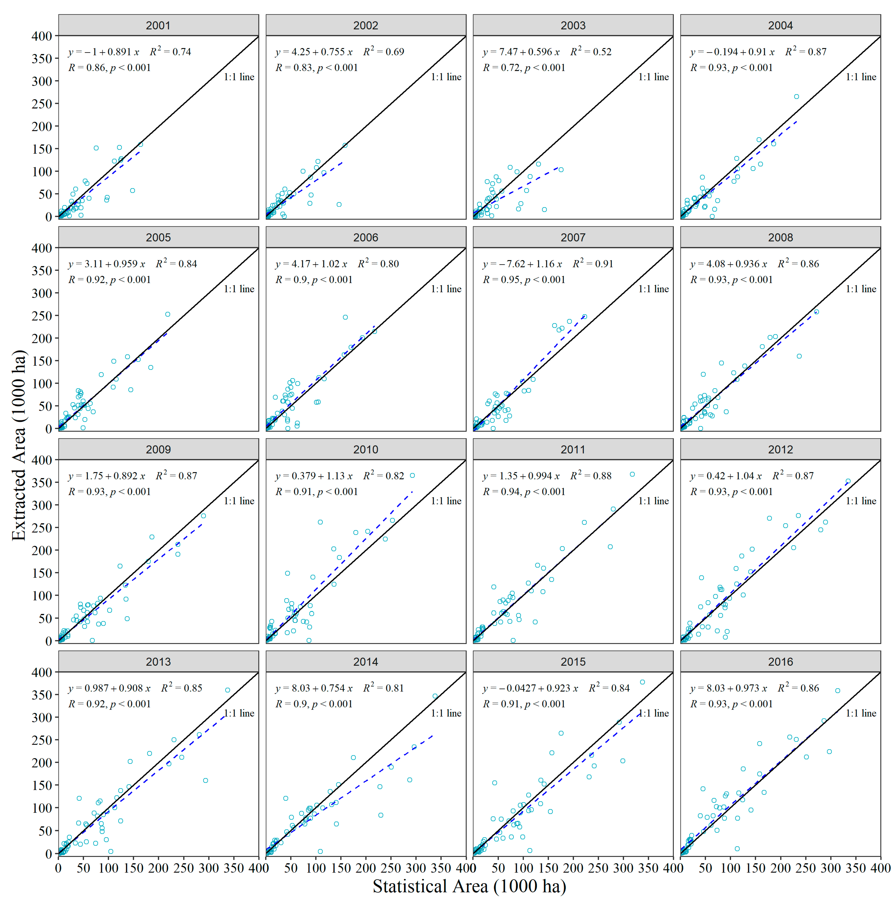
3.1. Extraction of Planting Area

The PySEBS software is a software for the calculation of the ETa on a spatial scale, and the results of the calculation are finally presented in the form of a raster dataset. Since the subject of research in this study is spring maize in Jilin Province, the planting area of spring maize in the study area needs to be determined first.
According to the distinct spectral characteristics of spring maize in different growth stages, the Normalized Difference Vegetation Index (NDVI) can effectively reflect the differences between various crops. Based on the curve of the MODIS-NDVI time series and the land use data of Jilin Province over 16 years, a decision tree classification model was constructed to achieve the extraction of the spring maize planting area. To obtain time series curves of NDVI of spring maize in Jilin Province for all years, the NDVI values of each sampling site were extracted as the main basis for extracting the spring maize planting area using the coordinate information of 38 sample sites with a long-term spring maize planting in this study (Figure 7).
After the sowing and emergence stages, the NDVI showed an increasing trend, which rose rapidly during the three-leaf, seven-leaf, and jointing stages of the spring maize vegetative growing period. When the spring maize entered the tasseling stage at the peak of vegetative growth, the NDVI value reached its peak. Then, spring maize entered the reproductive growth stages of the silking period, milk maturity period, and maturity period, during which the NDVI values gradually decreased. To eliminate the influence of noise on the NDVI values, the method of Harmonic Analysis of Time Series (HANTS) was used to smooth the time series of MODIS-NDVI. The comparison of before and after processing curves is shown in Figure 8.
The construction of the decision tree for the extraction of the spring maize planting area in Jilin Province was based on the minimum and maximum time series curves of NDVI for the period of 2001 to 2016. A total of 13 images of NDVI values reconstructed by HANTS using a day-of-year (DOY) calendar from DOY 113 to 305 over 16 years were selected for this study. The pixels between the minimum and maximum NDVI values of the corresponding DOY were the candidate areas for the spring maize planting area. To eliminate the influence of other land uses, the agricultural land in the land cover map provided by the remote sensing data of MCD12Q1 was extracted as a mask. Finally, the spring maize planting area was obtained. The extraction process is shown in Figure 9.
In this study, the identification of the spring maize planting area was based on the NDVI time series curve for the period of 2001 to 2016. Except for 2003 and 2014, the extraction area and statistical area of 56 counties and districts in Jilin Province were basically evenly distributed on both sides of the 1:1 line, indicating that the constructed decision tree could better extract the planting area of spring maize (Figure 10). The relative error of spring maize area extraction from 2001 to 2016 was −4.15%. The lowest extraction accuracy over the years was above 80%, and the average extraction accuracy reached 90.60%. The coefficient of determination (R2) values of the statistical area and the extracted area of spring maize were greater than 0.8 except for 2001 to 2003, and the overall R2 was 0.81, which indicated that the extraction method of the spring maize area used in this study fit well with the actual situation.
The map of the multi-year average spring maize planting area in Jilin Province was obtained by accumulating the raster files of planting areas in previous years, and a raster was considered to belong to the multi-year average spring maize planting area when the number of years in which a raster appeared exceeded 7 years. This planting area map was used to clip the ETa raster data of Jilin Province calculated by PySEBS software to obtain the ETa of spring maize.

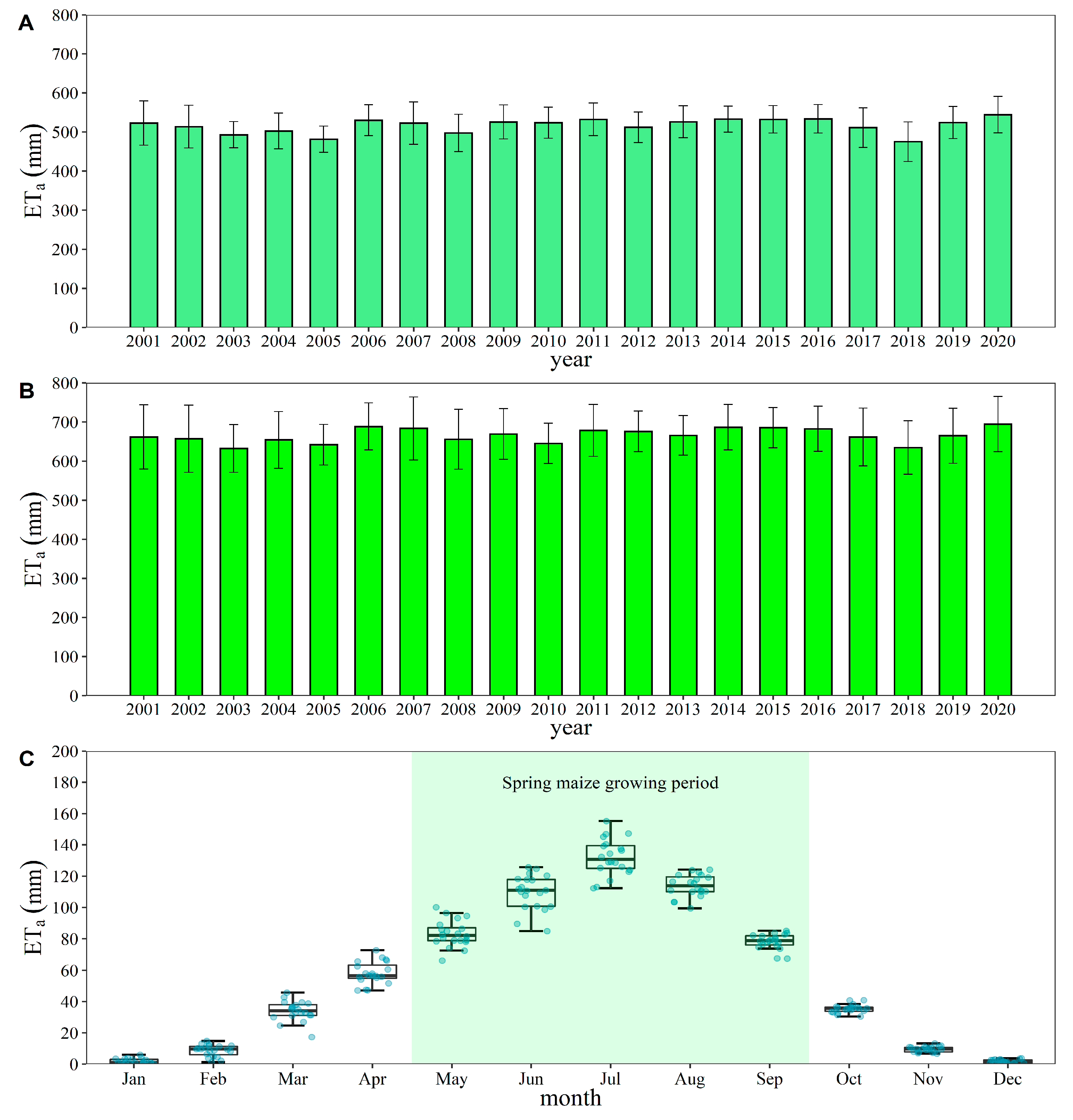
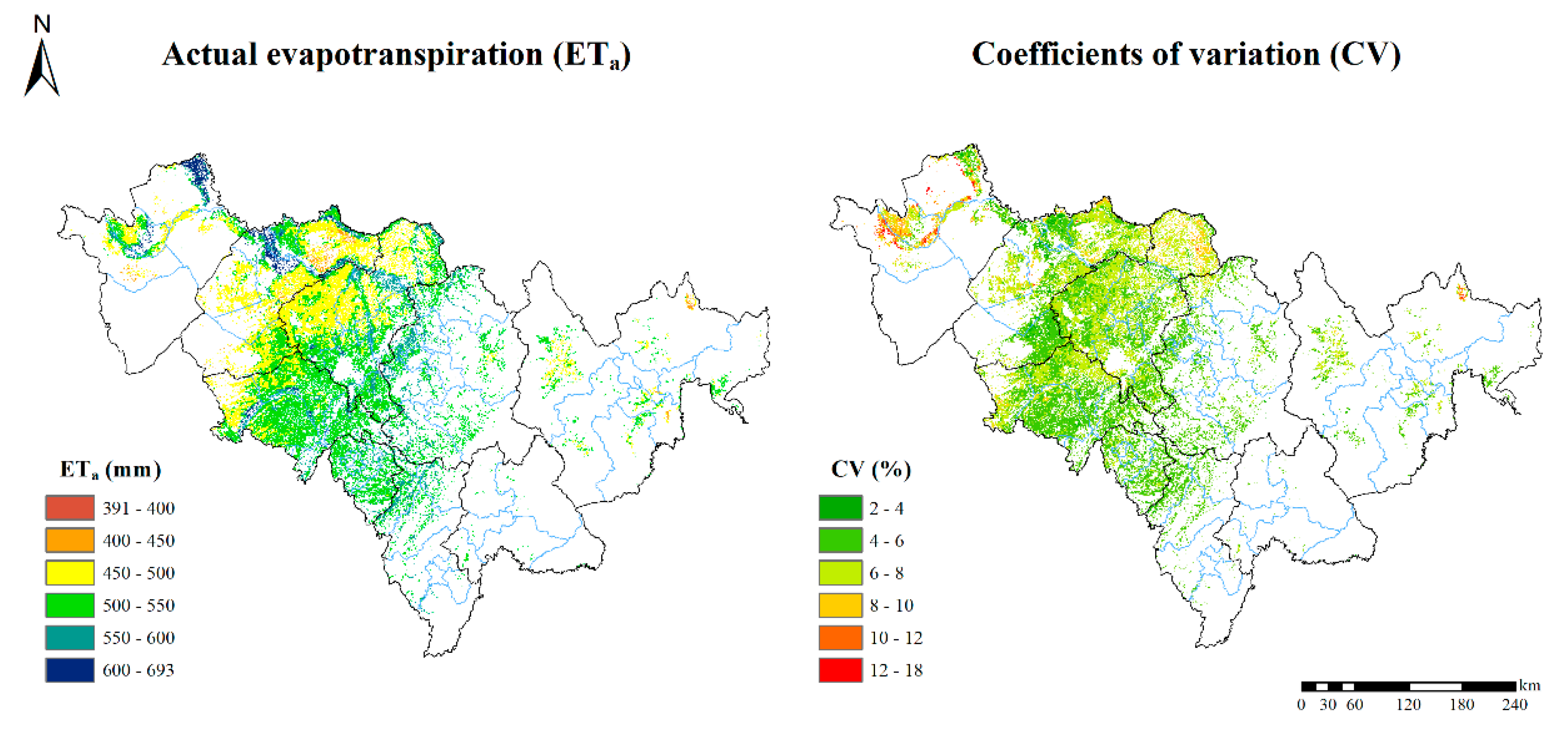
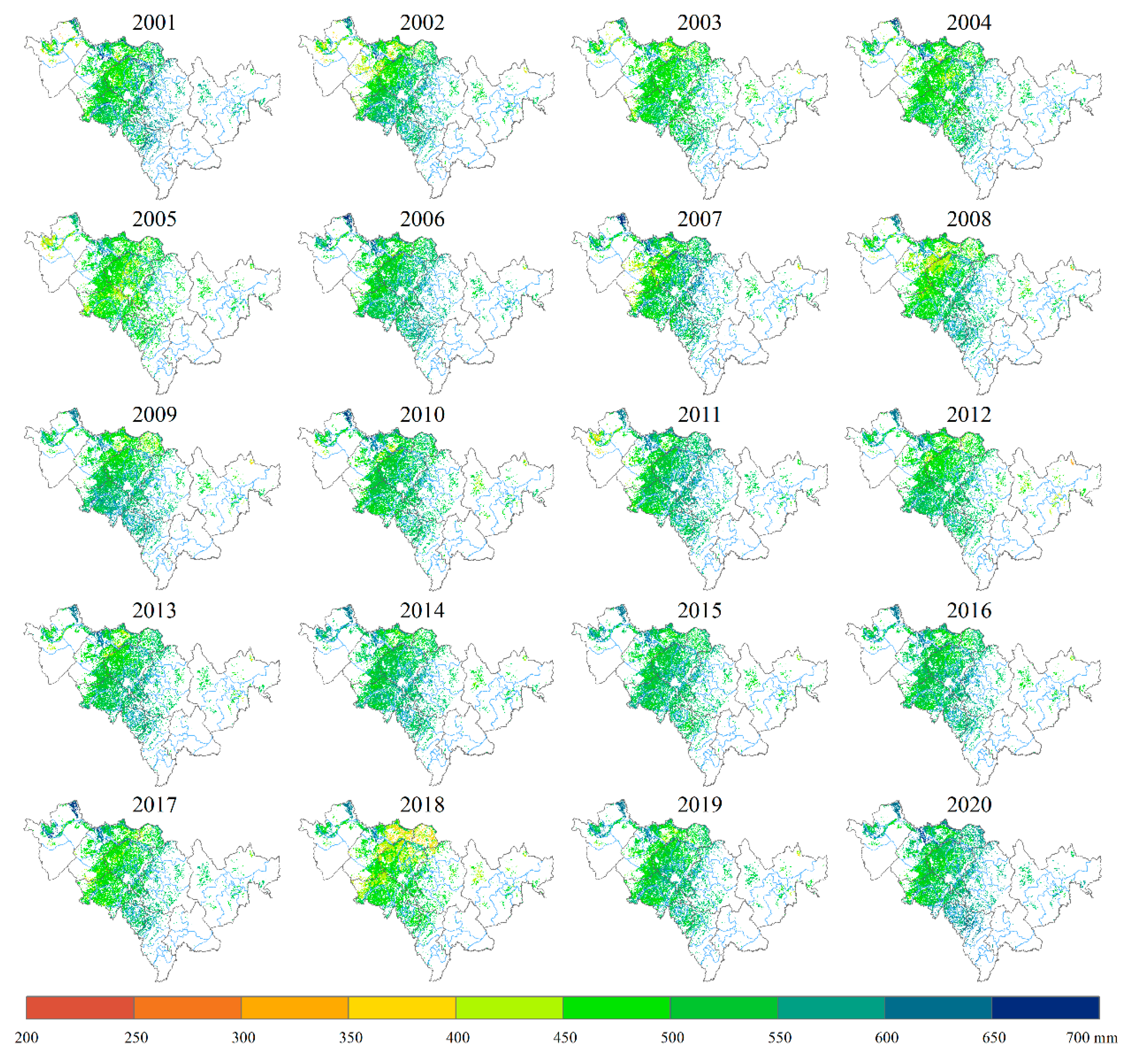
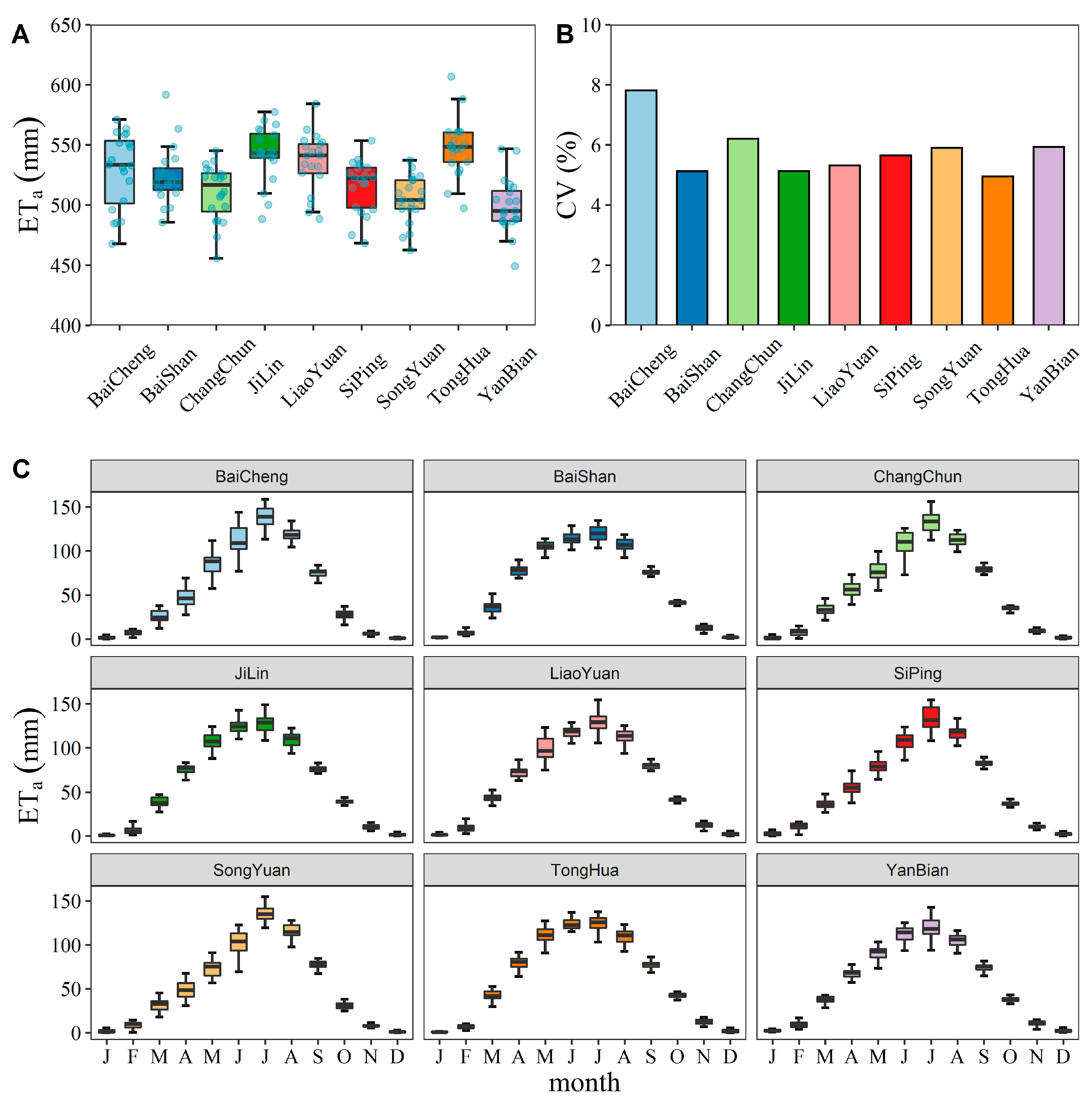
3.2. Temporal and Spatial Distribution Patterns of ETa

The temporal distribution pattern of ETa during the spring maize growing period (May to September) from 2001 to 2020 in Jilin Province is shown in Figure 11. The average cumulative ETa during the growing period of spring maize in Jilin Province ranged from 475 to 544 mm, with a multi-year average value of 517 mm and an average standard deviation value of 43 mm (Figure 11A). The lowest and highest ETa happened in 2008 and 2020, respectively. The average annual cumulative ETa differed from 632 to 694 mm, with a mean value of 666 mm, and the standard deviation varied from 50 to 86 mm, with a mean value of 65 mm (Figure 11B). The monthly distribution pattern of ETa showed a trend of increasing and then decreasing, with the monthly average ETa of 2, 9, 34, 58, 83, 110, 132, 114, 78, 35, 9, and 2 mm from January to December, respectively, with the highest value of ETa in July. The cumulative ETa was 517 mm from May to September during the spring maize growing period (Figure 11C).
The spatial distribution of the multi-year average ETa and inter-annual coefficient of variation (CV) of spring maize in Jilin Province from 2001 to 2020 is shown in Figure 12. The multi-year average ETa was between 391 and 693 mm in Jilin Province, and the multi-year average ETa in Changchun City, Siping City, Jilin City, Liaoyuan City, and other regions was between 450 and 550 mm. Farmland near rivers, such as the Dongliao River in Siping City, the Songhua River across Songyuan City and Changchun City, and the Nen River across the border of Baicheng City, had the ETa above 600 mm. Areas with annual average ETa less than 450 mm were mainly distributed in the western region of Jilin Province, such as Baicheng City, Songyuan City, and the eastern part of Siping City. This might be because these areas had mostly sandy soil and insufficient rainfall. The CV of the multi-year average ETa of spring maize was mostly between 2% and 18% in Jilin Province. In a few areas, such as the western part of Baicheng City and Songyuan City, the inter-annual CV exceeded 10%, which might be caused by the large variation in inter-annual rainfall in these areas. Figure 13 shows the distribution of ETa during the growing season of spring maize in Jilin Province in all years: the ETa was lower in 2005, 2008, and 2018 compared to other years, and the ETa in the rest of the years was relatively stable and maintained between 450 and 550 mm.
The ETa values for each city in Jilin Province are shown in Figure 14. ETa for the spring maize growing season in each city basically remained between 450–550 mm from 2001 to 2020, and the largest multi-year average ETa was in Tonghua, Jilin, and Liaoyuan with ETa exceeded 530 mm. The smallest ETa was in Yanbian, Songyuan, and Changchun with an ETa lower than 510 mm (Figure 14A). The CV of ETa for the spring maize growing season in each city ranged from 5% to 8%, with the smallest variability being 5% in Tonghua and the largest variability being 7.8% in Baicheng (Figure 14B). The distribution of ETa by month in each city is shown in Figure 14C. ETa was mainly concentrated in May–September, i.e., during the growing period of spring maize, and reached its maximum in July with an average of approximately 150 mm.

4. Discussion

4.1. Comparison of the Calculated ETa Results with Similar Studies

To verify the rationality of the ETa calculation results, this study has gathered and sorted out related studies for comparison (Table 2). Guo et al. [47] estimated the ETa of spring maize in Yushu City, Jilin Province, in 2013, using a large weighing lysimeter on a farm scale, and found an average value of 362 mm for ETa. Qiu et al. [48] and Zhang et al. [49] used the Penman–Monteith and crop coefficient method to estimate the 3-year and 54-year ETa of spring maize in Jilin Province, and the average values were 523 mm and 538 mm, respectively, which were similar to the results of this study. Liu [50] used the SIMETAW (Simulation Evapotranspiration of Applied Water) model to simulate the evapotranspiration of the spring maize growing season under different hydrological year types in western Liaoning from 2007 to 2009, and the results were 464 mm, 485 mm, and 486 mm in abundant, flat, and dry years, respectively.
In this study, the ETa values of spring maize in Jilin Province from 2001 to 2020 were between 391 mm and 693 mm, with a multi-year average of 517 mm. This was similar to the results of other related studies in Jilin Province. Jiang et al. [51] pointed out that the maximum error value of ETa estimated by using remote sensing data is reasonable within ±20%. However, Seguin et al. [52] suggested that the maximum error of ETa estimated by remote sensing changes with the actual applications, and the absolute value is usually reasonable around 15–30%. Since there is no relevant flux tower data in the study area that can be used directly for the validation of this model for ETa estimations, a relevant literature review was conducted to validate the estimation effectiveness of this PySEBS model on ETa in Jilin Province. The results of relevant literature studies on spring maize ETa in Jilin Province at the regional scale were 514 mm on average, while the average result of the PySEBS model was 517 mm, with a relative error of less than 1%, indicating a good applicability of the modified model in regional studies (Table 2).
PySEBS software has a high application value in water use evaluation and irrigation management. Based on this model, Ren et al. [30] studied the spatio-temporal patterns of water consumption and irrigation demand during winter wheat-summer maize agricultural production in the Huang-Huai-Hai Plain (3HP), and the scenario analysis of different cropping methods was evaluated. The annual average ETa of winter wheat-summer maize ranged from 700–900 mm with no significant change, while irrigation water demand showed a large interannual variation. In addition, four alternatives that may require less irrigation were tested, i.e., wheat-maize-wheat-fallow (WMWF), wheat-maize-fallow-maize (WMFM), wheat-maize-fallow-spring maize (WMFSM), and fallow-spring maize-fallow-spring maize (FSMFSM), with the results showing that FSMFSM has the best water savings, reducing irrigation by 64%.

4.2. Advantages and Disadvantages of PySEBS Software

Before the development of PySEBS software, studies were conducted by calculating regional ETa using the SEBS module embedded in ILWIS software (https://52north.org/software/software-projects/ilwis (accessed on 1 April 2019)), but the SEBS module has many shortcomings, such as a tedious calculation process, inefficient calculation, only one period of results can be calculated at one time, a lack of batch processing capability, and various coefficient transformations of data are required during processing to make the data into integer form for further operations, which is more challenging for beginners who need to calculate ETa products urgently, and unfavorable for ETa estimation at a large spatial and temporal scales.
To overcome the aforementioned disadvantages, this study developed a more user-friendly PySEBS, which has the following advantages compared with the conventional calculation method. The strengths are to (1) simplify the preprocessing process of remote sensing data and meteorological data, especially meteorological data can be directly interpolated from point-scale data to raster files; (2) develop a concise user interface that makes the input and output of data and modification of parameters more straightforward and convenient; and (3) reduce the time consumption greatly. Once the required parameters are set, the whole process will no longer require the users to manually input data year by year, and the ETa results can be calculated automatically and continuously for many years on a regional scale. In addition, the newly developed PySEBS model can be used to calculate crop water productivity [30], which is very useful for land degradation assessment [53].
Although the PySEBS model performed relatively well in this study, there were some limitations: since the cover type primarily targeted in this study was spring maize, the calculations of ETa in estimating other crops might be inadequate; another point is that the spatial and temporal resolutions of the remote sensing data used need to be further improved, and the spatial resolution of 500–1000 m is not sufficient to distinguish the evapotranspiration characteristics in areas with complex surface cover types, and the existence of mixed image elements may affect the estimation results to a certain extent. Finally, users can also use remote sensing data from other sources, such as Landsat and Sentinel satellites, rather than being limited to MODIS remote sensing data. However, some of the relevant equations in the Supplementary Materials, for example, Equation (3) for calculating surface albedo needs to be adjusted accordingly. Future research should pay more attention to the estimation of evapotranspiration on different surface cover types and the selection of remote sensing data with a higher resolution.

5. Conclusions

A scientific calculation software named PySEBS was developed to calculate ETa on a regional scale. Its most important feature is that it can preprocess remote sensing data and meteorological data quickly, efficiently, and continuously, and calculate the regional ETa on a daily basis. Detailed descriptions of the installation environment, input data requirements, selection method of meteorological data interpolation, formula sources and derivations, and operation procedures of the PySEBS software are presented in this study, which walk the users through the whole set-up and help them to understand the software principles. In addition, spring maize in Jilin Province was selected as the research object, and ETa was calculated during the growing season of spring maize from 2001 to 2020. Finally, the spatio-temporal distribution patterns of ETa during the growing season of spring maize in Jilin Province were mapped and analyzed in this study.
Results indicated that the multi-year average extraction accuracy of the spring maize planting area was 90.6% and that the overall R2 between the statistical area of spring maize and the extracted area in all years was 0.81. The average cumulative ETa of spring maize in the growing season in Jilin Province from 2001 to 2020 ranged from 475 to 544 mm, with a multi-year mean of 517 mm and a standard deviation mean of 43 mm. The highest ETa was in July with a mean of 132 mm. On the spatial scale, the multi-year mean ETa ranged from 391 to 693 mm, and the CV was mostly between 2% and 18%. The cities with the largest multi-year average ETa values were Tonghua, Jilin, and Liaoyuan, and all of them had ETa over 530 mm. The multi-year average ETa of spring maize growing season in Jilin Province in this study was 517 mm, which was similar to the results of other related studies in Jilin Province, and the values were within a reasonable range, indicating that the PySEBS software could estimate the ETa values well. Therefore, PySEBS software can have useful applications in the spatio-temporal patterns of water consumption and irrigation demand in regional scales and associated water saving scenarios.

Supplementary Materials

The following supporting information can be downloaded at: https://www.mdpi.com/article/10.3390/rs14215629/s1, PySEBS V1.0.0 Actual Evapotranspiration (ETa) Calculator User’s Guide [7,18,31,32,33,34,35,36,37,38,39,40,41,42].

Author Contributions

Conceptualization, H.L. and Y.C.; methodology, H.L. and Y.C.; software, H.L. and P.R.; validation, H.L. and Y.C.; formal analysis, H.L. and Y.C.; investigation, H.L.; resources, F.H. and Y.C.; data curation, F.H.; writing—original draft preparation, H.L., Y.C. and Y.L.; writing—review and editing, H.L., Y.C., Y.L., G.W.M. and B.D.; visualization, H.L.; supervision, Y.C., B.L. and F.H.; project administration, B.L. and Y.C.; funding acquisition, Y.C. and F.H. All authors have read and agreed to the published version of the manuscript.

Funding

This research was funded by the Chinese Universities Scientific Fund under award numbers 1191-15051002, 1191-10092004, 1191-15052008, and 1191-31051204. The study was also supported by the National Key Research and Development Program of China under grant numbers 2016YFD0300801 and 2016YFD0300801013.

Institutional Review Board Statement

Not applicable.

Informed Consent Statement

Not applicable.

Data Availability Statement

PySEBS software and 2019 case data are freely distributed through a GitHub public repository (https://github.com/haipengliuCAU/PySEBS, accessed on 15 August 2022).

Acknowledgments

We thank the National Aeronautics and Space Administration (NASA) and the National Meteorological Information Center (NMIC) for providing the MODIS remote sensing data and meteorological data. We greatly appreciate four anonymous reviewers for their valuable comments and suggestions for improving this article.

Conflicts of Interest

The authors declare no conflict of interest.

References

  1. Peng, L.Q.; Zeng, Z.Z.; Wei, Z.W.; Chen, A.P.; Wood, E.F.; Sheffield, J. Determinants of the ratio of actual to potential evapotranspiration. Glob. Change Biol. 2019, 25, 1326–1343. [Google Scholar] [CrossRef] [PubMed] [Green Version]
  2. Tasumi, M. Estimating evapotranspiration using METRIC model and Landsat data for better understandings of regional hydrology in the western Urmia Lake Basin. Agric. Water Manag. 2019, 226, 105805. [Google Scholar] [CrossRef]
  3. McMahon, T.A.; Peel, M.C.; Lowe, L.; Srikanthan, R.; McVicar, T.R. Estimating actual, potential, reference crop and pan evaporation using standard meteorological data: A pragmatic synthesis. Hydrol. Earth Syst. Sci. 2013, 17, 1331–1363. [Google Scholar] [CrossRef] [Green Version]
  4. Xiang, K.Y.; Li, Y.; Horton, R.; Feng, H. Similarity and difference of potential evapotranspiration and reference crop evapotranspiration—A review. Agric. Water Manag. 2020, 232, 106043. [Google Scholar] [CrossRef]
  5. Gutierrez-Ninahuaman, C.; Gonzalez-Herrera, R. Software to analyze ETo. Compilation of indirect methods. Environ. Model. Softw. 2021, 142, 105056. [Google Scholar] [CrossRef]
  6. Dingman, S.L. Physical Hydrology, 1st ed.; Prentice Hall: Hoboken, NJ, USA, 1992. [Google Scholar]
  7. Allen, R.G.; Pereira, L.S.; Raes, D.; Smith, M. Crop Evapotranspiration—Guidelines for Computing Crop Water Requirements—FAO Irrigation and Drainage Paper 56; FAO: Rome, Italy, 1998. [Google Scholar]
  8. Bowen, I.S. The ratio of heat losses by conduction and by evaporation from any water surface. Phys. Rev. 1926, 27, 779–787. [Google Scholar] [CrossRef] [Green Version]
  9. Thornthwaite, C.W.; Holzman, B. The determination of evaporation from land and water surfaces. Mon. Weather Rev. 1939, 67, 4–11. [Google Scholar] [CrossRef]
  10. Penman, H.L. Natural evaporation from open water, bare soil and grass. Proc. R. Soc. Lond. Ser. A 1948, 193, 120–145. [Google Scholar] [CrossRef]
  11. Monteith, J.L. Evaporation and environment. Symp. Soc. Exp. Biol. 1965, 19, 205–234. [Google Scholar]
  12. Shuttleworth, W.J.; Wallace, J.S. Evaporation from sparse crops-an energy combination theory. Q. J. R. Meteorol. Soc. 1985, 111, 839–855. [Google Scholar] [CrossRef]
  13. Dolman, A.J. A multiple-source land surface energy balance model for use in general circulation models. Agric. For. Meteorol. 1993, 65, 21–45. [Google Scholar] [CrossRef]
  14. Choudhury, B.J.; Monteith, J.L. A four-layer model for the heat budget of homogeneous land surfaces. Q. J. R. Meteorol. Soc. 2010, 114, 373–398. [Google Scholar] [CrossRef]
  15. Norman, J.M.; Kustas, W.P.; Humes, K.S. Source approach for estimating soil and vegetation energy fluxes in observations of directional radiometric surface temperature. Agric. For. Meteorol. 1995, 77, 263–293. [Google Scholar] [CrossRef]
  16. Carlson, T. An overview of the "triangle method" for estimating surface evapotranspiration and soil moisture from satellite imagery. Sensors 2007, 7, 1612–1629. [Google Scholar] [CrossRef] [Green Version]
  17. Bastiaanssen, W.G.M.; Menenti, M.; Feddes, R.A.; Holtslag, A.A.M. A remote sensing surface energy balance algorithm for land (SEBAL)—1. Formulation. J. Hydrol. 1998, 212, 198–212. [Google Scholar] [CrossRef]
  18. Su, Z. The Surface Energy Balance System (SEBS) for estimation of turbulent heat fluxes. Hydrol. Earth Syst. Sci. 2002, 6, 85–99. [Google Scholar] [CrossRef]
  19. Allen, R.G.; Tasumi, M.; Trezza, R. Satellite-based energy balance for mapping evapotranspiration with internalized calibration (METRIC)—Model. J. Irrig. Drain. Eng. ASCE 2007, 133, 380–394. [Google Scholar] [CrossRef]
  20. Long, D.; Singh, V.P. A Two-source Trapezoid Model for Evapotranspiration (TTME) from satellite imagery. Remote Sens. Environ. 2012, 121, 370–388. [Google Scholar] [CrossRef]
  21. Laipelt, L.; Kayser, R.H.B.; Fleischmann, A.S.; Ruhoff, A.; Bastiaanssen, W.; Erickson, T.A.; Melton, F. Long-term monitoring of evapotranspiration using the SEBAL algorithm and Google Earth Engine cloud computing. ISPRS J. Photogramm. Remote Sens. 2021, 178, 81–96. [Google Scholar] [CrossRef]
  22. Du, J.; Song, K.S.; Wang, Z.M. Estimation of water consumption and productivity for rice through integrating remote sensing and census data in the Songnen Plain, China. Paddy Water Environ. 2015, 13, 91–99. [Google Scholar] [CrossRef]
  23. Bhattarai, N.; Liu, T. LandMOD ET mapper: A new matlab-based graphical user interface (GUI) for automated implementation of SEBAL and METRIC models in thermal imagery. Environ. Model. Softw. 2019, 118, 76–82. [Google Scholar] [CrossRef]
  24. Mhawej, M.; Faour, G. Open-source Google Earth Engine 30-m evapotranspiration rates retrieval: The SEBALIGEE system. Environ. Model. Softw. 2020, 133, 104845. [Google Scholar] [CrossRef]
  25. Ramirez-Cuesta, J.M.; Allen, R.G.; Intrigliolo, D.S.; Kilic, A.; Robison, C.W.; Trezza, R.; Santos, C.; Lorite, I.J. METRIC-GIS: An advanced energy balance model for computing crop evapotranspiration in a GIS environment. Environ. Model. Softw. 2020, 131, 104770. [Google Scholar] [CrossRef]
  26. Ellsasser, F.; Roll, A.; Stiegler, C.; Hendrayanto; Hölscher, D. Introducing QWaterModel, a QGIS plugin for predicting evapotranspiration from land surface temperatures. Environ. Model. Softw. 2020, 130, 104739. [Google Scholar] [CrossRef]
  27. Wu, F.; Wu, B.; Zhu, W.; Yan, N.; Ma, Z.; Wang, L.; Lu, Y.; Xu, J. ETWatch cloud: APIs for regional actual evapotranspiration data generation. Environ. Model. Softw. 2021, 145, 105174. [Google Scholar] [CrossRef]
  28. Kayser, R.H.; Ruhoff, A.; Laipelt, L.; Kich, E.D.; Roberti, D.R.; Souza, V.D.; Rubert, G.C.D.; Collischonn, W.; Neale, C.M.U. Assessing geeSEBAL automated calibration and meteorological reanalysis uncertainties to estimate evapotranspiration in subtropical humid climates. Agric. For. Meteorol. 2022, 314, 108775. [Google Scholar] [CrossRef]
  29. Huang, C.L.; Li, Y.; Gu, J.; Lu, L.; Li, X. Improving estimation of evapotranspiration under water-limited conditions based on SEBS and MODIS data in arid regions. Remote Sens. 2015, 7, 16795–16814. [Google Scholar] [CrossRef] [Green Version]
  30. Ren, P.P.; Huang, F.; Li, B.G. Spatiotemporal patterns of water consumption and irrigation requirements of wheat-maize in the Huang-Huai-Hai Plain, China and options of their reduction. Agric. Water Manag. 2022, 263, 107468. [Google Scholar] [CrossRef]
  31. Han, X.P.; Wang, Y.Q.; Bao, L. Introduction of ILWIS functions and its scanning digital application. Lab. Sci. 2008, 2, 107–109. [Google Scholar] [CrossRef]
  32. Liang, S.L. Narrowband to broadband conversions of land surface albedo I Algorithms. Remote Sens. Environ. 2001, 76, 213–238. [Google Scholar] [CrossRef]
  33. Yang, X.T. Evapotranspiration Estimating using Remote Sensing and Spatial-Temporal Distribution of Evapotranspiration in Golmud River Basin Based on SEBS Model. Master’s Thesis, Chang’an University, Xi’an, China, 2017. [Google Scholar]
  34. Wu, Y.L. Research on Retrieving and Spatial-Temporal Changes of Evaporation Estimation in the Yellow River Delta Based on Refined SEBS Model. Master’s Thesis, China University of Petroleum, Beijing, China, 2010. [Google Scholar]
  35. Li, X. Estimation of Sensible Heat Flux Based on SEBS Model and Its Application for Drought Monitoring. Master’s Thesis, Nanjing University of Information Engineering, Nanjing, China, 2012. [Google Scholar]
  36. Hao, J.W. Study on Evapotranspiration Based on SEBS Model in Handan. Master’s Thesis, Hebei University of Engineering, Handan, China, 2018. [Google Scholar]
  37. Jobson; Harvey, E. Evaporation into the atmosphere: Theory, history, and applications. Eos Trans. Am. Geophys. Union 1982, 63, 1223. [Google Scholar] [CrossRef]
  38. Hogstrom, U. Non-dimensional wind and temperature profiles in the atmospheric surface layer: A re-evaluation. Bound. Layer Meteor. 1988, 42, 55–78. [Google Scholar] [CrossRef]
  39. Kader, B.A.; Yaglom, A.M. Mean fields and fluctuation moments in unstably stratified turbulent boundary layers. J. Fluid Mech. 1990, 212, 637–662. [Google Scholar] [CrossRef]
  40. Beljaars, A.C.M.; Holtslag, A.A.M. Flux parameterization over land surfaces for atmospheric models. J. Appl. Meteorol. 1991, 30, 327–341. [Google Scholar] [CrossRef]
  41. VandenHurk, B.; Holtslag, A.A.M. On the bulk parameterization of surface fluxes for various conditions and parameter ranges. Bound. Layer Meteor. 1997, 82, 119–134. [Google Scholar] [CrossRef]
  42. Brutsaert, W. Aspects of bulk atmospheric boundary layer similarity under free-convective conditions. Rev. Geophys. 1999, 37, 439–451. [Google Scholar] [CrossRef]
  43. Shuttleworth, W.J. FIFE: The variation in energy partition at surface flux sites. IAHS 1989, 186, 67–74. [Google Scholar]
  44. Sugita, M.; Brutsaert, W. Daily evaporation over a region from lower boundary layer profiles measured with radiosondes. Water Resour. Res. 1991, 27, 747–752. [Google Scholar] [CrossRef]
  45. Crago, R.D. Comparison of the evaporative fraction and the Priestley-Taylor alpha for parameterizing daytime evaporation. Water Resour. Res. 1996, 32, 1403–1409. [Google Scholar] [CrossRef]
  46. Li, G. Estimation Evapotranspiration in Yingtan Agricultural Watershed using SEBAL and SEBS Model. Master’s Thesis, Nanjing University of Information Engineering, Nanjing, China, 2014. [Google Scholar]
  47. Guo, C.M.; Ren, J.Q.; Zhang, T.L.; Yu, H. Dynamic change of evapotranspiration and influenced factors in the spring maize field in Northeast China. Chin. J. Agrometeorol. 2016, 37, 400–407. [Google Scholar] [CrossRef]
  48. Qiu, M.J.; Guo, C.M.; Wang, D.N.; Yuan, F.X.; Qu, S.M.; Ren, J.Q.; Li, Z.H.; Mu, J. Variation of effective precipitation and water deficit index in maize growing season in Jilin Province during 1960–2015. Agric. Res. Arid. Reg. 2018, 36, 237–280. [Google Scholar] [CrossRef]
  49. Zhang, Y.; Wang, L.X.; Li, Q.; Hu, Z.H.; Guo, C.M.; Ren, J.Q. Irrigation simulation of spring maize in central and western of Jilin Province based on WOFOST model. Chin. J. Agrometeorol. 2018, 39, 411–420. [Google Scholar] [CrossRef]
  50. Liu, Y. Simulation and Applications of Maize Evapotranspiration Based on SIMETAW Model. Master’s Thesis, Chinese Academy of Agricultural Sciences, Beijing, China, 2011. [Google Scholar]
  51. Jiang, H.; Liu, S.R.; Sun, P.S.; An, S.Q.; Zhou, G.Y.; Li, C.Y.; Wang, J.X.; Yu, H.; Tian, X.J. The influence of vegetation type on the hydrological process at the landscape scale. Can. J. Remote Sens. 2004, 30, 743–763. [Google Scholar] [CrossRef] [Green Version]
  52. Seguin, B.; Becker, F.; Phulpin, T.; Gu, X.F.; Guyot, G.; Kerr, Y.; King, C.; Lagouarde, J.P.; Ottle, C.; Stoll, M.P. IRSUTE: A minisatellite project for land surface heat flux estimation from field to regional scale. Remote Sens. Environ. 1999, 68, 357–369. [Google Scholar] [CrossRef]
  53. Schillaci, C.; Jones, A.; Vieira, D.; Munafò, M.; Montanarella, L. Evaluation of the United Nations sustainable development goal 15.3.1 indicator of land degradation in the European Union. Land Degrad. Dev. 2022, 1–19. [Google Scholar] [CrossRef]
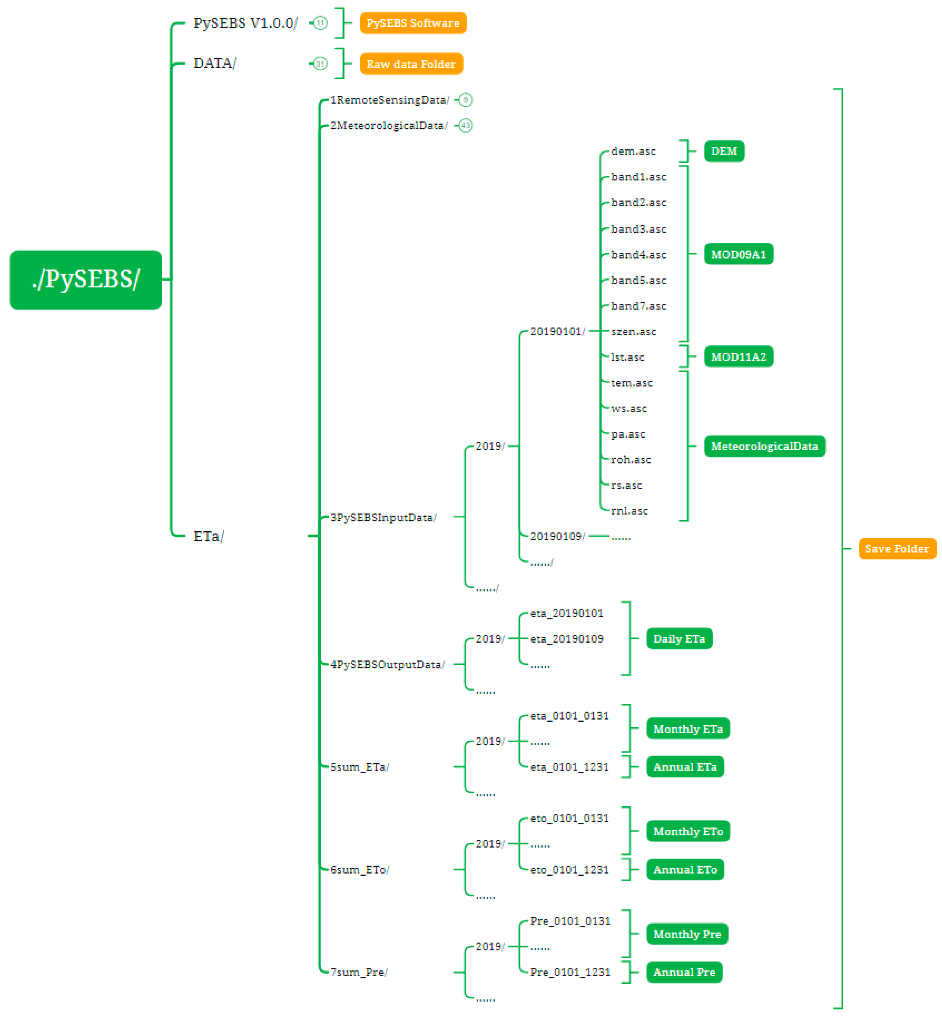
Figure 1. Schematic diagram of the PySEBS software file structure.
Remotesensing 14 05629 g001
Figure 2. Graphical user interface of PySEBS software. The upper left part is the main menu, the upper right part is the module 1-remote sensing data processing; the lower left part is the module 2-meteorological data processing; and the lower right part is the module 3-PySEBS calculation and processing.
Remotesensing 14 05629 g002
Figure 3. Structure of the path to the initial input data.
Remotesensing 14 05629 g003
Figure 4. Schematic diagram of the structure of folder 1RemoteSensingData/ and folder 2MeteorologicalData/.
Remotesensing 14 05629 g004
Figure 5. The example format of the meteorological data in replacement for the V3.0 data in 1RawData/.
Remotesensing 14 05629 g005
Figure 6. Schematic diagram of the structure of folders 3PySEBSInputData/, 4PySEBSOutputData/, and 5sum_ETa/, 6sum_ETo/, and 7sum_Pre/.
Remotesensing 14 05629 g006
Figure 7. Location of the study area, sampling sites for extraction of planting area, and DEM map.
Remotesensing 14 05629 g007
Figure 8. Comparison of before and after MODIS-NDVI time series reconstruction of spring maize.
Remotesensing 14 05629 g008
Figure 9. Schematic map of decision tree classification extraction for spring maize planting area.
Remotesensing 14 05629 g009
Figure 10. Results of planting area extraction for spring maize.
Remotesensing 14 05629 g010
Figure 11. Temporal distribution pattern of ETa of spring maize in Jilin Province from 2001 to 2020. (A) Cumulative ETa during the spring maize growing periods for all years (1 May to 30 September); (B) cumulative ETa throughout the year in the spring maize growing area for all years (1 January to 31 December); (C) monthly distribution of ETa over the spring maize growing area for 20 years, where the shaded part represents the spring maize growing period. Data are presented as mean plus or minus standard deviation.
Remotesensing 14 05629 g011
Figure 12. Multi-year average ETa (2001–2020) and its coefficient of variation (CV) during the growing period of spring maize in Jilin Province.
Remotesensing 14 05629 g012
Figure 13. ETa of spring maize during growing season over the years.
Remotesensing 14 05629 g013
Figure 14. ETa of spring maize in each city of Jilin Province. (A) Multi-year average ETa in each city during the spring maize growing season from 2001 to 2020, (B) coefficient of variation (CV) of ETa during the spring maize growing season in each city from 2001 to 2020, and (C) monthly ETa in each city.
Remotesensing 14 05629 g014
Table 1. Basic information on MODIS products.
ProductsSurface Characteristics ParametersTemporal ResolutionSpatial Resolution
MOD09A1Surface albedo (Band 1–7)
Solar zenith angle (Szen)
8 d500 m
MOD11A2Surface temperature (lst)8 d1000 m
Table 2. Comparison of the PySEBS estimated spring maize ETa with similar studies (unit: mm).
Study MethodScaleCropValue RangeMeanPeriodAreaSource
Weighting lysimeterFarmlandSpring maize-3622013Yushu City, Jilin ProvinceGuo, [47]
Penman–Monteith + Crop coefficient methodRegionalSpring maize452–6375231981–2014Jilin ProvinceQiu, [48]
Penman–Monteith + Crop coefficient methodRegionalSpring maize455–6415381961–2015Midwest Jilin ProvinceZhang, [49]
SIMETAW ModelRegionalSpring maize464–4864802007–2009Fuxin, Liaoning ProvinceLiu, [50]
PySEBS ModelRegionalSpring maize391–6935172000–2017Jilin ProvinceThis study
Publisher’s Note: MDPI stays neutral with regard to jurisdictional claims in published maps and institutional affiliations.

