Abstract
Soil salinization is one of the major degradation processes threatening food security and sustainable development. Detailed soil salinity information is increasingly needed to tackle this global challenge for improving soil management. Soil-visible and near-infrared (Vis-NIR) spectroscopy has been proven to be a potential solution for estimating soil-salinity-related information (i.e., electrical conductivity, EC) rapidly and cost-effectively. However, previous studies were mainly conducted at the field, regional, or national scale, so the potential application of Vis-NIR spectroscopy at a global scale needs further investigation. Based on an extensive open global soil spectral library (61,486 samples with both EC and Vis-NIR spectra), we compared four spectral predictive models (PLSR, Cubist, Random Forests, and XGBoost) in estimating EC. Our results indicated that XGBoost had the best model performance (R2 of 0.59, RMSE of 1.96 dS m−1) in predicting EC at a global scale, whereas PLSR had a relatively limited ability (R2 of 0.39, RMSE of 2.41 dS m−1). The results also showed that auxiliary environmental covariates (i.e., coordinates, elevation, climatic variables) could greatly improve EC prediction accuracy by the four models, and the XGBoost performed best (R2 of 0.71, RMSE of 1.65 dS m−1). The outcomes of this study provide a valuable reference for improving broad-scale soil salinity prediction by the coupling of the spectroscopic technique and easily obtainable environmental covariates.
1. Introduction
Wide-spread soil salinity is one of the major soil degradations that threaten food security and sustainable development, especially in arid and semi-arid regions. It is estimated that soil salinity impacts areas of more than one billion ha globally under human-induced actions and global climate change [1,2,3]. A recent report stressed that soil salinity takes up to 1.5 million ha of cropland out of production and decreases the potential production of a further 20–46 million ha each year, leading to an annual loss of around US$ 31 million [4]. Under this context, the campaign of World Soil Day 2021 was set to “Halt soil salinization, boost soil productivity” to raise public awareness for maintaining healthy ecosystems, fighting soil salinization, and improving soil health [5]. To tackle this global challenge, up-to-date information on soil salinity is increasingly required for evidence-based decision-making in enhancing soil management [6,7].
Soil salinity has high spatio-temporal heterogeneity on account of natural events and anthropogenic activities, such as floods, drought, and irrigation [3]. Due to the complexity of soil salinization processes, the updated information on salt-affected soils is necessary to enhance our knowledge of the spatial distribution of saline soils. Therefore, numbers of measured samples are required to represent the spatial variability of soil salinity. The conventional assessment of soil salinity involves the electromagnetic measurement of electrical conductivity (EC) or laboratory chemical analysis, which is rather labor-intensive and time-consuming for monitoring soil salinity at a broad scale [8,9,10]. On the basis of the relationship between spectral signal and soil properties, visible near-infrared (Vis-NIR) spectroscopy is a promising technology for monitoring soil information rapidly and cost-effectively [11,12,13]. The applicability of Vis-NIR for soil salinity prediction has been investigated. The spectral response of salinity in soils is the result of vibrational absorption from the crystal structure of the evaporate minerals [14]. Previous studies have shown that the characteristic bands of soil-salinity-related indicators (e.g., NaCl, KCl and MgSO4) are located within the Vis-NIR range [15,16]. This mechanical relationship paves the foundation for soil salinity detection and monitoring by Vis-NIR spectroscopy.
The successful application of Vis-NIR spectroscopy in soil salinity prediction has been reported in the literature. Partial least squares regression (PLSR) was one of the most commonly used methods in predicting soil salinity with Vis-NIR data, especially in the area where the relationships between soil salinity and spectra are linear [17]. In field scale, linear regression may be suitable for predicting soil salinity with spectral data. For example, Weindorf et al. [18] found that penalized spline regression (R2 = 0.74, RMSE = 1.79 dS m−1) had better model performance than support vector machines (SVM) in estimating EC at a field scale in north-eastern Spain. Furthermore, a non-linear model would be preferred where the spatial heterogeneity soil properties are large at a field scale. Wang et al. [19] found that convolutional neural networks (CNN) performed best (R2 = 0.79, RMSE = 9.41 dS m−1) in the prediction of soil salinity at a field scale in northwestern China [19]. At a broader scale, both linear and nonlinear correlation between soil properties and spectral data should be considered as the complicated soil formation processes [20]. Wang et al. [9] found that the Random Forests (RF) model (R2 = 0.93, RMSE = 4.57 dS m−1) performed better than PLSR in EC prediction at a regional scale in northwestern China. Zhang and Huang [21] demonstrated the better performance of soil salinity prediction (R2 = 0.72, RMSE = 0.39 dS m−1) using principal component regression than PLSR at a regional scale in northeastern China. Nawar et al. [22] found that multivariate adaptive regression splines (R2 = 0.81, RMSE = 6.55 dS m−1) performed better than PLSR in a salt-affected area in Egypt. Bokde et al. [23] showed that SVM had better accuracy (R2 = 0.85, RMSE = 4.01 dS m−1) in soil salinity prediction than RF and gradient-boosted tree at a regional scale in central and eastern Iraq. It may be concluded from these cases that machine learning algorithms generally had better model performance than linear models at a regional scale, whereas the most appropriate model might be case-specific. In addition, most of the previous studies have been conducted in a relatively small scale (e.g., field, regional), and it remains unclear whether a global soil spectral library can be used to predict soil salinity with much greater pedo-climatic heterogeneity and under different spectral measuring protocols.
Based on an open global soil spectral library, the objectives of this study are: (1) comparing the spectral predictive ability of soil salinity on a global scale for PLSR, Cubist, SVM, and Random Forests; and (2) evaluating the benefits of auxiliary environmental covariates in improving soil salinity prediction.
2. Materials and Methods
2.1. Soil Database
The soil data used in this study were freely achieved from the Open Soil Spectral Library (OSSL) [24]. A total of 62,051 soil samples with both Vis-NIR spectra and electrical conductivity (EC) were preliminarily selected. In the OSSL, Vis-NIR was recorded from 350 nm to 2500 nm with a spectral resolution of 2 nm. As the OSSL was compiled from different sources (or spectrometers), some Vis-NIR spectra did not fully cover 350–2500 spectral ranges. Considering the low signal-to-noise ratio at the edge of spectra, we only retained the soil samples (62,027) with a spectral range of 450–2450 nm. The number of soil samples was further reduced to 61,486 by removing the ones without coordinates. Figure 1 presents the spatial distribution of soil sampling sites used in this study. It clearly shows that Europe has the highest soil sampling density, followed by North America, which is mainly located in the USA. Other continents have a sparse distribution of soil sampling locations.
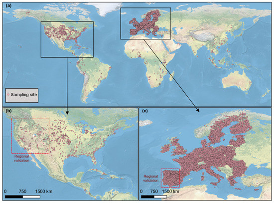
Figure 1.
Spatial distribution of soil sampling sites used in this study. (a) Two areas for the regional validation are located in the western USA (b) and southwestern EU (c).
2.2. Spectral Pre-Processing and Characteristics
Several spectral pre-processing methods, including reflectance (R), absorbance (A), continuum removal (CR), Savitzky–Golay (SG) smoothing, derivative (1st or 2nd order), normal variate transformation (SNV), and their combinations, were conducted for reducing the impaction from the spectral measurement protocols and enhancing the spectral signals. The pre-processing methods were preliminary compared through 5-fold cross-validation using partial least square regression (PLSR). The cross-validation result indicated CR combined with the first derivative SG (polynomial order of 2 and window size of 11) had the lowest prediction error. Therefore, it was selected as the optimal pre-processing method. The spectra were further trimmed to a spectral resolution of 10 nm (198 bands) to reduce multicollinearity without losing accuracy.
The continuum removed reflectance varied under different contents of soil salinity (Figure 2). It displays two deep absorption features around 1415 and 1915 nm, which is relevant to the O–H stretches and the H–O–H bending combination of molecular free water and overtones. Two weak and overlapped absorption features can be found near 2210 and 2385 nm, which are closely related to clay minerals (e.g., kaolinite, gibbsite).
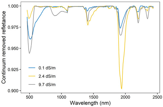
Figure 2.
Continuum removed reflectance of three soil samples at different EC contents.
2.3. Auxiliary Environmental Covariates
A total of seven easily available auxiliary environmental covariates were used in this study.
The coordinates (longitude and latitude) were included to represent the spatial position. The elevation (ELE) data were extracted from the Shuttle Radar Topography Mission (SRTM) data with a spatial resolution of 90 m [25]. The mean annual temperature (MAT) and mean annual precipitation (MAP) were derived from the WorldClim version 2.1 climate data for the years 1970–2000 with a spatial resolution of 1 km [26]. The potential evapotranspiration (PET) and aridity index (AI) were achieved from the Global-PET and Global-Aridity database with a spatial resolution of 1 km [27]. These two global products were both modelled using WorldClim.
2.4. Calibration Methods
In addition to the PLSR model, three machine learning algorithms, namely Cubist, Random Forests (RF), and XGBoost, were used to predict soil EC at a global scale.
PLSR is the most commonly used linear regression model in spectral predictive modelling. It can reduce the spectral dimension and keep the most relevant latent variables by projecting the predictor variables and the response variable to a new space [28]. The number of latent variables (LVs) in PLSR was optimized from 2 to 30 with an interval of 2 by 5-fold cross-validation. Similar to previous studies, PLSR is regarded as a benchmark model in this study [29,30].
Cubist is a piecewise linear decision tree approach developed from the M5 algorithm [31]. It recursively splits the response variables into several subsets, within which the subset has similar predictor variables. These splits are defined by a list of hierarchically ordered rules that have the following format: IF [condition], THEN [linear regression model]; ELSE [go to the next rule]. Once a sample satisfies the condition of one rule, then a relevant linear regression model is used to predict the response variable.
Random Forests is an extension to classification and regression. It consists of multiple trees generated by a combination of bagging and a random selection of predictor variables applied at each split of the trees [32]. The final prediction result is the mean of the outputs of all trees for regression. The RF prediction is stable when the tree number is large enough, and, therefore, we used 500 trees in this study. The number of variables randomly sampled as candidates at each split (mtry) in RF was optimized from 2 to 20 with an interval of 2 by 5-fold cross-validation.
XGBoost is an efficient and scalable implementation of Gradient Boosting Machines (GBM) [33]. The main steps of XGBoost are listed as follows: (1) fit a function that projects predictor variables into a response variable by minimizing the loss function; (2) iteratively fit the regression tree model using the loss function (here, the regression tree model is fitted on the part of the calibration set randomly sampled); (3) merge predictions from all the iterations to get the prediction outcome by multiplying by the weights of regression tree models. Compared to GBM, XGBoost adopts a more regular formalization to control over-fitting. It runs much faster and requires less memory in model fitting, so it is a preferable solution for big data modelling [34,35]. The three most important parameters in XGBoost, namely nrounds (100, 200, 300), max_depth (2, 4, 6), and eta (0.1, 0.2, 0.3), were optimized by 5-fold cross-validation.
All these calibration models were performed with “pls”, “Cubist”, ”ranger”, “xgboost”, and “caret” packages in R [36,37,38,39,40].
2.5. Modelling Strategies
In this study, three modelling strategies were compared: (1) model with full spectra (model_s); (2) model with principal components of spectra (model_pc); and (3) model with principal components of spectra and auxiliary environmental covariates (model_pc_ec). The number of principal components of the spectra was determined at 30, as it explained more than 99% of the variance.
2.6. Model Evaluation
Previous studies indicated that a single random split was comparable to repeated random split and k-fold cross-validation in accuracy and robustness for a large dataset (>1400) [41]. Our preliminary tests on this data were in line with this finding (data not shown). Therefore, this study randomly split the whole dataset into calibration (3/4) and validation (1/4) sets. All the calibration models were evaluated by the same validation set using determination coefficient (R2) and root mean square error (RMSE):
where n is the number of samples, and are measured and predicted values for the sample i, and is the mean of measured values.
In addition to evaluate the model performance at a global scale, we also performed regional validation in western USA and southwestern EU (Figure 1) using the best predictive modelling strategy.
All the calculations were performed in R [40].
3. Results
3.1. Statistical Analysis
Table 1 shows the statistics of the entire, calibration, and validation EC data sets. The minimum and maximum EC were 0.01 and 50 dS m−1, respectively, demonstrating a high heterogeneity. The mean and third quartile of EC were 0.1 and 0.33 dS m−1, and the skewness and kurtosis were 9.84 and 114.17. These statistics indicated that the whole data were dominated by the samples with low EC. According to the soil salinity classification suggested by USDA [42], 94.63% of soil samples were non-saline (0–2 dS m−1), and the proportion of very slightly saline (2–4 dS m−1), slightly saline (4–8 dS m−1), moderately saline (8–16 dS m−1), and strongly saline (>16 dS m−1) were 2.26%, 1.37%, 0.89%, and 0.85%, respectively. The data did not follow a normal distribution, and we kept the original data for modelling, as other transformations did not improve the model performance.

Table 1.
Statistical summary of EC.
3.2. Comparison of Four Algorithms in EC Prediction by Vis-NIR Spectra
Figure 3 represents the performance of four calibration models in predicting EC using full Vis-NIR spectra. The result showed that PLSR had the lowest model performance, with an R2 of 0.39 and RMSE of 2.41 dS m−1. Among the three machine learning algorithms, XGBoost performed best, with an R2 of 0.59 and RMSE of 2.04 dS m−1. All the models showed an underestimation of high EC, especially for the PLSR model.
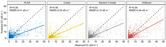
Figure 3.
Scatter plots of four spectral predictive models using full spectra. The solid line is a fitted line for each model, whereas the dashed line is the 1:1 line.
Figure 4 shows the results of four calibration models in predicting EC using the first 30 PCs of Vis-NIR spectra. The model performance of PLSR and Cubist decreased compared to the models with full spectra, whereas RF and XGBoost had rather similar model performance. The XGBoost had the best model performance, with an R2 of 0.59 and RMSE of 1.96 dS m−1, and RF ranked second, with an R2 of 0.57 and RMSE of 2.02 dS m−1.
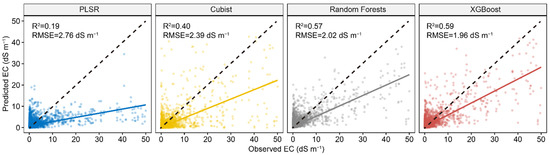
Figure 4.
Scatter plots of four spectral predictive models using first 30 PCs of Vis-NIR spectra. The solid line is a fitted line for each model, whereas the dashed line is the 1:1 line.
3.3. Evaluation of EC Prediction by Vis-NIR Spectra and Environmental Variables
Figure 5 shows the performance comparison among four models using both the first 30 PCs of Vis-NIR and the environmental covariates. The result showed that the PLSR model performed much better than the model with only 30 PCs, but slightly worse than the model with full Vis-NIR spectra. For the three machine learning models, all of them had better performance than models using either full spectra or 30 PCs. The XGBoost model performance best among all the models with R2 of 0.71 and RMSE of 1.65, respectively. Compared to the model with the full spectra, R2 increased 20% and RMSE decreased 19%. The accuracy of RF model was slightly lower than XGBoost, but performed much better than PLSR and Cubist.
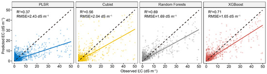
Figure 5.
Scatter plots of four spectral predictive models using first 30 PCs of Vis-NIR spectra and environmental covariates. The solid line is a fitted line for each model, whereas the dashed line is the 1:1 line.
3.4. Variable Importance in EC Prediction
As XGBoost models had the best model performance, we further evaluated their variable importance built on Vis-NIR spectra and environmental variables (Figure 6). The result indicated that spectra were the most important variables for EC prediction, as PC2 and PC1 ranked first and third. Environmental covariates, including elevation, spatial position, and MAP, showed relative importance in the prediction of EC. As shown in Figure 7, the high loadings of PC1 were located around 1400 and 1900 nm, which linked to the overtones of O-H and H-O-H stretch vibrations of free water. The high loadings of PC2 were located at 600, 1450, and 2200 nm, which were correlated to soil organic matter and clay minerals. As for PC7, high loadings occurred around 510, 650, and 2250 nm, relevant to iron oxides and clay lattice.
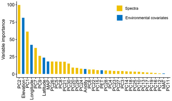
Figure 6.
Variable importance of XGBoost model in EC prediction.
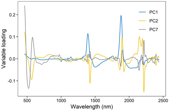
Figure 7.
Variable loading of the three most important principal components (accounting for 85% of total variance) in XGBoost model (PC1, PC2, and PC7).
3.5. Regional Validation
As the XGBoost model using Vis-NIR and auxiliary environmental covariates had the best model performance, it was used to evaluate the model performance at two regions located in the western USA (high-salinity area) and southwestern EU (low-salinity area). The results showed that the global model had a lower model performance in western USA (R2 of 0.45 and RMSE of 2.93 dS m−1) and southwestern EU (R2 of 0.44 and RMSE of 0.21 dS m−1) compared to that at a global scale (R2 of 0.71 and RMSE of 1.65 dS m−1).
4. Discussion
4.1. The Ability of Vis-NIR in EC Prediction at a Global Scale
Our results showed that machine learning models (i.e., Cubist, RF, XGBoost) performed better in EC prediction than PLSR using full Vis-NIR spectra, which is in line with previous findings [43,44,45]. This can be explained by the fact that the relationship between soil salinity and spectral characteristics was non-linear, resulting from the weak overtones and combination bands of functional groups in the Vis-NIR range [15,16]. Machine learning can deal with complex non-linear relationships and, therefore, has become popular in spectral modelling [46]. However, machine learning was weak in extrapolation, so the prediction for samples beyond the validity domain of the machine learning model should be avoided [47,48].
When using the first 30 spectral PCs for EC modelling, PLSR and Cubist decreased in model accuracy, whereas the performances of RF and XGBoost are similar compared to when using the full Vis-NIR spectra. This demonstrated the advantage of RF and XGBoost models: that they can perform well even with fewer variables. This would be crucial for spectral modelling on big data by boosting the modelling efficiency.
Nevertheless, with only spectra as predictors, even the best XGBoost model (R2 = 0.59) still had a lower model performance in EC prediction at a global scale than these reported in previous studies at a smaller scale (R2 = 0.72−0.93) [8,15,16,17]. This may be attributed to the following three aspects:
- (1)
- The quality of spectra varies among different data sources, mainly relating to the difference in spectrometers and spectral measurement protocols [12,49,50]. Though we applied the spectral pre-processing methods to eliminate this effect, the results indicated that this problem was not fully solved.
- (2)
- The investigated scales in previous studies were much smaller than in this study [17,18,19,21,22]. The complex pedo-climatic condition at a global scale leads to a high soil heterogeneity [3,51]; therefore, it poses a greater challenge to predict EC only by soil Vis-NIR spectra compared to previous studies.
- (3)
- The imbalance between non-saline soil (94.63%) and saline soil (5.37%) will lead to the over-presentation of non-saline soil in the predictive model, so the saline soil will have lower accuracy [52].
4.2. The Added Value of Environmental Variables in EC Prediciton
The model performance of EC prediction has been dramatically improved with seven environmental variables into the spectral predictive models. This confirms the benefits of additional environmental variables in improving the spectral model on a global scale. The importance of elevation, MAP, and spatial coordinates has been confirmed in EC prediction. The elevation is highly relevant to the re-distribution of soil salinity via runoff and groundwater depth, as those high-salinity areas are mainly observed in regions with low elevation [53,54]. The MAP has been recognized as a controlling factor in soil salinity by directly influencing the movement of exchangeable base cations along the soil profile. As a result, the areas with a soil salinity threat are mainly located in arid or semi-arid regions with low precipitation. The spatial coordinates are a proxy of the distance between soil sampling sites. This information is useful because the distribution of soil salinity follows the first law of geography that “everything is related to everything else, but near things are more related than distant things” [55].
Our results suggested that PLSR was unsuitable for EC prediction globally due to its weak ability of dealing with complex multivariate linear relations, even with environmental variables. The XGBoost model performed the best; therefore, it is suggested for EC prediction either using spectra only or integrating environmental variables at a broad scale. RF also showed good model performance, but it was always slightly worse than XGBoost. This results from the fact that XGBoost takes an iterative way to combine a series of weak models to create one strong model by addressing the residuals in the prior iterations. This boosting procedure in XGBoost can minimize the residuals so that it generally has a better model performance than RF if the model parameters are well-tuned.
4.3. The Limitations and Perspectives
The majority of the soil samples from the OSSL database are non-saline soil samples, so it is still not representative enough for the arid and semi-arid areas which are suffering from the great threat of soil salinization. However, this limitation can be well addressed in the near future when more countries from these areas join the initiative of OSSL. Additionally, the Global Soil Partnership of FAO established the Global Soil Laboratory Network (GLOSOLAN) to promote the use of soil spectroscopy as a dry chemistry method for more efficient soil analysis. It can be expected that more countries will engage in building their national soil spectral libraries to improve the proficiency of soil laboratories under the standard spectral measuring protocol. Once the soil spectral libraries are representative enough, soil spectroscopy can be a powerful alternative to conventional laboratory analysis worldwide. As shown in Figure 8, the global model may not perform well at a smaller scale, which implies that a regional-specific model can be more helpful in predicting salinity. However, it should be noted that the global OSSL can still be helpful to enhance the regional-specific model by providing a given number of similar soil samples together with memory-based learning [56].
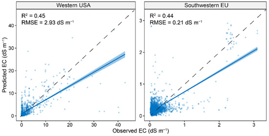
Figure 8.
Scatter plots of predictive models with model performance at two areas for regional validation. The solid line is a fitted line for each model, whereas the dashed line is the 1:1 line.
Another limitation of the OSSL database is that all the soil spectra were collected under different spectral measuring protocols. Though some spectral processing methods (e.g., CR, detrend, smoothing) can alleviate part of the spectral measurement error, the remaining one could still strongly impact the accuracy of calibration models. Therefore, the different soil spectral measurement protocols greatly impede the build-up of broad-scale soil spectral libraries and limit their applications for accurate soil analysis. Though Ben-Dor et al. [57] have been aware of this issue and proposed the standards and protocols for spectral measurements of soils in the laboratory, this is still not fully implemented in practice [58]. Therefore, the methodology for harmonizing the different derived spectral data sets needs to be improved, and future work in soil spectroscopy needs to follow the P4005-Standards and Protocols for Soil Spectroscopy managed by the working group of the IEEE Standards Association (https://sagroups.ieee.org/4005/) (accessed on 13 September 2022).
Laboratory soil spectroscopy is an efficient way for data acquisition and it has a great potential in improving soil salinity monitoring at a broad scale from remote sensing platforms in the following aspects: (1) providing more ground observations for calibrating remote sensing-based models [59,60]; and (2) transferring ground-based soil spectra to remotely sensed spectra of bare soil [61,62,63]. Challenges remain on how to improve the spectral transfer model between ground-based and remotely sensed spectra by accounting for the following effects: (1) disturbance of crop residual, water, and surface roughness on the quality of remotely sensed spectra; (2) mismatch between soil sampling sites and spatial resolution of remote sensing data; (3) identification of the saline soil spectral features combining ground-based spectra and hyperspectral data to predict the spatial distribution of soil salinity across scales; (4) evaluation of the ability of soil spectral predictive model for soil salinity under irrigated and non-irrigated croplands. With more in-depth research focused on filling this knowledge, soil spectroscopic techniques will play a more important role in delivering soil information, so as to maintain soil resources in a sustainable way [64].
5. Conclusions
This study investigated the power of the open soil Vis-NIR spectral library for EC prediction at a global scale. The results showed that the XGBoost model had the best performance when using Vis-NIR spectra, with an R2 of 0.59 and RMSE of 1.96 dS m−1. This model accuracy was slightly lower than previous studies conducted from field to regional scales due to the greater heterogeneity of the pedo-climatic condition and the inconsistency of spectral data sources in this study. Our results confirmed the value of additional auxiliary environmental covariates in improving EC prediction by increasing R2 to 0.71 and decreasing RMSE to 1.65 dS m−1 for the XGBoost model. It can be expected that open soil spectral library will make a greater contribution of efficient soil monitoring when more countries engage in the buildup of this soil spectral library and an international standard of spectral measurement protocol is adopted.
Author Contributions
Conceptualization, Y.Z. and S.C.; methodology, Y.Z.; software, Y.Z.; validation, B.H., W.J., S.L., Y.H., H.X., N.W., J.X., X.Z., Y.X. and Z.S.; formal analysis, Y.Z. and S.C.; writing—original draft preparation, Y.Z. and S.C.; writing—review and editing, B.H., W.J., S.L., Y.H., H.X., N.W., J.X., X.Z., Y.X. and Z.S.; visualization, Y.Z.; supervision, S.C.; funding acquisition, Y.Z. and B.H. All authors have read and agreed to the published version of the manuscript.
Funding
This research was funded by the National Science Foundation of China (grant no. 42001047), the Project of Department of Education Science and Technology of Jiangxi Province (grant no. GJJ210541), and the Social Science Foundation of Jiangxi Province (grant no. 21YJ43D).
Data Availability Statement
The data used in this study was freely obtained from Open Soil Spectral Library, https://doi.org/10.5281/zenodo.5759693, accessed on 19 August 2022.
Acknowledgments
We would like to acknowledge two anonymous reviewers and the academic editor for providing helpful suggestions, which significantly improved our manuscript.
Conflicts of Interest
The authors declare no conflict of interest.
References
- FAO; ITPS. Status of the World’s Soil Resources (SWSR)-Main Report; Food and Agriculture Organization of the United Nations and Intergovernmental Technical Panel on Soils: Rome, Italy, 2015. [Google Scholar]
- Ivushkin, K.; Bartholomeus, H.; Bregt, A.K.; Pulatov, A.; Kempen, B.; De Sousa, L. Global mapping of soil salinity change. Remote Sens. Environ. 2019, 231, 111260. [Google Scholar]
- Hassani, A.; Azapagic, A.; Shokri, N. Predicting long-term dynamics of soil salinity and sodicity on a global scale. Proc. Natl. Acad. Sci. USA 2020, 117, 33017–33027. [Google Scholar] [PubMed]
- FAO. The State of the World’s Land and Water Resources for Food and Agriculture-Systems at Breaking Point (SOLAW 2021); Food and Agriculture Organization of the United Nations and Intergovernmental Technical Panel on Soils: Rome, Italy, 2021. [Google Scholar]
- FAO. World Soil Day-5th December. 2021. Available online: https://www.fao.org/world-soil-day/en/ (accessed on 13 September 2022).
- Sanchez, P.A.; Ahamed, S.; Carré, F.; Hartemink, A.E.; Hempel, J.; Huising, J.; Lagacherie, P.; McBratney, A.B.; McKenzie, N.J.; Mendonça-Santos, M.D.L.; et al. Digital soil map of the world. Science 2009, 325, 680–681. [Google Scholar] [CrossRef] [PubMed]
- Chen, S.; Arrouays, D.; Mulder, V.L.; Poggio, L.; Minasny, B.; Roudier, P.; Libohova, Z.; Lagacherie, P.; Shi, Z.; Hannam, J.; et al. Digital mapping of GlobalSoilMap soil properties at a broad scale: A review. Geoderma 2022, 409, 115567. [Google Scholar] [CrossRef]
- Peng, J.; Biswas, A.; Jiang, Q.; Zhao, R.; Hu, J.; Hu, B.; Shi, Z. Estimating soil salinity from remote sensing and terrain data in southern Xinjiang Province, China. Geoderma 2019, 337, 1309–1319. [Google Scholar]
- Wang, J.; Ding, J.; Abulimiti, A.; Cai, L. Quantitative estimation of soil salinity by means of different modeling methods and visible-near infrared (VIS–NIR) spectroscopy, Ebinur Lake Wetland, Northwest China. PeerJ 2018, 6, e4703. [Google Scholar] [CrossRef]
- Ben-Dor, E.; Banin, A. Near-infrared analysis as a rapid method to simultaneously evaluate several soil properties. Soil Sci. Soc. Am. J. 1995, 59, 364–372. [Google Scholar] [CrossRef]
- Nocita, M.; Stevens, A.; van Wesemael, B.; Aitkenhead, M.; Bachmann, M.; Barthès, B.; Dor, E.B.; Brown, D.J.; Clairotte, M.; Csorba, A.; et al. Soil spectroscopy: An alternative to wet chemistry for soil monitoring. Adv. Agron. 2015, 132, 139–159. [Google Scholar]
- Rossel, R.V.; Behrens, T.; Ben-Dor, E.; Brown, D.J.; Demattê, J.A.M.; Shepherd, K.D.; Shi, Z.; Stenberg, B.; Stevens, A.; Adamchuk, V.; et al. A global spectral library to characterize the world’s soil. Earth Sci. Rev. 2016, 155, 198–230. [Google Scholar] [CrossRef]
- Taghizadeh-Mehrjardi, R.; Schmidt, K.; Toomanian, N.; Heung, B.; Behrens, T.; Mosavi, A.; Band, S.S.; Amirian-Chakan, A.; Fathabadi, A.; Scholten, T. Improving the spatial prediction of soil salinity in arid regions using wavelet transformation and support vector regression models. Geoderma 2021, 383, 114793. [Google Scholar] [CrossRef]
- Howari, F.M.; Goodell, P.C.; Miyamoto, S. Spectral properties of salt crusts formed on saline soils. J. Environ. Qual. 2002, 31, 1453–1461. [Google Scholar] [CrossRef] [PubMed]
- Stenberg, B.; Rossel, R.A.V.; Mouazen, A.M.; Wetterlind, J. Visible and near infrared spectroscopy in soil science. Adv. Agron. 2010, 107, 163–215. [Google Scholar]
- Soriano-Disla, J.M.; Janik, L.J.; Viscarra Rossel, R.A.; Macdonald, L.M.; McLaughlin, M.J. The performance of visible, near-, and mid-infrared reflectance spectroscopy for prediction of soil physical, chemical, and biological properties. Appl. Spectrosc. Rev. 2014, 49, 139–186. [Google Scholar]
- Brown, D.J.; Shepherd, K.D.; Walsh, M.G.; Mays, M.D.; Reinsch, T.G. Global soil characterization with VNIR diffuse reflectance spectroscopy. Geoderma 2006, 132, 273–290. [Google Scholar]
- Weindorf, D.C.; Chakraborty, S.; Herrero, J.; Li, B.; Castañeda, C.; Choudhury, A. Simultaneous assessment of key properties of arid soil by combined PXRF and Vis–NIR data. Eur. J. Soil Sci. 2016, 67, 173–183. [Google Scholar] [CrossRef]
- Wang, Y.; Xie, M.; Hu, B.; Jiang, Q.; Shi, Z.; He, Y.; Peng, J. Desert Soil Salinity Inversion Models Based on Field In Situ Spectroscopy in Southern Xinjiang, China. Remote Sens. 2022, 14, 4962. [Google Scholar] [CrossRef]
- Minasny, B.; McBratney, A.B.; Stockmann, U.; Hong, S.Y. Cubist, a regression rule approach for use in calibration of NIR spectra. In Proceedings of the NIR 2013—16th International Conference on Near Infrared Spectroscopy, La Grande-Motte, France, 2–7 June 2013; Volume 630. [Google Scholar]
- Zhang, X.; Huang, B. Prediction of soil salinity with soil-reflected spectra: A comparison of two regression methods. Sci. Rep. 2019, 9, 5067. [Google Scholar] [CrossRef]
- Nawar, S.; Buddenbaum, H.; Hill, J. Estimation of soil salinity using three quantitative methods based on visible and near-infrared reflectance spectroscopy: A case study from Egypt. Arab. J. Geosci. 2015, 8, 5127–5140. [Google Scholar]
- Bokde, N.D.; Ali, Z.H.; Al-Hadidi, M.T.; Farooque, A.A.; Jamei, M.; Al Maliki, A.A.; Beyaztas, B.H.; Faris, H.; Yaseen, Z.M. Total Dissolved Salt Prediction Using Neurocomputing Models: Case Study of Gypsum Soil Within Iraq Region. IEEE Access 2021, 9, 53617–53635. [Google Scholar] [CrossRef]
- Hengl, T.; Sanderman, J.; Parente, L. Open Soil Spectral Library (training data and calibration models) (v1.0-1) [Data set]. Zenodo 2021. [Google Scholar] [CrossRef]
- Farr, T.G.; Kobrick, M. Shuttle Radar Topography Mission produces a wealth of data. Eos. Trans. 2000, 81, 583. [Google Scholar]
- Fick, S.E.; Hijmans, R.J. WorldClim 2: New 1km spatial resolution climate surfaces for global land areas. Int. J. Climatol. 2017, 37, 4302–4315. [Google Scholar] [CrossRef]
- Zomer, R.J.; Trabucco, A.; Bossio, D.A.; van Straaten, O.; Verchot, L.V. Climate Change Mitigation: A Spatial Analysis of Global Land Suitability for Clean Development Mechanism Afforestation and Reforestation. Agr. Ecosyst. Environ. 2008, 126, 67–80. [Google Scholar] [CrossRef]
- Wold, S.; Sjöström, M.; Eriksson, L. PLS-regression: A basic tool of chemometrics. Chemometr. Intell. Lab. 2001, 58, 109–130. [Google Scholar] [CrossRef]
- Ng, W.; Minasny, B.; Montazerolghaem, M.; Padarian, J.; Ferguson, R.; Bailey, S.; McBratney, A.B. Convolutional neural network for simultaneous prediction of several soil properties using visible/near-infrared, mid-infrared, and their combined spectra. Geoderma 2019, 352, 251–267. [Google Scholar] [CrossRef]
- Chen, S.; Xu, D.; Li, S.; Ji, W.; Yang, M.; Zhou, Y.; Hu, B.; Xu, H.; Shi, Z. Monitoring soil organic carbon in alpine soils using in situ vis-NIR spectroscopy and a multilayer perceptron. Land Degrad. Dev. 2020, 31, 1026–1038. [Google Scholar] [CrossRef]
- Quinlan, J.R. Learning with continuous classes. In Proceedings of the 5th Australian Joint Conference on Artificial Intelligence, Hobart, Australia, 16–18 November 1992; Volume 92, pp. 343–348. [Google Scholar]
- Breiman, L. Random forests. Mach. Learn. 2001, 45, 5–32. [Google Scholar]
- Chen, T.; Guestrin, C. Xgboost: A scalable tree boosting system. In Proceedings of the 22nd ACM SIGKDD International Conference on Knowledge Discovery and Data Mining, San Francisco, CA, USA, 13–17 August 2016; pp. 785–794. [Google Scholar]
- Hengl, T.; Mendes de Jesus, J.; Heuvelink, G.B.; Ruiperez Gonzalez, M.; Kilibarda, M.; Blagotić, A.; Shangguan, W.; Wright, M.N.; Geng, X.; Bauer-Marschallinger, B.; et al. SoilGrids250m: Global gridded soil information based on machine learning. PLoS ONE 2017, 12, e0169748. [Google Scholar]
- Chen, S.; Liang, Z.; Webster, R.; Zhang, G.; Zhou, Y.; Teng, H.; Hu, B.; Arrouays, D.; Shi, Z. A high-resolution map of soil pH in China made by hybrid modelling of sparse soil data and environmental covariates and its implications for pollution. Sci. Total Environ. 2019, 655, 273–283. [Google Scholar] [CrossRef]
- Kuhn, M.; Quinlan, R. Cubist: Rule-And Instance-Based Regression Modeling. R Package Version 0.3.0. 2021. Available online: https://CRAN.R-project.org/package=Cubist (accessed on 13 September 2022).
- Marvin, N. Wright, Andreas Ziegler ranger: A Fast Implementation of Random Forests for High Dimensional Data in C++ and R. J. Stat. Softw. 2017, 77, 1–17. [Google Scholar]
- Chen, T.; He, T.; Benesty, M.; Khotilovich, V.; Tang, Y.; Cho, H.; Chen, K.; Mitchell, R.; Cano, I.; Zhou, T.; et al. Xgboost: Extreme Gradient Boosting. R Package Version 1.5.0.2. 2021. Available online: https://CRAN.R-project.org/package=xgboost (accessed on 13 September 2022).
- Kuhn, M. Caret: Classification and Regression Training. R Package Version 6.0-88. 2021. Available online: https://CRAN.R-project.org/package=caret (accessed on 13 September 2022).
- R Core Team. R: A Language and Environment for Statistical Computing; R Foundation for Statistical Computing: Vienna, Austria, 2021; Available online: https://www.R-project.org/ (accessed on 13 September 2022).
- Chen, S.; Xu, H.; Xu, D.; Ji, W.; Li, S.; Yang, M.; Hu, B.; Zhou, Y.; Wang, N.; Arrouays, D.; et al. Evaluating validation strategies on the performance of soil property prediction from regional to continental spectral data. Geoderma 2021, 400, 115159. [Google Scholar] [CrossRef]
- Schoeneberger, P.J.; Wysocki, D.A.; Benham, E.C. Field Book for Describing and Sampling Soils, Version 3.0.; Natural Resources Conservation Service, USDA, National Soil Survey Center: Lincoln, NE, USA, 2012.
- Ji, W.; Adamchuk, V.I.; Chen, S.; Su, A.S.M.; Ismail, A.; Gan, Q.; Shi, Z.; Biswas, A. Simultaneous measurement of multiple soil properties through proximal sensor data fusion: A case study. Geoderma 2019, 341, 111–128. [Google Scholar] [CrossRef]
- Yang, M.; Xu, D.; Chen, S.; Li, H.; Shi, Z. Evaluation of machine learning approaches to predict soil organic matter and pH using Vis-NIR spectra. Sensors 2019, 19, 263. [Google Scholar] [CrossRef] [PubMed]
- Vestergaard, R.J.; Vasava, H.B.B.; Aspinall, D.; Chen, S.; Gillespie, A.; Adamchuk, V.; Biswas, A. Evaluation of Optimized Preprocessing and Modeling Algorithms for Prediction of Soil Properties Using VIS-NIR Spectroscopy. Sensors 2021, 21, 6745. [Google Scholar] [CrossRef]
- Padarian, J.; Minasny, B.; McBratney, A.B. Machine learning and soil sciences: A review aided by machine learning tools. Soil 2020, 6, 35–52. [Google Scholar] [CrossRef]
- Hengl, T.; Nussbaum, M.; Wright, M.N.; Heuvelink, G.B.M.; Gräler, B. Random forest as a generic framework for predictive modeling of spatial and spatio-temporal variables. PeerJ 2018, 6, e5518. [Google Scholar] [CrossRef]
- Chen, S.; Richer-de-Forges, A.C.; Saby, N.P.; Martin, M.P.; Walter, C.; Arrouays, D. Building a pedotransfer function for soil bulk density on regional dataset and testing its validity over a larger area. Geoderma 2018, 312, 52–63. [Google Scholar] [CrossRef]
- Gholizadeh, A.; Carmon, N.; Klement, A.; Ben-Dor, E.; Borůvka, L. Agricultural soil spectral response and properties assessment: Effects of measurement protocol and data mining technique. Remote Sens. 2017, 9, 1078. [Google Scholar] [CrossRef]
- Chabrillat, S.; Gholizadeh, A.; Neumann, C.; Berger, D.; Milewski, R.; Ogen, Y.; Ben-Dor, E. Preparing a soil spectral library using the Internal Soil Standard (ISS) method: Influence of extreme different humidity laboratory conditions. Geoderma 2019, 355, 113855. [Google Scholar] [CrossRef]
- Poggio, L.; De Sousa, L.M.; Batjes, N.H.; Heuvelink, G.; Kempen, B.; Ribeiro, E.; Rossiter, D. SoilGrids 2.0: Producing soil information for the globe with quantified spatial uncertainty. Soil 2021, 7, 217–240. [Google Scholar] [CrossRef]
- Branco, P.; Torgo, L.; Ribeiro, R.P. A survey of predictive modeling on imbalanced domains. ACM Comput. Surv. CSUR 2016, 49, 1–50. [Google Scholar] [CrossRef]
- Yahiaoui, I.; Douaoui, A.; Zhang, Q.; Ziane, A. Soil salinity prediction in the Lower Cheliff plain (Algeria) based on remote sensing and topographic feature analysis. J. Arid. Land 2015, 7, 794–805. [Google Scholar] [CrossRef]
- Ren, D.; Wei, B.; Xu, X.; Engel, B.; Li, G.; Huang, Q.; Xiong, Y.; Huang, G. Analyzing spatiotemporal characteristics of soil salinity in arid irrigated agro-ecosystems using integrated approaches. Geoderma 2019, 356, 113935. [Google Scholar] [CrossRef]
- Tobler, W.R. A computer movie simulating urban growth in the Detroit region. Econ. Geogr. 1970, 46 (Suppl. 1), 234–240. [Google Scholar] [CrossRef]
- Ramirez-Lopez, L.; Behrens, T.; Schmidt, K.; Stevens, A.; Demattê, J.A.M.; Scholten, T. The spectrum-based learner: A new local approach for modeling soil vis–NIR spectra of complex datasets. Geoderma 2013, 195, 268–279. [Google Scholar] [CrossRef]
- Ben Dor, E.; Ong, C.; Lau, I.C. Reflectance measurements of soils in the laboratory: Standards and protocols. Geoderma 2015, 245, 112–124. [Google Scholar] [CrossRef]
- Francos, N.; Gholizadeh, A.; Demattê, J.A.M.; Ben-Dor, E. Effect of the internal soil standard on the spectral assessment of clay content. Geoderma 2022, 420, 115873. [Google Scholar] [CrossRef]
- Hu, J.; Peng, J.; Zhou, Y.; Xu, D.; Zhao, R.; Jiang, Q.; Fu, T.; Wang, F.; Shi, Z. Quantitative estimation of soil salinity using UAV-borne hyperspectral and satellite multispectral images. Remote Sens. 2019, 11, 736. [Google Scholar] [CrossRef]
- Wang, N.; Peng, J.; Xue, J.; Zhang, X.; Huang, J.; Biswas, A.; He, Y.; Shi, Z. A framework for determining the total salt content of soil profiles using time-series Sentinel-2 images and a random forest-temporal convolution network. Geoderma 2022, 409, 115656. [Google Scholar] [CrossRef]
- Demattê, J.A.M.; Fongaro, C.T.; Rizzo, R.; Safanelli, J.L. Geospatial Soil Sensing System (GEOS3): A powerful data mining procedure to retrieve soil spectral reflectance from satellite images. Remote Sens. Environ. 2018, 212, 161–175. [Google Scholar] [CrossRef]
- Safanelli, J.L.; Chabrillat, S.; Ben-Dor, E.; Demattê, J.A. Multispectral models from bare soil composites for mapping topsoil properties over Europe. Remote Sens. 2020, 12, 1369. [Google Scholar] [CrossRef]
- Demattê, J.A.M.; Safanelli, J.L.; Poppiel, R.R.; Rizzo, R.; Silvero, N.E.Q.; de Sousa Mendes, W.; Bonfatti, B.R.; Dotto, A.C.; Salazar, D.F.U.; de Oliveira Mello, F.A.; et al. Bare earth’s surface spectra as a proxy for soil resource monitoring. Sci. Rep. 2020, 10, 4461. [Google Scholar] [CrossRef] [PubMed]
- Liu, F.; Wu, H.; Zhao, Y.; Li, D.; Yang, J.L.; Song, X.; Shi, Z.; Zhu, A.-X.; Zhang, G.-L. Mapping high resolution National Soil Information Grids of China. Sci. Bull. 2022, 67, 328–340. [Google Scholar] [CrossRef]


Publisher’s Note: MDPI stays neutral with regard to jurisdictional claims in published maps and institutional affiliations. |
© 2022 by the authors. Licensee MDPI, Basel, Switzerland. This article is an open access article distributed under the terms and conditions of the Creative Commons Attribution (CC BY) license (https://creativecommons.org/licenses/by/4.0/).