Seasonal Variation of Dust Aerosol Vertical Distribution in Arctic Based on Polarized Micropulse Lidar Measurement

Abstract

This study investigates the seasonal variation of dust aerosol vertical distribution using polarized Micropulse lidar (MPL) measurements at the Atmospheric Radiation Measurement (ARM) North Slope of Alaska (NSA) observatory from January 2013 to September 2017. For the first time, multi-year aerosol backscatter coefficients are retrieved at the ARM NSA site from MPL measurements and are consistent with co-located high spectral resolution lidar (HSRL) measurements. The high-quality aerosol backscatter coefficient retrievals are used to derive the particle depolarization ratio (PDR) at the wavelength of 532 nm, which is used to identify the presence of dust aerosols. The annual cycles of the vertical distributions of dust backscatter coefficient and PDR and dust aerosol optical depth (DAOD) show that aerosol loading has a maximum in late winter and early spring but a minimum in late summer and early autumn. Vertically, dust aerosol occurs in the entire troposphere in spring and winter and in the low and middle troposphere in summer and autumn. Because dust aerosols are effective ice nuclei, the seasonality of dust aerosol vertical distribution has important implications for the Arctic climate through aerosol–cloud–radiation interactions, primarily through impacting mixed-phase cloud processes.

1. Introduction

The Arctic region has been undergoing tremendous changes, including rising temperature and melting sea ice over the past several decades [1]. However, the potentially critical processes have not yet been fully characterized in some model schemes, especially for Arctic aerosols and their effect on the radiance balance [2,3,4,5], which induces significant uncertainties in predicting future Arctic climate changes [6,7].

Dust aerosol, as one of important aerosol types, affects the radiative budget directly, and modifies cloud properties and lifetimes indirectly by acting as ice nuclei particles (INPs) [8,9] and cloud condensation nuclei (CCN) [10]. For example, dust aerosols can significantly enhance ice concentrations in mixed-phased clouds and further impact the properties of mixed-phased clouds [11,12], which are the dominated Arctic clouds, par- ticularly distinct in spring and fall [11,13,14,15,16] and also contribute large equilibrium climate sensitivity in the general circulation model (GCM) [17,18,19]. The vertical distribution of aerosols is one of the key factors to disentangle their effects on earth due to their importance for radiative effects [20], surface air quality studies [21] and model validation [22,23]. And there is strong seasonal cycle in aerosol optical properties over Arctic [6,24,25]. Considering the high variability of aerosol properties in time and space, it is necessary to evaluate their impacts in climate models [26]. Thus, the information on detailed seasonal cycle of tropospheric dust aerosols including its vertical distribution is critical to improve our understanding of dust aerosol impacts on Arctic climate and environment [24,27].

Arctic aerosols were reported when Mitchell et al. [28] investigated Arctic haze sixty years ago. The long-term continuous surface observations began in the mid-1970s at Arctic sites [29], while the most of lidar measurements are limited to short-term campaigns [30,31,32,33,34,35]. Surface measurements showed that the scattering and absorption of Arctic aerosols are the largest in late winter and early spring and smallest in summer [29]. Treffeisen et al. [36] used Stratospheric Gas Experiment (SAGE) to provide the first climatology of Arctic upper tropospheric aerosol extinction with the maximum through the spring and a base level value in mid-summer. Nevertheless, SAGE measurements are not available in the low and middle troposphere, which can be provided with lidar measurements. The Cloud-Aerosol Lidar and Infrared Pathfinder Satellite Observation (CALIPSO) lidar measurements are used widely for Arctic aerosol characterizations. Devasthale et al. [35] characterized the macro-physical properties of aerosol layers over the Arctic based on the 4-year CALIPSO data and their results showed that the most part of aerosol are confined in the boundary layer in winter and summer. Di Pierro et al. [37] presented the first pan-Arctic view of Arctic haze seasonality in the low troposphere using 6-year CLIPSO data: maximum during winter and early spring and minimum in summer and early autumn. Yang et al. [38] analyzed the aerosol optical depth (AOD) with 13-year CALIPSO data, and showed the largest from late autumn to early spring over the Arctic. In addition, 4-year ground-based Mie polarized lidar was used to show that the highest aerosol concentration is in late spring and summer and the lowest is in late summer and fall, while the largest aerosol particle depolarization ratio (PDR) is in winter and spring and the smallest is in summer at Ny-Ålesund site [39]. Zhang et al. [40] used the 6-year high spectra resolution lidar (HSRL) and found that Arctic haze plays a governing role in later winter and spring at the North Slope of Alaska (NSA) site. Overall, the seasonality of aerosol properties at Arctic sites depends on the geographical locations, which are driven by long-range transportation patterns in winter and spring in combination with frequent precipitation removal mechanisms in summer [26,41,42]. However, dust aerosols over Arctic region attract little attention.

It is known that the considerable dust events occur over Arctic [43,44]. They are from either the long-range transportation of low-latitude dust aerosols [44,45], or the cold and high latitudes [26,43]. Most of the vertical dust aerosol observation studies in the Arctic are limited to short-term campaigns [46], and the studies on seasonality of Arctic dust aerosol vertical distribution are still missing. Although micro-pulse lidar (MPL) has been operated continuously at Atmospheric Radiation Measurement (ARM) NSA (71.3°N, 156.6°W) observatory since 1998 and polarization measurement was added in 2006, the polarization measurement has large uncertainties, especially in middle and upper troposphere. Our recent work on the MPL afterpulse correction greatly improved not only the MPL middle and upper tropospheric aerosol backscatter observations, but also the MPL polarization measurements [47]. The latter is critically important to detect non-spherical particles such as dust aerosols and ice particles using the PDR. Based on these facts, this study presented the long-term and reliable MPL retrieval results at the ARM NSA observatory for the first time, and the seasonal variations of dust aerosol vertical distributions are documented.

In Section 2, the technical aspects of the lidar measurements, retrieval method and the dust aerosol identification method are described. The validation of MPL retrievals with collocated HSRL observations and the seasonal variations of dust aerosols are given in Section 3. In Section 4, the summary and conclusions are presented.

2. Methodology

2.1. Instrumentation and Datasets

The ARM NSA site, which is an ideal location for understanding Arctic aerosol processes [48], is located to the northeast of Utqiagvik (formerly Barrow), Alaska (71.3°N, 156.6°W, 8 m ASL). There has been a suite of atmospheric measurements to observe the changing Arctic since 1997. In this study, the main datasets used are the measurements from MPL (532 nm), HSRL (532 nm) and Ka-band ARM Zenith Radar (KAZR, 35 GHz) at the NSA observatory.

MPL is an eye-safe lidar system that provides highly sensitive continuous measurements of vertical backscattering profiles from optically thin clouds, aerosols and molecules. A polarized MPL system had been operating since August 2006 at the NSA observatory. Starting in September 2010, the MPL was upgraded to a “fast-switching” system to improve the temporal matching between co-pol and cross-pol polarization channel measurements [49]. The upgraded MPL has been used to avoid the high depolarization values at the NSA site since October 2017 [50], which were caused by the afterpulse noise from the MPL avalanche photodiode (APD) detector and have been corrected with the new afterpulse method developed by Xie et al. [47]. More detailed extensive descriptions of the MPL system are given by Campbell et al. [51].

HSRL technique takes advantage of the spectral distribution of the lidar return signal to separate aerosol and molecular signals [52]. As a result, the calibrated particulate backscatter, extinction coefficient and depolarization ratio are derived using the retrieval scheme for the instrument with a vertical/temporal resolution of 30 m/30 s [53]. HSRL measurements are used as the reference for validating the retrieval result from the elastic lidars [54]. The HSRL at the NSA site worked from March 2011 to July 2019. There is much missing data from 2011 to 2012. Thus, HSRL measurements after January 2013 are analyzed and only the HSRL backscatter coefficient observations are used to validate the MPL backscatter retrievals due to the noisy HSRL aerosol extinction and depolarization ratio measurements.

The KAZR measures the spectra of backscattered power (reflectivity) as a function of Doppler velocity of the cloud and precipitation particles in the atmosphere, and started in November 2011 at the NSA site. The best-estimated radar reflectivity factor in the Active Remote Sensing of Cloud Layers (ARSCL) algorithm [55] was used in this study to better separate optically thin ice clouds and precipitation from aerosols because KAZR is more sensitive to large particles. Here, the four-year and nine-month data from January 2013 to September 2017 were selected to document the seasonal vertical distribution of dust aerosols over the Arctic after considering the overlap period from multi-instrument observations. In addition, the air pressure, air temperature, and relative humidity from radiosondes at the NSA site were used to calculate lidar molecular backscatter signals [56].

2.2. Automated Retrievals of Aerosol Optical Properties with MPL Measurements

The first step to obtain aerosol optical products with MPL measurements is the pre-processing of the data, i.e., the raw signal corrections, including background noise, afterpulse, overlap and emitted laser energy normalization corrections [47,51]. Then, a one-hour averaging is performed to increase the signal noise ratio (SNR) for middle and upper tropospheric aerosol detection, and the atmospheric feature is detected [57]. Here, the signals are used only when SNR > 3 during the nighttime and SNR > 1.5 during the daytime. The primary classification of cloud and aerosol is undertaken to select the proper lidar ratio using the Fernald method [58], based on attenuated backscattering ratio (threshold is set as 3). Then, particular backscatter coefficients at 532 nm are determined using the Fernald method [58] (with a fixed lidar ratio of 55 sr as a good representative for the most aerosol types [59]). After retrieval, the cloud and aerosol are separated based on height-dependent thresholds determined from the height-dependent probability density functions (PDFs) of particular backscatter coefficients, because clouds are optically thicker than aerosol layers at the same altitude [60]. To further remove potential misclassification of optically thin clouds or precipitation as aerosols, the collocated KAZR reflectivity measurements are used and pixels are removed when reflectivity is more than −50 dBZ, which could indicate low concentration but large hydrometers.

The critical technique in the Fernald method for cloud-free profiles is to find the proper reference height [61]. It is assumed that there is only molecular at the location of the reference height, where the range-corrected signal in height range X(r) should be completely proportional to the attenuated molecular backscatter coefficient ${\beta }_m^{att}(r)$.

$$X(\mathrm{r})=\mathrm{EC}[{\beta }_p(\mathrm{r})+{\beta }_m(\mathrm{r})]\exp [-2{\displaystyle {\int }_0^r{\alpha }_p(\mathrm{r})dr}]exp[-2{\displaystyle {\int }_0^r{\alpha }_m(\mathrm{r})dr}]$$

(1)

where E is the output energy monitor pulse, C is the calibration constant of the instrument, ${\beta }_p(\mathrm{r})$ and ${\beta }_m(\mathrm{r})$ are particulate and molecular backscatter coefficients, respectively, and ${\alpha }_p(\mathrm{r})$ and ${\alpha }_m(\mathrm{r})$ are particulate and molecular extinction coefficients, respectively.

$${\beta }_m^{att}(r)={\beta }_m(r)exp[-2{\displaystyle {\int }_0^r{\alpha }_m(r)dr}]$$

(2)

This processing is called the Rayleigh fits [62]. The Rayleigh fits can find all possible reference height intervals. The quality tests are needed to find the optimum reference height in each profile. The more details about the quality tests are described in the appendix of Baars et al. [61].

2.3. Dust Aerosol Identification

The PDR (${\delta }_p$) [63] is calculated as:

$${\delta }_p=\frac{{(1+\mathsf{\delta }}_m{)\mathsf{\delta }}_{{}_v}{\mathrm{R}-(1+\mathsf{\delta }}_v{)\mathsf{\delta }}_m}{{(1+\mathsf{\delta }}_m{)\mathrm{R}-(1+\mathsf{\delta }}_v)}$$

(3)

where ${\delta }_m$ is the molecular volume depolarization ratio (VDR), which is a constant with height [64]. It is set to be 0.05 in this study. ${\delta }_v$ is the total VDR, which is calculated based on the afterpulse-corrected (${\delta }_{v\_AC}$) depolarization ratio [47,65]:

$${\delta }_v=G_{dep}{\delta }_{v\_AC}$$

(4)

where $G_{dep}$ is the electro-optical gain ratio between the copol and crosspol channels and is set to be 0.67 empirically in this study. The R is the scattering ratio.

$$R(\mathrm{r})=\frac{{\beta }_p(\mathrm{r})+{\beta }_m(\mathrm{r})}{{\beta }_m(\mathrm{r})}$$

(5)

According to the Equation (3), the systematic uncertainties of PDR are from R and ${\delta }_v$ and ${\delta }_m$. In general, the uncertainty from ${\delta }_m$ is always small, so it can be neglected. The propagation factor is typically between 1 and 2 for the ${\delta }_v$ uncertainty. It is noticeable that the propagation factor for uncertainties in R varies significantly with the R and can be significantly larger when there is fairly small R (R < 1.1) [65,66]. In addition, the default range of PDR is 0–0.6 [67]. The PDR is set as NAN once R < 1.1 or PDR > 0.6 in this study.

High PDR is an indicator of non-spherical particles [68], thus, PDRs are widely used to identify dust aerosols [65,69,70,71]. Figure 1 shows the PDF of PDR for all aerosols. The PDF for all aerosols is a left-skewed distribution from 0.0–0.6 with a peak location at 0.03, which includes the hypothetical contributions from dust and non-dust aerosols as indicated with the black and green lines, respectively. Observations show that the PDR of the non-dust aerosol (e.g., marine, smoke, urban) is always 0.0–0.1 [67,72,73,74,75,76,77]. Liu et al. [78] showed that pure Africa dust aerosols have a mean PDR about 0.3 based on CALIPSO lidar measurements. Amiridis et al. [79] showed the peak of PDR distribution for pure dust aerosols is 0.28 with a range mainly between 0.15 and 0.4, while the peak of polluted dust distribution is 0.09 with a range mainly between 0.05 and 0.25. Dust aerosols in polar regions are from local and long-range transportation sources [43,80]. Thus, Arctic dust aerosols have different levels of mixing states including pure dust, polluted dust and dusty marine, which results in a wide range of observed dust aerosol PDR. It is obvious that there are overlaps between PDR distributions of non-dust aerosols and dust aerosols. A threshold of 0.09 was selected to empirically identify dust aerosol according to the established literature in this work [67,74]. Uncertainties associated with the threshold selection are considered in the results.

3. Result and Discussion

3.1. The Retrieval Case and Validation

To demonstrate the performance of the retrieval results, HSRL observations and MPL retrievals during 11–14 February 2015 are shown in Figure 2. The MPL (Figure 2b) can well capture the aerosol structures detected by HSRL (Figure 2a) although the peak values of strong aerosol layers are slightly high, and weak aerosol regions are slightly small. This reflects the larger uncertainties using MPL measurements than HSRL measurements due to assumptions related to boundary conditions and lidar ratio as discussed earlier. VDR shows the consistent aerosol layers with MPL backscatter coefficients. There are two strong aerosol layers within 0.0–4.0 km on 11 February, followed by the two strong and three weak aerosol layers in 0.0–4.0 km on 12–14 February, and a strong aerosol layer in 4.0–8.0 km at about 11:00 UTC of 14 February, which may be from long-range transportation. PDR (Figure 2d) is calculated with particular backscatter coefficients (Figure 2b) and VDR (Figure 2c). PDR shows the aerosol layers more clearly. Dust aerosols (Figure 2e) are detected when PDR is more than 0.09. The strong aerosol layers in 0.0–4.0 km on 11–12 and 15 February and in 4.0–8.0 km at 11:00 UTC of 14 February are identified as dust aerosols using the selected threshold.

The statistical comparison of MPL retrievals with co-located HSRL observations is shown in Figure 3a based on all measurements from January 2013 to September 2017. The median backscatter coefficient profiles and the numeric range of main backscatter coefficient distributions with 25th–75th percentiles from MPL (red line and blue box) and HSRL (cyan blue and magenta box) are generally consistent, which indicates the high reliability of our MPL backscatter retrievals. However, MPL is larger in 0.0–3.0 km and 7.2–9.0 km, while HSRL is slightly larger in 3.0–7.2 km. To show the relative difference between MPL and HSRL clearly, the ratios of MPL and HSRL median backscatter coefficients are shown in Figure 3b. The absolute differences are mainly within 20%, with the maximum below 40%. The differences may be due to the assumption of a constant lidar ratio for all aerosols in this study while it is a fact that different types of aerosols have different lidar ratios. However, lidar ratios with different aerosol types are difficult to implement with MPL measurements. On the other hand, issues with the instrument itself may also contribute to these differences. For example, both lidar systems use small fields of view, which leads to a significant overlap function below 5 km and introduces uncertainties in backscatter coefficient measurements. Considering these factors, the differences between MPL and HSRL aerosol measurement uncertainties at the NSA site are acceptable in this study.

The 5th and 95th percentiles of MPL backscatter coefficients indicate broader distributions of MPL retrieved backscatter coefficients in the entire troposphere, which implies the larger random noises of MPL backscatter coefficient retrievals over HSRL backscatter coefficient observations. This is illustrated in Figure 2 and is consistent with similar differences between HSRL and elastic lidars (e.g., MPL and Cloud-Aerosol Lidar with Orthogonal Polarization (CALIOP)) reported in other studies [54,81,82]. The lower limit values (5th percentile) may be caused by the selections of reference heights or the constant selection of lidar ratio values under strong aerosol layers. The differences of noise-level and photon counting detection dynamical range between MPL and HSRL measurements could also contribute to these differences.

To our knowledge, the high quality MPL aerosol retrievals and their consistency with the co-located HSRL from the long-term observations are shown here for the first time. Most of the previous research has used range-corrected signals to show the retrieval results with mean seasonal profiles, or validated the retrieval results with column integral variables such as AOD [83,84]. This highlights the value of long-term ARM MPL measurements at the NSA site for understanding Arctic climate changes through aerosol–cloud–radiation interaction.

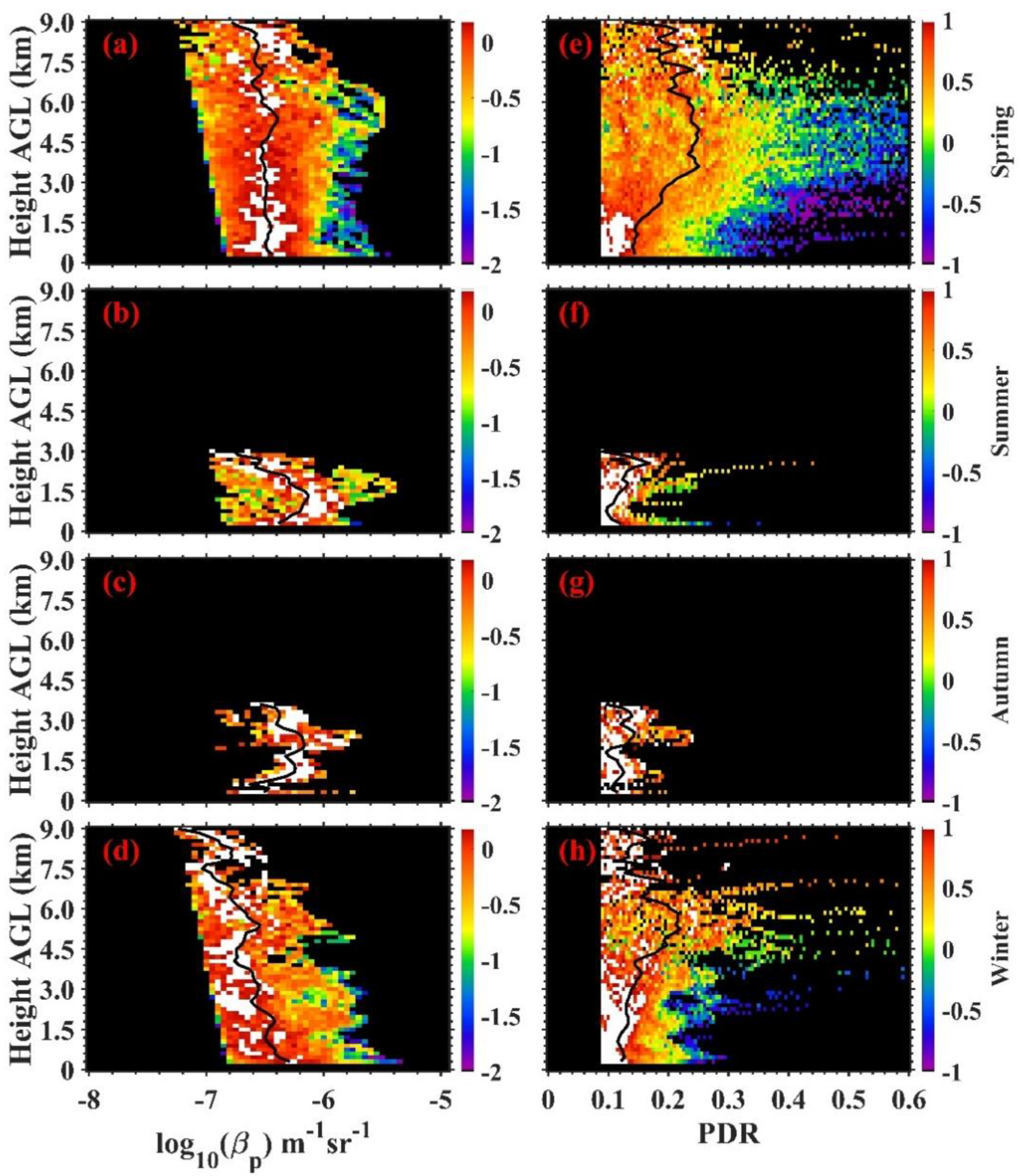
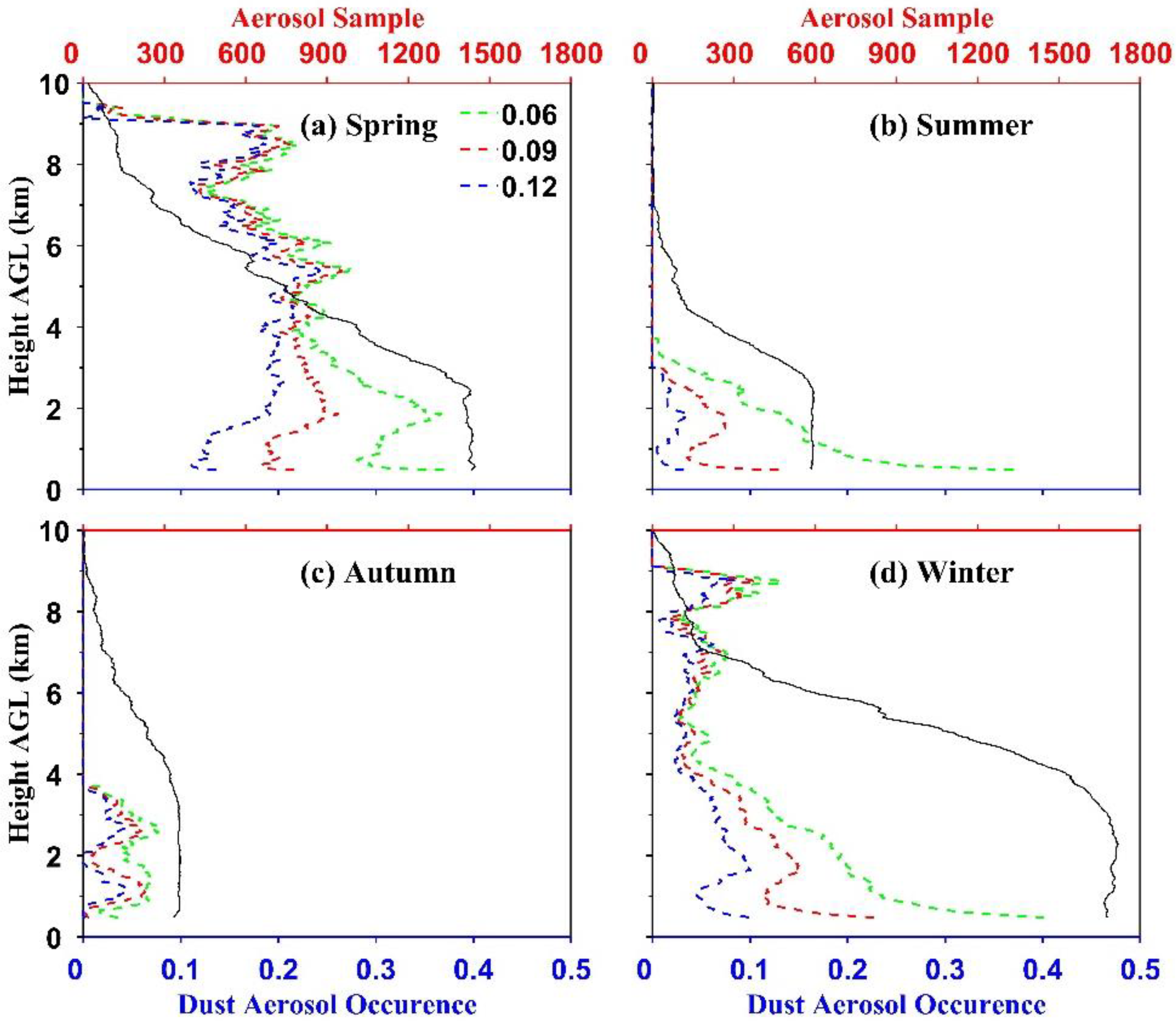
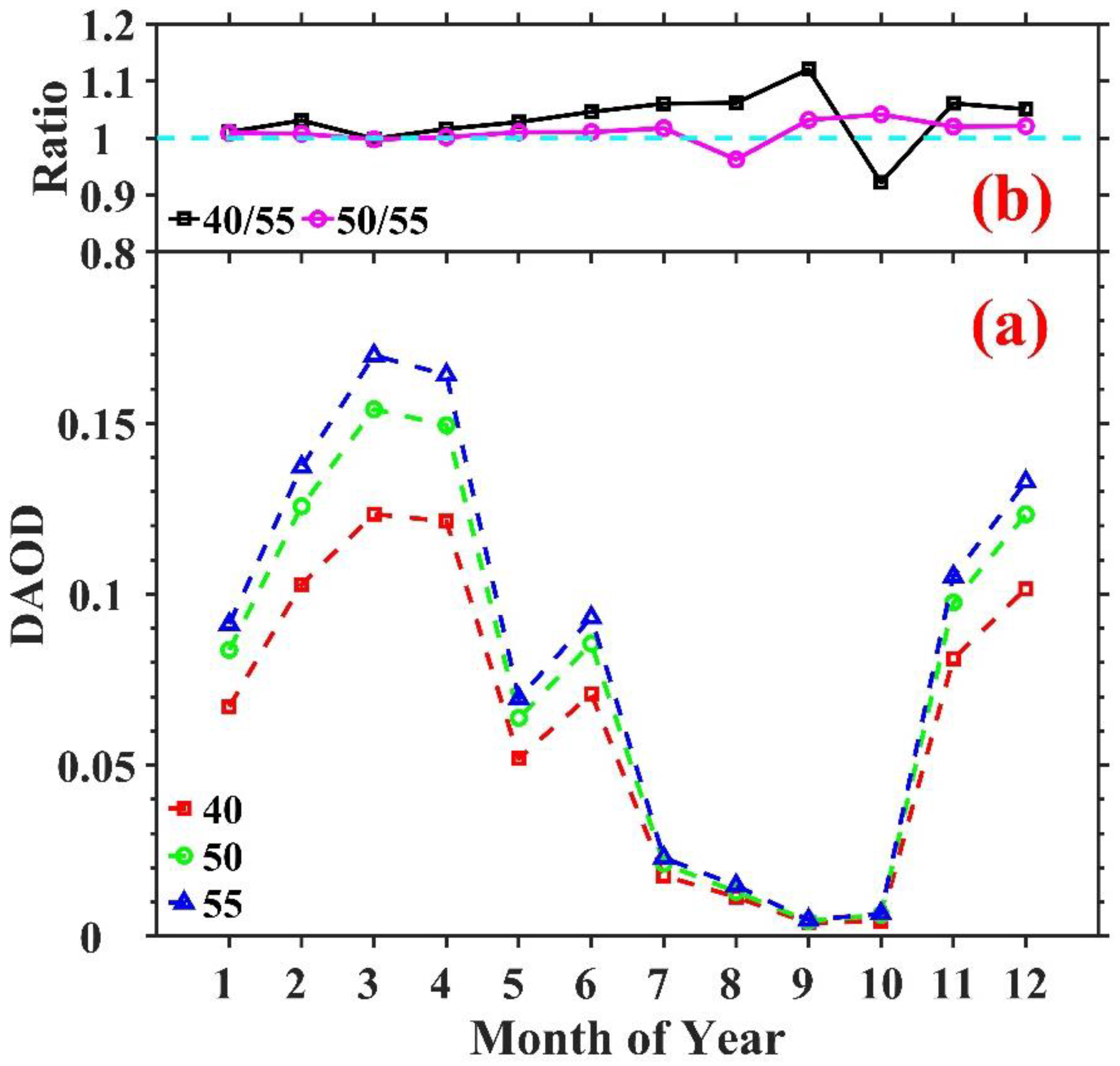
3.2. Seasonal Variations of Dust Aerosols

Figure 4 shows the seasonal cycle of MPL-derived dust aerosol backscatter coefficient and PDR profiles from January 2013 to September 2017 at the NSA site. This analysis is bases on cloud-free profiles. Dust aerosol is an important component of the Arctic haze. Dust aerosols occur in winter and spring in the entire troposphere, and in summer and autumn in the low (0–2 km) and middle (2–5 km) troposphere. These results are consistent with the seasonality of Arctic haze [29,37]. In the upper troposphere (5–10 km) dust aerosols occurring during the late winter and early spring (January–April) are likely associated with the long-range transportation of natural and anthropogenic aerosols from low-latitude areas including Eurasia, Siberia, North America, and Southeast Asia [6,7,25,26]. Further, Yang et al. [44] showed that polar jets can carry dust aerosols from source regions to the Arctic with CALIOP measurement. There are few low-dust aerosol occurrences and small aerosol samples (red line of Figure 4c) during August–October. A high occurrence of thin and opaque clouds during summer and autumn is responsible for the low samples during this period [36,85]. Long-range dust transportation from middle latitudes is weak [44], but wet deposition is obvious in this period [86]. Thus, dust aerosols during August–October are primarily from local and regional emissions [42].

Figure 5 shows the vertical distributions (every 150 m) of seasonal particulate backscatter coefficient (Figure 5a–d) and PDR PDFs (Figure 5e–h) based on MPL measurements at the NSA site from January 2013 to September 2017. The corresponding seasonal averaged profiles (black lines) of backscatter coefficient and PDR are over-plotted, separately. In summer and autumn, the backscatter coefficients of dust aerosols are relatively large, but PDR is small, implying that they may be the local dusty marine aerosols [87]. In winter and spring, dust aerosols are detected in the entire troposphere. The mean profiles of aerosol backscatter coefficients and PDRs of dust aerosols show that the strongest are in middle and upper troposphere in spring. The vertical PDF distribution in spring is broader than in winter. This indicates that spring dust aerosols have the more complex mixture states of dust and non-dust aerosols due to the long-range transportation from the mid-latitudes [37,41,78,88,89,90,91].

Figure 6 shows the seasonal aerosol samples and dust occurrences. The number of the aerosol samples (black line in Figure 6) decreases with height for all seasons. The maximum amount of aerosol samples is in winter, and the minimum amount of aerosol samples is in autumn due to the seasonal cycle of clouds in the Arctic [7]. For the dust aerosol occurrences using PDR threshold 0.09 (red line in Figure 6), the maximum occurs in spring and the minimum occurs in autumn [92]. The maximum of occurrence profiles indicate that Arctic dust aerosols occur in three dust aerosol layers: 0–4 km, 4–8 km and 8–10 km during spring and winter, which is consistent with the example given in Figure 2. The dust aerosol occurrence is less than 0.1 in autumn and summer.

To quantify the uncertainty of the selected threshold on dust aerosol occurrences, the results within 30% of selected thresholds (0.09 $\pm$ 0.09 * 30%) (green, red, and blue lines in Figure 6) were compared. The PDR values can be interpreted as the different ratios of pure dust in all aerosols [93], which means that higher PDR values reflect the more dust aerosols mixed. For example, the dust occurrences with 0.06 are higher, especially below 4 km, which infers that there are more non-dust aerosols included. Below 4 km, the difference between dust aerosol occurrences with 0.12 and 0.09 are much smaller than the difference between 0.06 and 0.09. Above 4 km, dust occurrences have small difference among the three thresholds, which implies that dust aerosols are the dominant aerosol types in the Arctic upper troposphere. To balance between including as many dust aerosols as possible and avoiding non-dust aerosols, a PDR threshold of 0.09 was selected.

To derive the dust aerosol optical depth (DAOD), the dust aerosol extinction profile is needed, which is calculated by the multiplication of the retrieved particulate backscatter coefficients and assumed lidar ratio. The DAOD is the vertical integration of extinction profiles in the entire height range. For the seasonal variation of DAOD (Figure 7), the maximum is in later winter and early spring and the minimum is in late summer and early autumn, which is consistent with the trend and values of DAOD in the previous studies [94,95].

Here, the different lidar ratios are used to show the effect of lidar ratios on monthly DAOD retrievals. Figure 7a shows that the seasonality of DAODs with different lidar ratios is almost consistent except for the absolute values. To prove the small effect of lidar ratio on the monthly DAOD retrievals, the ratio of DAOD with different lidar ratios (black and magenta lines in Figure 7b) is calculated. The ratio is almost 5% except for the values in July–October (5–10%), which may result from small samples during these months.

4. Conclusions

A four-year and nine-month altitude-resolved distribution of MPL retrieved backscatter coefficient and PDR of Arctic dust aerosols at NSA site from January 2013 to September 2017 is presented. The long-term and stable MPL retrieved results and the comparison of MPL and co-located HSRL are shown for the first time, indicating the high quality of MPL retrievals. The dust aerosols are identified with PDR. The seasonality of Arctic dust aerosols shows the maximum is in late winter and early spring extending in the entire troposphere, which is from the long-range transportation of the mid-latitude dust aerosols, and the minimum is in the early summer and late autumn occurring in the low and middle troposphere, which originates from the local and regional sources.

Our understanding of the processes that control the Arctic aerosol properties remains highly uncertain. Research efforts are needed to constrain the seasonality and vertical profiles of Arctic aerosols to improve the model skills in simulation [7,22,96,97] and the ability of understanding aerosol-cloud-climate impacts [26]. The high occurrence of dust aerosols in Arctic highlighted the importance to simulate dust aerosols and their impacts on mixed-phase and ice clouds reliably. Our multi-year temporal distribution of MPL backscatter coefficient and PDR over the Arctic will provide a new dataset to validate these processes in global models. The limitation of ground-based MPL measurements is just one-point observations. In the future, the satellite such as CALIOP and SAGE can be combined to provide more information for the Arctic dust aerosol distributions.

References

1. Landrum, L.; Holland, M.M. Extremes become routine in an emerging new Arctic. Nat Clim Chang. 2020, 10, 1108–1156. [Google Scholar] [CrossRef]
2. Mauritsen, T.; Sedlar, J.; Tjernstrom, M.; Leck, C.; Martin, M.; Shupe, M.; Sjogren, S.; Sierau, B.; Persson, P.O.G.; Brooks, I.M.; et al. An Arctic CCN-limited cloud-aerosol regime. Atmos. Chem. Phys. 2011, 11, 165–173. [Google Scholar] [CrossRef] [Green Version]
3. Pithan, F.; Svensson, G.; Caballero, R.; Chechin, D.; Cronin, T.W.; Ekman, A.M.L.; Neggers, R.; Shupe, M.D.; Solomon, A.; Tjernstrom, M.; et al. Role of air-mass transformations in exchange between the Arctic and mid-latitudes. Nat. Geosci. 2018, 11, 805–812. [Google Scholar] [CrossRef]
4. Regayre, L.A.; Pringle, K.J.; Booth, B.B.B.; Lee, L.A.; Mann, G.W.; Browse, J.; Woodhouse, M.T.; Rap, A.; Reddington, C.L.; Carslaw, K.S. Uncertainty in the magnitude of aerosol-cloud radiative forcing over recent decades. Geophys. Res. Lett. 2014, 41, 9040–9049. [Google Scholar] [CrossRef]
5. DeMott, P.J.; Prenni, A.J.; Liu, X.; Kreidenweis, S.M.; Petters, M.D.; Twohy, C.H.; Richardson, M.S.; Eidhammer, T.; Rogers, D.C. Predicting global atmospheric ice nuclei distributions and their impacts on climate. Proc. Natl. Acad. Sci. USA 2010, 107, 11217–11222. [Google Scholar] [CrossRef] [Green Version]
6. Schmale, J.; Zieger, P.; Ekman, A.M.L. Aerosols in current and future Arctic climate. Nat Clim Chang. 2021, 11, 95–105. [Google Scholar] [CrossRef]
7. Willis, M.D.; Leaitch, W.R.; Abbatt, J.P.D. Processes Controlling the Composition and Abundance of Arctic Aerosol. Rev. Geophys. 2018, 56, 621–671. [Google Scholar] [CrossRef] [Green Version]
8. Shi, Y.; Liu, X.; Wu, M.; Zhao, X.; Ke, Z.; Brown, H. Relative importance of high-latitude local and long-range-transported dust for Arctic ice-nucleating particles and impacts on Arctic mixed-phase clouds. Atmos. Chem. Phys. 2022, 22, 2909–2935. [Google Scholar] [CrossRef]
9. Tobo, Y.; Adachi, K.; DeMott, P.J.; Hill, T.C.J.; Hamilton, D.S.; Mahowald, N.M.; Nagatsuka, N.; Ohata, S.; Uetake, J.; Kondo, Y.; et al. Glacially sourced dust as a potentially significant source of ice nucleating particles. Nat. Geosci. 2019, 12, 253–258. [Google Scholar] [CrossRef]
10. Karydis, V.A.; Kumar, P.; Barahona, D.; Sokolik, I.N.; Nenes, A. On the effect of dust particles on global cloud condensation nuclei and cloud droplet number. J. Geophys. Res.-Atmos. 2011, 116, D23. [Google Scholar] [CrossRef]
11. Korolev, A.; McFarquhar, G.; Field, P.R.; Franklin, C.; Lawson, P.; Wang, Z.; Williams, E.; Abel, S.J.; Axisa, D.; Borrmann, S. Mixed-phase clouds: Progress and challenges. Meteorol. Monogr. 2017, 58, 5.1–5.50. [Google Scholar] [CrossRef]
12. Zhang, D.M.; Wang, Z.; Heymsfield, A.; Fan, J.W.; Liu, D.; Zhao, M. Quantifying the impact of dust on heterogeneous ice generation in midlevel supercooled stratiform clouds. Geophys. Res. Lett. 2012, 39. [Google Scholar] [CrossRef] [Green Version]
13. Curry, J.A. Interactions among Turbulence, Radiation and Microphysics in Arctic Stratus Clouds. J. Atmos. Sci. 1986, 43, 90–106. [Google Scholar] [CrossRef]
14. Shupe, M.D.; Turner, D.D.; Zwink, A.; Thieman, M.M.; Mlawer, E.J.; Shippert, T. Deriving Arctic Cloud Microphysics at Barrow, Alaska: Algorithms, Results, and Radiative Closure. J. Appl. Meteorol. Clim. 2015, 54, 1675–1689. [Google Scholar] [CrossRef]
15. Zhang, D.; Wang, Z.; Luo, T.; Yin, Y.; Flynn, C. The occurrence of ice production in slightly supercooled Arctic stratiform clouds as observed by ground-based remote sensors at the ARM NSA site. J. Geophys. Res. Atmos. 2017, 122, 2867–2877. [Google Scholar] [CrossRef]
16. Zhao, M.; Wang, Z.E. Comparison of Arctic clouds between European Center for Medium-Range Weather Forecasts simulations and Atmospheric Radiation Measurement Climate Research Facility long-term observations at the North Slope of Alaska Barrow site. J. Geophys. Res.-Atmos. 2010, 115, adeed. [Google Scholar] [CrossRef]
17. Silber, I.; Fridlind, A.M.; Verlinde, J.; Russell, L.M.; Ackerman, A.S. Nonturbulent Liquid-Bearing Polar Clouds: Observed Frequency of Occurrence and Simulated Sensitivity to Gravity Waves. Geophys. Res. Lett. 2020, 47, e2020GL087099. [Google Scholar] [CrossRef]
18. Tan, I.; Storelvmo, T. Evidence of Strong Contributions From Mixed-Phase Clouds to Arctic Climate Change. Geophys. Res. Lett. 2019, 46, 2894–2902. [Google Scholar] [CrossRef] [Green Version]
19. Zelinka, M.D.; Myers, T.A.; Mccoy, D.T.; Po-Chedley, S.; Caldwell, P.M.; Ceppi, P.; Klein, S.A.; Taylor, K.E. Causes of Higher Climate Sensitivity in CMIP6 Models. Geophys. Res. Lett. 2020, 47, e2019GL085782. [Google Scholar] [CrossRef] [Green Version]
20. Mishra, A.K.; Koren, I.; Rudich, Y. Effect of aerosol vertical distribution on aerosol-radiation interaction: A theoretical prospect. Heliyon 2015, 1, e00036. [Google Scholar] [CrossRef]
21. Ukhov, A.; Mostamandi, S.; da Silva, A.; Flemming, J.; Alshehri, Y.; Shevchenko, I.; Stenchikov, G. Assessment of natural and anthropogenic aerosol air pollution in the Middle East using MERRA-2, CAMS data assimilation products, and high-resolution WRF-Chem model simulations. Atmos. Chem. Phys. 2020, 20, 9281–9310. [Google Scholar] [CrossRef]
22. Koffi, B.; Schulz, M.; Breon, F.-M.; Dentener, F.; Steensen, B.M.; Griesfeller, J.; Winker, D.; Balkanski, Y.; Bauer, S.E.; Bellouin, N.; et al. Evaluation of the aerosol vertical distribution in global aerosol models through comparison against CALIOP measurements: AeroCom phase II results. J. Geophys. Res-Atmos. 2016, 121, 7254–7283. [Google Scholar] [CrossRef] [PubMed] [Green Version]
23. Huneeus, N.; Schulz, M.; Balkanski, Y.; Griesfeller, J.; Prospero, J.; Kinne, S.; Bauer, S.; Boucher, O.; Chin, M.; Dentener, F.; et al. Global dust model intercomparison in AeroCom phase I. Atmos. Chem. Phys. 2011, 11, 7781–7816. [Google Scholar] [CrossRef] [Green Version]
24. Schmeisser, L.; Backman, J.; Ogren, J.A.; Andrews, E.; Asmi, E.; Starkweather, S.; Uttal, T.; Fiebig, M.; Sharma, S.; Eleftheriadis, K.; et al. Seasonality of aerosol optical properties in the Arctic. Atmos. Chem. Phys. 2018, 18, 11599–11622. [Google Scholar] [CrossRef] [Green Version]
25. Garrett, T.; Zhao, C.; Novelli, P. Assessing the relative contributions of transport efficiency and scavenging to seasonal variability in Arctic aerosol. Tellus B Chem. Phys. Meteorol. 2010, 62, 190–196. [Google Scholar] [CrossRef]
26. Arnold, S.R.; Law, K.S.; Brock, C.A.; Thomas, J.L.; Starkweather, S.M.; von Salzen, K.; Stohl, A.; Sharma, S.; Lund, M.T.; Flanner, M.G.; et al. Arctic air pollution: Challenges and opportunities for the next decade. Elementa-Sci. Anthr. 2016, 4, 104. [Google Scholar] [CrossRef] [Green Version]
27. Tomasi, C.; Kokhanovsky, A.A.; Lupi, A.; Ritter, C.; Smirnov, A.; O’Neill, N.T.; Stone, R.S.; Holben, B.N.; Nyeki, S.; Wehrli, C.; et al. Aerosol remote sensing in polar regions. Earth-Sci. Rev. 2015, 140, 108–157. [Google Scholar] [CrossRef] [Green Version]
28. Mitchell, J.M. Visual range in the polar regions with particular reference to the Alaskan Arctic. J. Atmos. Terr. Phys 1957, 17, 195–211. [Google Scholar]
29. Quinn, P.K.; Shaw, G.; Andrews, E.; Dutton, E.G.; Ruoho-Airola, T.; Gong, S.L. Arctic haze: Current trends and knowledge gaps. Tellus Ser. B-Chem. Phys. Meteorol. 2007, 59, 99–114. [Google Scholar] [CrossRef] [Green Version]
30. Ancellet, G.; Pelon, J.; Blanchard, Y.; Quennehen, B.; Bazureau, A.; Law, K.S.; Schwarzenboeck, A. Transport of aerosol to the Arctic: Analysis of CALIOP and French aircraft data during the spring 2008 POLARCAT campaign. Atmos. Chem. Phys. 2014, 14, 8235–8254. [Google Scholar] [CrossRef] [Green Version]
31. de Villiers, R.A.; Ancellet, G.; Pelon, J.; Quennehen, B.; Schwarzenboeck, A.; Gayet, J.F.; Law, K.S. Airborne measurements of aerosol optical properties related to early spring transport of mid-latitude sources into the Arctic. Atmos. Chem. Phys. 2010, 10, 5011–5030. [Google Scholar] [CrossRef]
32. Nott, G.J.; Duck, T.J. Lidar studies of the polar troposphere. Meteorol. Appl. 2011, 18, 383–405. [Google Scholar] [CrossRef]
33. Ritter, C.; Neuber, R.; Schulz, A.; Markowicz, K.; Stachlewska, I.; Lisok, J.; Makuch, P.; Pakszys, P.; Markuszewski, P.; Rozwadowska, A. 2014 iAREA campaign on aerosol in Spitsbergen–Part 2: Optical properties from Raman-lidar and in-situ observations at Ny-Ålesund. Atmos. Environ. 2016, 141, 1–19. [Google Scholar] [CrossRef] [Green Version]
34. Di Biagio, C.; Pelon, J.; Ancellet, G.; Bazureau, A.; Mariage, V. Sources, Load, Vertical Distribution, and Fate of Wintertime Aerosols North of Svalbard From Combined V4 CALIOP Data, Ground-Based IAOOS Lidar Observations and Trajectory Analysis. J. Geophys. Res.-Atmos. 2018, 123, 1363–1383. [Google Scholar] [CrossRef]
35. Devasthale, A.; Tjernström, M.; Omar, A.H. The vertical distribution of thin features over the Arctic analysed from CALIPSO observations. Tellus B Chem. Phys. Meteorol. 2011, 63, 86–95. [Google Scholar] [CrossRef] [Green Version]
36. Treffeisen, R.E.; Thomason, L.W.; Strom, J.; Herber, A.B.; Burton, S.P.; Yamanouchi, T. Stratospheric Aerosol and Gas Experiment (SAGE) II and III aerosol extinction measurements in the Arctic middle and upper troposphere. J. Geophys. Res.-Atmos. 2006, 111, D17203. [Google Scholar] [CrossRef] [Green Version]
37. Di Pierro, M.; Jaeglé, L.; Eloranta, E.W.; Sharma, S. Spatial and seasonal distribution of Arctic aerosols observed by the CALIOP satellite instrument (2006–2012). Atmos. Chem. Phys. 2013, 13, 7075–7095. [Google Scholar] [CrossRef] [Green Version]
38. Yang, Y.K.; Zhao, C.F.; Wang, Q.; Cong, Z.Y.; Yang, X.C.; Fan, H. Aerosol characteristics at the three poles of the Earth as characterized by Cloud-Aerosol Lidar and Infrared Pathfinder Satellite Observations. Atmos. Chem. Phys. 2021, 21, 4849–4868. [Google Scholar] [CrossRef]
39. Shibata, T.; Shiraishi, K.; Shiobara, M.; Iwasaki, S.; Takano, T. Seasonal Variations in High Arctic Free Tropospheric Aerosols Over Ny-Alesund, Svalbard, Observed by Ground-Based Lidar. J. Geophys. Res.-Atmos. 2018, 123, 12353–12367. [Google Scholar] [CrossRef]
40. Zhang, D.; Comstock, J.; Xie, H.; Wang, Z. Polar Aerosol Vertical Structures and Characteristics Observed with a High Spectral Resolution Lidar at the ARM NSA Observatory. Remote Sens. 2022, 14, 4638. [Google Scholar] [CrossRef]
41. Pernov, J.B.; Beddows, D.; Thomas, D.C.; Dall’Osto, M.; Harrison, R.M.; Schmale, J.; Skov, H.; Massling, A. Increased aerosol concentrations in the High Arctic attributable to changing atmospheric transport patterns. Npj Clim. Atmos. Sci. 2022, 5, 62. [Google Scholar] [CrossRef]
42. Schmale, J.; Sharma, S.; Decesari, S.; Pernov, J.; Massling, A.; Hansson, H.C.; von Salzen, K.; Skov, H.; Andrews, E.; Quinn, P.K.; et al. Pan-Arctic seasonal cycles and long-term trends of aerosol properties from 10 observatories. Atmos. Chem. Phys. 2022, 22, 3067–3096. [Google Scholar] [CrossRef]
43. Bullard, J.E.; Baddock, M.; Bradwell, T.; Crusius, J.; Darlington, E.; Gaiero, D.; Gassó, S.; Gisladottir, G.; Hodgkins, R.; McCulloch, R.; et al. High-latitude dust in the Earth system. Rev. Geophys. 2016, 54, 447–485. [Google Scholar] [CrossRef] [Green Version]
44. Yang, K.; Wang, Z.E.; Luo, T.; Liu, X.H.; Wu, M.X. Upper troposphere dust belt formation processes vary seasonally and spatially in the Northern Hemisphere. Commun. Earth Environ. 2022, 3, 24. [Google Scholar] [CrossRef]
45. Zwaaftink, C.D.; Grythe, H.; Skov, H.; Stohl, A. Substantial contribution of northern high-latitude sources to mineral dust in the Arctic. J. Geophys. Res. Atmos. 2016, 121, 13678–13697. [Google Scholar] [CrossRef] [PubMed]
46. Dagsson-Waldhauserova, P.; Renard, J.B.; Olafsson, H.; Vignelles, D.; Berthet, G.; Verdier, N.; Duverger, V. Vertical distribution of aerosols in dust storms during the Arctic winter. Sci. Rep. 2019, 9, 16122. [Google Scholar] [CrossRef] [Green Version]
47. Xie, H.L.; Wang, Z.E.; Zhou, T.; Yang, K.; Liu, X.H.; Fu, Q.; Zhang, D.M.; Deng, M. Afterpulse correction for micro-pulse lidar to improve middle and upper tropospheric aerosol measurements. Opt. Express 2021, 29, 43502–43515. [Google Scholar] [CrossRef]
48. Verlinde, J.; Zak, B.; Shupe, M.; Ivey, M.; Stamnes, K. The arm north slope of alaska (nsa) sites. Meteorol. Monogr. 2016, 57, 8.1–8.13. [Google Scholar] [CrossRef]
49. Flynn, C.J.; Mendozaa, A.; Zhengb, Y.; Mathurb, S. Novel polarization-sensitive micropulse lidar mearsurement technique. Opt. Express 2007, 15, 2785–2790. [Google Scholar] [CrossRef]
50. Muradyan, P.; Coulter, R. Micropulse Lidar (MPL) Handbook; PNNL: Richland, WA, USA, 2020. [Google Scholar]
51. Campbell, J.R.; Hlavka, D.L.; Welton, E.J.; Flynn, C.J.; Turner, D.D.; Spinhirne, J.D.; Scott, V.S.; Hwang, I.H. Full-time, eye-safe cloud and aerosol lidar observation at atmospheric radiation measurement program sites: Instruments and data processing. J. Atmos. Ocean. Technol. 2002, 19, 431–442. [Google Scholar] [CrossRef]
52. Goldsmith, J. High Spectral Resolution Lidar (HSRL) Instrument Handbook; ARM Climate Research Facility, Pacific Northwest National Laboratory: Richland, WA, USA, 2016. [Google Scholar]
53. Eloranta, E.E. High spectral resolution lidar. In Lidar; Springer: Berlin/Heidelberg, Germany, 2005; pp. 143–163. [Google Scholar]
54. Kacenelenbogen, M.; Vaughan, M.A.; Redemann, J.; Hoff, R.M.; Rogers, R.R.; Ferrare, R.A.; Russell, P.B.; Hostetler, C.A.; Hair, J.W.; Holben, B.N. An accuracy assessment of the CALIOP/CALIPSO version 2/version 3 daytime aerosol extinction product based on a detailed multi-sensor, multi-platform case study. Atmos. Chem. Phys. 2011, 11, 3981–4000. [Google Scholar] [CrossRef]
55. Kollias, P.; Clothiaux, E.E.; Ackerman, T.P.; Albrecht, B.A.; Widener, K.B.; Moran, K.P.; Luke, E.P.; Johnson, K.L.; Bharadwaj, N.; Mead, J.B.; et al. Development and applications of ARM millimeter-wavelength cloud radars. Meteorol. Monogr. 2016, 57, 17.11–17.19. [Google Scholar] [CrossRef]
56. Bucholtz, A. Rayleigh-Scattering Calculations for the Terrestrial Atmosphere. Appl. Optics. 1995, 34, 2765–2773. [Google Scholar] [CrossRef] [PubMed]
57. Xie, H.; Zhou, T.; Fu, Q.; Huang, J.; Huang, Z.; Bi, J.; Shi, J.; Zhang, B.; Ge, J. Automated detection of cloud and aerosol features with SACOL micro-pulse lidar in northwest China. Opt. Express 2017, 25, 30732–30753. [Google Scholar] [CrossRef]
58. Fernald, F.G. Analysis of Atmospheric Lidar Observations—Some Comments. Appl. Optics. 1984, 23, 652–653. [Google Scholar] [CrossRef]
59. Omar, A.H.; Winker, D.M.; Kittaka, C.; Vaughan, M.A.; Liu, Z.Y.; Hu, Y.X.; Trepte, C.R.; Rogers, R.R.; Ferrare, R.A.; Lee, K.P.; et al. The CALIPSO Automated Aerosol Classification and Lidar Ratio Selection Algorithm. J. Atmos. Ocean. Technol. 2009, 26, 1994–2014. [Google Scholar] [CrossRef]
60. Liu, Z.; Liu, D.; Huang, J.; Vaughan, M.; Uno, I.; Sugimoto, N.; Kittaka, C.; Trepte, C.; Wang, Z.; Hostetler, C.; et al. Airborne dust distributions over the Tibetan Plateau and surrounding areas derived from the first year of CALIPSO lidar observations. Atmos. Chem. Phys. 2008, 8, 5045–5060. [Google Scholar] [CrossRef] [Green Version]
61. Baars, H.; Kanitz, T.; Engelmann, R.; Althausen, D.; Heese, B.; Komppula, M.; Preissler, J.; Tesche, M.; Ansmann, A.; Wandinger, U.; et al. An overview of the first decade of Polly(NET): An emerging network of automated Raman-polarization lidars for continuous aerosol profiling. Atmos. Chem. Phys. 2016, 16, 5111–5137. [Google Scholar] [CrossRef] [Green Version]
62. Freudenthaler, V. Lidar Rayleigh-fit criteria. In Proceedings of the EARLINET-ASOS 7th Workshop, Madrid, Spain, 9–11 February 2009. [Google Scholar]
63. Freudenthaler, V.; Esselborn, M.; Wiegner, M.; Heese, B.; Tesche, M.; Ansmann, A.; Muller, D.; Althausen, D.; Wirth, M.; Fix, A.; et al. Depolarization ratio profiling at several wavelengths in pure Saharan dust during SAMUM 2006. Tellus Ser. B-Chem. Phys. Meteorol. 2009, 61, 165–179. [Google Scholar] [CrossRef] [Green Version]
64. Behrendt, A.; Nakamura, T. Calculation of the calibration constant of polarization lidar and its dependency on atmospheric temperature. Opt. Express 2002, 10, 805–817. [Google Scholar] [CrossRef]
65. Burton, S.P.; Hair, J.W.; Kahnert, M.; Ferrare, R.A.; Hostetler, C.A.; Cook, A.L.; Harper, D.B.; Berkoff, T.A.; Seaman, S.T.; Collins, J.E.; et al. Observations of the spectral dependence of linear particle depolarization ratio of aerosols using NASA Langley airborne High Spectral Resolution Lidar. Atmos. Chem. Phys. 2015, 15, 13453–13473. [Google Scholar] [CrossRef]
66. Cairo, F.; Di Donfrancesco, G.; Adriani, A.; Pulvirenti, L.; Fierli, F. Comparison of various linear depolarization parameters measured by lidar. Appl. Optics. 1999, 38, 4425–4432. [Google Scholar] [CrossRef] [PubMed]
67. Burton, S.P.; Ferrare, R.A.; Hostetler, C.A.; Hair, J.W.; Rogers, R.R.; Obland, M.D.; Butler, C.F.; Cook, A.L.; Harper, D.B.; Froyd, K.D. Aerosol classification using airborne High Spectral Resolution Lidar measurements—Methodology and examples. Atmos. Meas. Technol. 2012, 5, 73–98. [Google Scholar] [CrossRef] [Green Version]
68. Sassen, K. The polarization lidar technique for cloud research: A review and current assessment. B. Am. Meteorol. Soc. 1991, 72, 1848–1866. [Google Scholar] [CrossRef]
69. Liu, D.; Wang, Z.; Liu, Z.; Winker, D.; Trepte, C. A height resolved global view of dust aerosols from the first year CALIPSO lidar measurements. J. Geophys. Res. Atmos. 2008, 113, D16214. [Google Scholar] [CrossRef]
70. Luo, T.; Wang, Z.; Zhang, D.; Liu, X.; Wang, Y.; Yuan, R. Global dust distribution from improved thin dust layer detection using A-train satellite lidar observations. Geophys. Res. Lett. 2015, 42, 620–628. [Google Scholar] [CrossRef]
71. Zhou, T.; Xie, H.L.; Bi, J.R.; Huang, Z.W.; Huang, J.P.; Shi, J.S.; Zhang, B.D.; Zhang, W. Lidar Measurements of Dust Aerosols during Three Field Campaigns in 2010, 2011 and 2012 over Northwestern China. Atmosphere 2018, 9, 173. [Google Scholar] [CrossRef] [Green Version]
72. Groß, S.; Esselborn, M.; Weinzierl, B.; Wirth, M.; Fix, A.; Petzold, A. Aerosol classification by airborne high spectral resolution lidar observations. Atmos. Chem. Phys. 2013, 13, 2487–2505. [Google Scholar] [CrossRef] [Green Version]
73. Groß, S.; Tesche, M.; Freudenthaler, V.; Toledano, C.; Wiegner, M.; Ansmann, A.; Althausen, D.; Seefeldner, M. Characterization of Saharan dust, marine aerosols and mixtures of biomass-burning aerosols and dust by means of multi-wavelength depolarization and Raman lidar measurements during SAMUM 2. Tellus B Chem. Phys. Meteorol. 2011, 63, 706–724. [Google Scholar] [CrossRef]
74. Illingworth, A.J.; Barker, H.W.; Beljaars, A.; Ceccaldi, M.; Chepfer, H.; Clerbaux, N.; Cole, J.; Delanoe, J.; Domenech, C.; Donovan, D.P.; et al. THE EARTHCARE SATELLITE The Next Step Forward in Global Measurements of Clouds, Aerosols, Precipitation, and Radiation. B. Am. Meteorol. Soc. 2015, 96, 1311–1332. [Google Scholar] [CrossRef] [Green Version]
75. Xie, C.; Nishizawa, T.; Sugimoto, N.; Matsui, I.; Wang, Z. Characteristics of aerosol optical properties in pollution and Asian dust episodes over Beijing, China. Appl. Opt. 2008, 47, 4945–4951. [Google Scholar] [CrossRef]
76. Baars, H.; Ansmann, A.; Althausen, D.; Engelmann, R.; Heese, B.; Muller, D.; Artaxo, P.; Paixao, M.; Pauliquevis, T.; Souza, R. Aerosol profiling with lidar in the Amazon Basin during the wet and dry season. J. Geophys. Res.-Atmos. 2012, 117, D21201. [Google Scholar] [CrossRef]
77. Bohlmann, S.; Baars, H.; Radenz, M.; Engelmann, R.; Macke, A. Ship-borne aerosol profiling with lidar over the Atlantic Ocean: From pure marine conditions to complex dust-smoke mixtures. Atmos. Chem. Phys. 2018, 18, 9661–9679. [Google Scholar] [CrossRef] [Green Version]
78. Stohl, A. Characteristics of atmospheric transport into the Arctic troposphere. J. Geophys. Res.-Atmos. 2006, 111, D11306. [Google Scholar] [CrossRef]
79. Liu, D.; Wang, Y.; Wang, Z.; Zhou, J. The three-dimensional structure of transatlantic African dust transport: A new perspective from CALIPSO LIDAR measurements. Adv. Meteorol. 2012, 2012, 1–9. [Google Scholar] [CrossRef] [Green Version]
80. Amiridis, V.; Wandinger, U.; Marinou, E.; Giannakaki, E.; Tsekeri, A.; Basart, S.; Kazadzis, S.; Gkikas, A.; Taylor, M.; Baldasano, J.; et al. Optimizing CALIPSO Saharan dust retrievals. Atmos. Chem. Phys. 2013, 13, 12089–12106. [Google Scholar] [CrossRef] [Green Version]
81. Painemal, D.; Clayton, M.; Ferrare, R.; Burton, S.; Josset, D.; Vaughan, M. Novel aerosol extinction coefficients and lidar ratios over the ocean from CALIPSO-CloudSat: Evaluation and global statistics. Atmos. Meas. Tech. 2019, 12, 2201–2217. [Google Scholar] [CrossRef] [Green Version]
82. Winker, D.M.; Tackett, J.L.; Getzewich, B.J.; Liu, Z.; Vaughan, M.A.; Rogers, R.R. The global 3-D distribution of tropospheric aerosols as characterized by CALIOP. Atmos. Chem. Phys. 2013, 13, 3345–3361. [Google Scholar] [CrossRef] [Green Version]
83. Gao, X.; Cao, X.; Wang, J.; Guo, Q.; Du, T.; Zhang, L. Analysis of aerosol optical properties in a Lanzhou suburb of China. Atmos. Res. 2020, 246, 105098. [Google Scholar] [CrossRef]
84. Kafle, D.N.; Coulter, R.L. Micropulse lidar-derived aerosol optical depth climatology at ARM sites worldwide. J. Geophys. Res-Atmos. 2013, 118, 7293–7308. [Google Scholar] [CrossRef]
85. Dong, X.Q.; Xi, B.K.; Crosby, K.; Long, C.N.; Stone, R.S.; Shupe, M.D. A 10 year climatology of Arctic cloud fraction and radiative forcing at Barrow, Alaska. J. Geophys. Res.-Atmos. 2010, 115, D17212. [Google Scholar] [CrossRef]
86. Mahmood, R.; von Salzen, K.; Flanner, M.; Sand, M.; Langner, J.; Wang, H.L.; Huang, L. Seasonality of global and Arctic black carbon processes in the Arctic Monitoring and Assessment Programme models. J. Geophys. Res.-Atmos. 2016, 121, 7100–7116. [Google Scholar] [CrossRef] [PubMed] [Green Version]
87. Song, C.B.; Dall’Osto, M.; Lupi, A.; Mazzola, M.; Traversi, R.; Becagli, S.; Gilardoni, S.; Vratolis, S.; Yttri, K.E.; Beddows, D.C.S.; et al. Differentiation of coarse-mode anthropogenic, marine and dust particles in the High Arctic islands of Svalbard. Atmos. Chem. Phys. 2021, 21, 11317–11335. [Google Scholar] [CrossRef]
88. Francis, D.; Eayrs, C.; Chaboureau, J.P.; Mote, T.; Holland, D.M. Polar Jet Associated Circulation Triggered a Saharan Cyclone and Derived the Poleward Transport of the African Dust Generated by the Cyclone. J. Geophys. Res.-Atmos. 2018, 123, 11899–11917. [Google Scholar] [CrossRef]
89. Varga, G.; Dagsson-Waldhauserova, P.; Gresina, F.; Helgadottir, A. Saharan dust and giant quartz particle transport towards Iceland. Sci. Rep. 2021, 11, 1–12. [Google Scholar] [CrossRef]
90. Zhao, X.; Huang, K.; Fu, J.S.; Abdullaev, S.F. Long-range transport of Asian dust to the Arctic: Identification of transport pathways, evolution of aerosol optical properties, and impact assessment on surface albedo changes. Atmos. Chem. Phys. 2022, 22, 10389–10407. [Google Scholar] [CrossRef]
91. Zwaaftink, C.D.G.; Arnalds, O.; Dagsson-Waldhauserova, P.; Eckhardt, S.; Prospero, J.M.; Stohl, A. Temporal and spatial variability of Icelandic dust emissions and atmospheric transport. Atmos. Chem. Phys. 2017, 17, 10865–10878. [Google Scholar] [CrossRef] [Green Version]
92. Fan, S.M. Modeling of observed mineral dust aerosols in the arctic and the impact on winter season low-level clouds. J. Geophys. Res.-Atmos. 2013, 118, 11161–11174. [Google Scholar] [CrossRef]
93. Luo, T.; Wang, Z.E.; Ferrare, R.A.; Hostetler, C.A.; Yuan, R.M.; Zhang, D.M. Vertically resolved separation of dust and other aerosol types by a new lidar depolarization method. Opt. Express 2015, 23, 14095–14107. [Google Scholar] [CrossRef]
94. Breider, T.J.; Mickley, L.J.; Jacob, D.J.; Wang, Q.Q.; Fisher, J.A.; Chang, R.Y.W.; Alexander, B. Annual distributions and sources of Arctic aerosol components, aerosol optical depth, and aerosol absorption. J. Geophys. Res.-Atmos. 2014, 119, 4107–4124. [Google Scholar] [CrossRef]
95. Yin, B.S.; Min, Q.L. Climatology of aerosol and cloud optical properties at the Atmospheric Radiation Measurements Climate Research Facility Barrow and Atqasuk sites. J. Geophys. Res.-Atmos. 2014, 119, 1820–1834. [Google Scholar] [CrossRef]
96. Wu, C.L.; Lin, Z.H.; Liu, X.H. The global dust cycle and uncertainty in CMIP5 (Coupled Model Intercomparison Project phase 5) models. Atmos. Chem. Phys. 2020, 20, 10401–10425. [Google Scholar] [CrossRef]
97. Wu, M.X.; Liu, X.H.; Yu, H.B.; Wang, H.L.; Shi, Y.; Yang, K.; Darmenov, A.; Wu, C.L.; Wang, Z.E.; Luo, T.; et al. Understanding processes that control dust spatial distributions with global climate models and satellite observations. Atmos. Chem. Phys. 2020, 20, 13835–13855. [Google Scholar] [CrossRef]
Figure 1. The probability density functions (PDF) of particle depolarization ratio (PDR) for all aerosols observed by MPL from January 2013 to September 2017 at the NSA site. The black line is for all the aerosols derived from MPL observations, while the red and green lines indicate non-dust and dust aerosol modes fitted to the shape of the PDF of all aerosol PDR. A PDR of 0.10 is the cross point of the dust and non-dust aerosol modes.
Remotesensing 14 05581 g001
Figure 2. The time-height section of (a) HSRL particular backscatter coefficients, (b) MPL retrieved particular backscatter coefficients, (c) MPL total volume depolarization ratio (VDR), and (d) MPL particle depolarization ratio (PDR) from February 11 to 14, 2015 at the NSA site. (ad) are for all aerosols. (e) MPL backscatter coefficient for dust aerosols that are identified using the PDR threshold 0.09.
Remotesensing 14 05581 g002
Figure 3. (a) The comparison of MPL (blue box) and HSRL (magenta box) backscatter coefficient vertical quartile distributions at the NSA site from January 2013 to September 2017. Box and whisker plots include the median, 25th and 75th percentiles (left and right of the boxes), and 5th and 95th percentiles (left and right of the whiskers). The red and cyan lines are for the medians of HSRL and MPL, respectively. (b) The ratio of MPL and HSRL backscatter medians.
Remotesensing 14 05581 g003
Figure 4. The climatological month–altitude sections of dust aerosols (a) particular backscatter coefficients and (b) PDR, and (c) aerosol samples (red line) and dust occurrence (blue line) for cloud-free profiles from MPL at the NSA site from January 2013 to September 2017. The dust occurrence is defined as the ratio of dust aerosol samples and all aerosol samples. The samples are based on the data with 1 h and 30 m bin.
Remotesensing 14 05581 g004
Figure 5. The vertical PDF distribution of seasonal particulate backscatter coefficients (ad) and PDR for MPL (eh) at the NSA site from January 2013 to September 2017. Rows from top to bottom are for spring (a,e), summer (b,f), autumn (c,g) and winter (d,h), separately. The seasonal average profiles (black lines) are plotted in each sub-figure. The color bar is the log scale of PDF distribution values of particular backscatter coefficients and PDR in each 150 m.
Remotesensing 14 05581 g005
Figure 6. The aerosol samples (black line) in (a) spring, (b) summer, (c) autumn and (d) winter, and dust aerosol occurrences using the PDR thresholds of 0.06 (green line), 0.09 (red line) and 0.12 (blue line) for MPL measurements at the NSA site from January 2013 to September 2017. The samples are based on the data with 1 h and 30 m bin.
Remotesensing 14 05581 g006
Figure 7. The seasonal cycle of (a) dust aerosol optical depth (DAOD) with lidar ratios of 40 sr (red line), 50 sr (green line) and 55 sr (blue line) for MPL measurements at the NSA site from January 2013 to September 2017. (b) The ratio of DAODs with different lidar ratios (cyan line is the reference line, black line is the ratio of 40 and 55, magenta line is the ratio of 50 and 55).
Remotesensing 14 05581 g007
Publisher’s Note: MDPI stays neutral with regard to jurisdictional claims in published maps and institutional affiliations.