Multi-Sensor Fusion Based Estimation of Tire-Road Peak Adhesion Coefficient Considering Model Uncertainty

Abstract

The tire-road peak adhesion coefficient (TRPAC), which cannot be directly measured by on-board sensors, is essential to road traffic safety. Reliable TRPAC estimation can not only serve the vehicle active safety system, but also benefit the safety of other traffic participants. In this paper, a TRPAC fusion estimation method considering model uncertainty is proposed. Based on virtual sensing theory, an image-based fusion estimator considering the uncertainty of the deep-learning model and the kinematic model is designed to realize the accurate classification of the road surface condition on which the vehicle will travel in the future. Then, a dynamics-image-based fusion estimator considering the uncertainty of visual information is proposed based on gain scheduling theory. The results of simulation and real vehicle experiments show that the proposed fusion estimation method can make full use of multisource sensor information, and has significant advantages in estimation accuracy, convergence speed and estimation robustness compared with other single-source-based estimators.

1. Introduction

1.1. Motivation

The interaction force between the tire and the road is the result of the complex interaction between the tire rubber and the road surface, and the interaction force is also one of the main factors affecting the stability of the vehicle chassis [1,2]. The tire-road peak adhesion coefficient (TRPAC) is defined as the ratio of the tire peak adhesion force to the tire vertical load, which can characterize the tire-road adhesion ability. If precise and real-time TRPAC estimation of the current road can be realized, it is possible to minimize the probability of serious traffic accidents under harsh road surface conditions (e.g., slippery roads, snow-covered roads, etc.). TRPAC is one of the important factors to ensure the safety of traffic participants. However, TRPAC cannot be directly measured by on-board sensors.

1.2. Related Work

TRPAC is especially critical for automotive active safety control systems, such as anti-lock braking system (ABS) and traction control system (TCS). Many scholars have proposed TRPAC estimation methods based on the tire dynamic response measured by low-cost on-board sensors. The tire dynamics-based methods can be mainly divided into two categories: longitudinal dynamics-based and lateral dynamics-based methods. Longitudinal dynamics-based estimation methods mainly depend on the relationship between the longitudinal tire force and slip rate in the tire model. Generally, state observers based on different tire models (e.g., Magic Formula [3], Burckhardt [4], LuGre [5]) were designed to estimate TRPAC under acceleration and braking conditions. Lateral dynamics-based estimation methods are mainly established based on the relationship between the lateral tire force or tire alignment torque and the tire slip angle in the tire model. Based on Brush [6,7], TMSimple [8,9] and other tire models, Kalman filter-based or state observer-based methods were extensively studied to estimate TRPAC under steering maneuver conditions.

The working conditions of dynamics-based estimators (DEs) are easily satisfied based on the vehicle state data provided by on-board sensors. However, the identification accuracy of DEs strongly depends on the tire modeling accuracy. In addition, sufficient road excitation is necessary to ensure the obvious differences in the tire mechanical characteristic curves under different road adhesion conditions. In highly dynamic and complex excitation conditions, the convergence speed and accuracy of DE will face severe challenges.

With the improvement of vehicle intelligence, an increasing number of vehicles are equipped with environmental perception sensors, such as cameras and lidars. The perception information fed back by such sensors is predictive, which brings a new development opportunity for research on vehicle state parameter estimation [10]. Considering that cameras are the primary sensors for intelligent vehicles, the representative literature on image-based estimators (IEs) will be reviewed below. The image texture and color feature information extracted by the gray level co-occurrence matrix was utilized to train a support vector machine (SVM) for the classification of road surface conditions [11,12,13]. In recent years, convolutional neural networks have been widely employed in various fields. Roychowdhury et al. [14] designed a deep learning-based two-stage estimation method to classify roads into snow, slush, wet and dry asphalt. Cheng et al. [15] proposed a deep learning-based method for the classification of road surface condition, and a new activation function was constructed to make the model have better generalization and classification performance. Based on high-definition cameras, Du et al. [16] used a local binarization algorithm and gray-level co-occurrence matrix to extract the spatial feature texture information of road images and concatenated the feature information into a modified VGGNet to estimate road adhesion levels. Since the camera can sense the driving road ahead in advance, the estimation results of IEs are predictive and there is no need for specific road excitation input. However, the disadvantage is that it is easily disturbed by external environmental factors, which will cause the degradation of sensor measurement information and aggravate the uncertainty of the model [17].

Considering the advantages of different sensors, some scholars designed fusion estimation methods based on multi-sensor fusion. Considering the noise of the sensor, Chen et al. [18] proposed a fusion estimation method based on data fusion in the frequency domain, which used the frequency spectrum of the in-wheel motor drive system and the steering system to obtain the longitudinal and lateral dynamic responses, respectively. Then the recursive least square algorithm was applied to estimate TRPAC. Combining the predictability of IE and the robustness of DE, Svensson et al. [19] proposed a fusion estimation method based on Gaussian process regression. However, the tuning of hyperparameters in Gaussian process regression limits the application of this method to different driving conditions. The overall performance of fusion estimation is bounded by the performance of a single estimator.

1.3. Contribution

In this paper, aided by prior visual information, a dynamics-image-based fusion estimator (DIFE) considering model uncertainty is proposed to accelerate the convergence rate of DE for accurate and robust TRPAC estimation. The main contributions of this paper are summarized as follows: (1) Considering the model uncertainty caused by external interference, an image-based fusion estimator (IFE) based on virtual sensing theory is proposed to output the identification results and visual information confidence of the upcoming road area ahead of the vehicle; (2) Combining the robustness of DE to external interference and the high sensitivity and predictability of IE for sudden changes in road surface conditions, a TRPAC fusion estimation method with the assessment of visual information confidence is established; (3) Simulation and real vehicle experiments were carried out for each module to verify the effectiveness of the proposed TRPAC fusion estimation method.

1.4. Paper Organization

The rest of this paper is organized as follows: In Section 2, a fusion estimation framework considering model uncertainty is constructed, which consists of an image-based fusion estimator (IFE) and a dynamics-image-based fusion estimator (DIFE). In Section 3, the IFE considering model uncertainty is described, including road feature identification module based on multi-task learning and temperature scaling, and a fusion identification module based on improved Dempster-Shafer evidence theory (DSET). The spatiotemporal transformation strategy for identification results is introduced. In Section 4, considering visual information confidence, a DIFE is established based on the fusion of DE and IFE. In Section 5, the performance validation of the proposed IFE is presented. Then, simulation and experimental validation are performed to test the effectiveness of the proposed DIFE. Finally, the conclusions are summarized in Section 6.

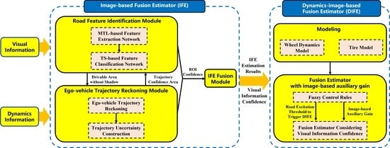
2. Estimation Framework

Considering the critical problems in the estimation of TRPAC, such as slow convergence and low accuracy caused by low-quality sensor information, a fusion estimation framework considering model uncertainty as shown in Figure 1 is designed, including an image-based fusion estimator, and a dynamics-image-based fusion estimator. The estimation process is as follows: (1) The road feature extraction network based on multi-task learning (MTL) is used to segment the drivable area without shadows; (2) The regions of interest are selected in the trajectory confidence ellipse region generated by the ego-vehicle trajectory reckoning module, considering the uncertainty of the kinematic model; (3) Considering the uncertainty of the deep learning model, the road feature classification network is calibrated with temperature scaling (TS) to output more reliable classification confidence of each region of interest; (4) Then, the IFE fusion module is used to fuse the confidence of each region of interest output by the calibrated road feature classification network; (5) Finally, a sequence of spatial distributions of IFE estimation results and visual information confidence is obtained as the prior information to make the proposed DIFE achieve reliable TRPAC estimation.

3. Design of Image-Based Fusion Estimator Considering Model Uncertainty

In order to extract the road surface features from the images collected by the front-view camera, IE based on the voting strategy [20] was proposed in our previous work. The main idea is to first use the semantic segmentation network to segment the drivable area and extract the regions of interest (ROIs) from the obtained drivable area segmentation mask. Based on the classification network model, the class with the largest number of votes will be determined as the identification result. Finally, the estimated TRPAC is obtained through the established mapping relationship between the classification result and the empirical value of TRPAC.

Since the light sensor of the camera is very sensitive to changes in the external environment, the image quality of the sensor will be greatly reduced under external interference such as road shadows, abnormal exposure, and motion blur. As a result, the performance of IE will also be greatly affected. Therefore, considering the common visual degradation factors mentioned above, an image-based fusion estimator is proposed to identify the road surface condition that the vehicle will travel in the future period.

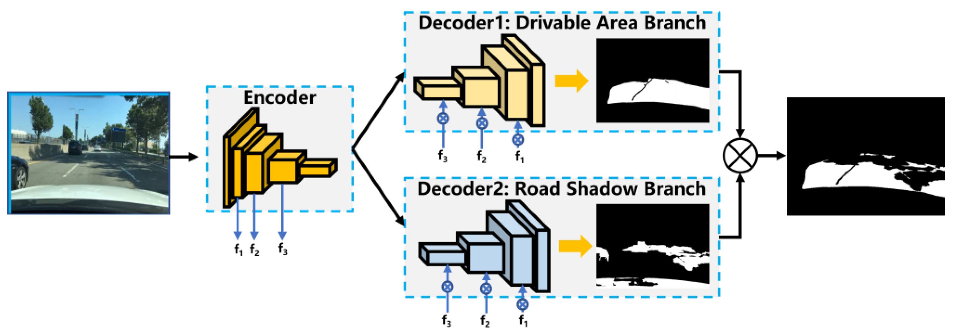
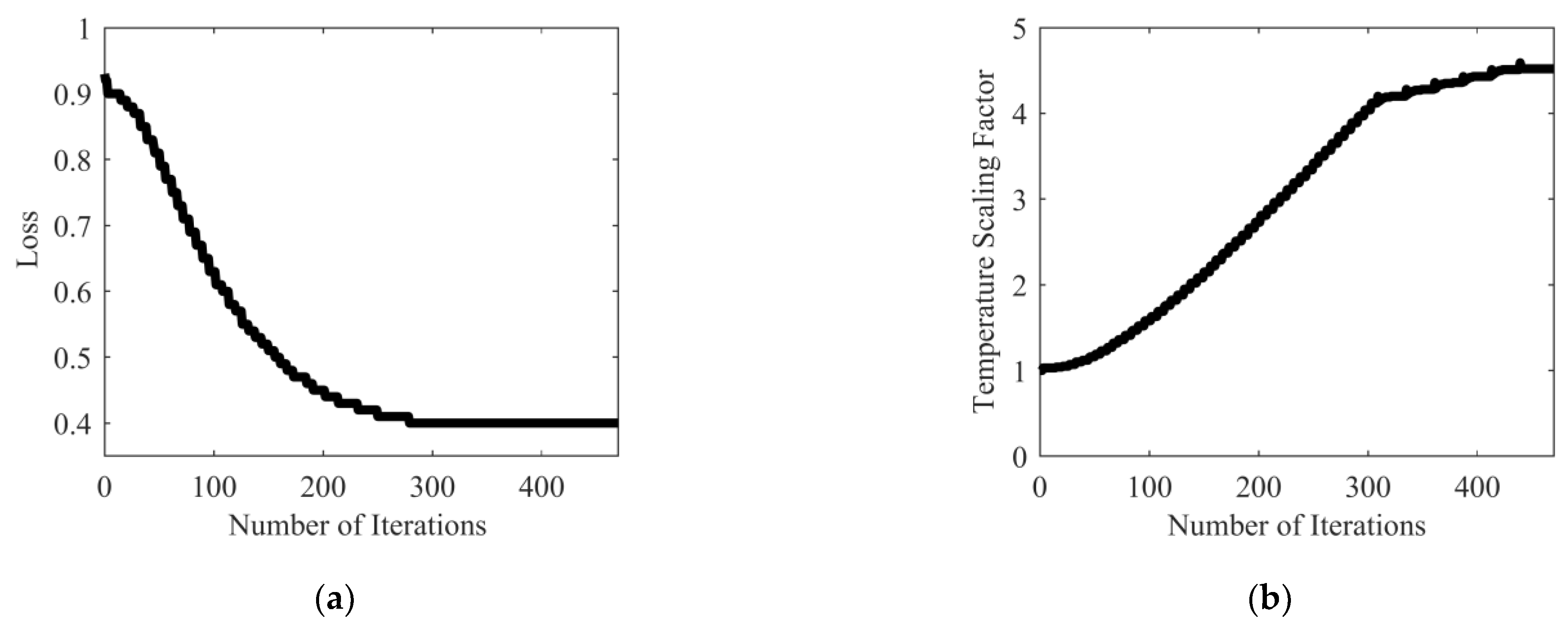
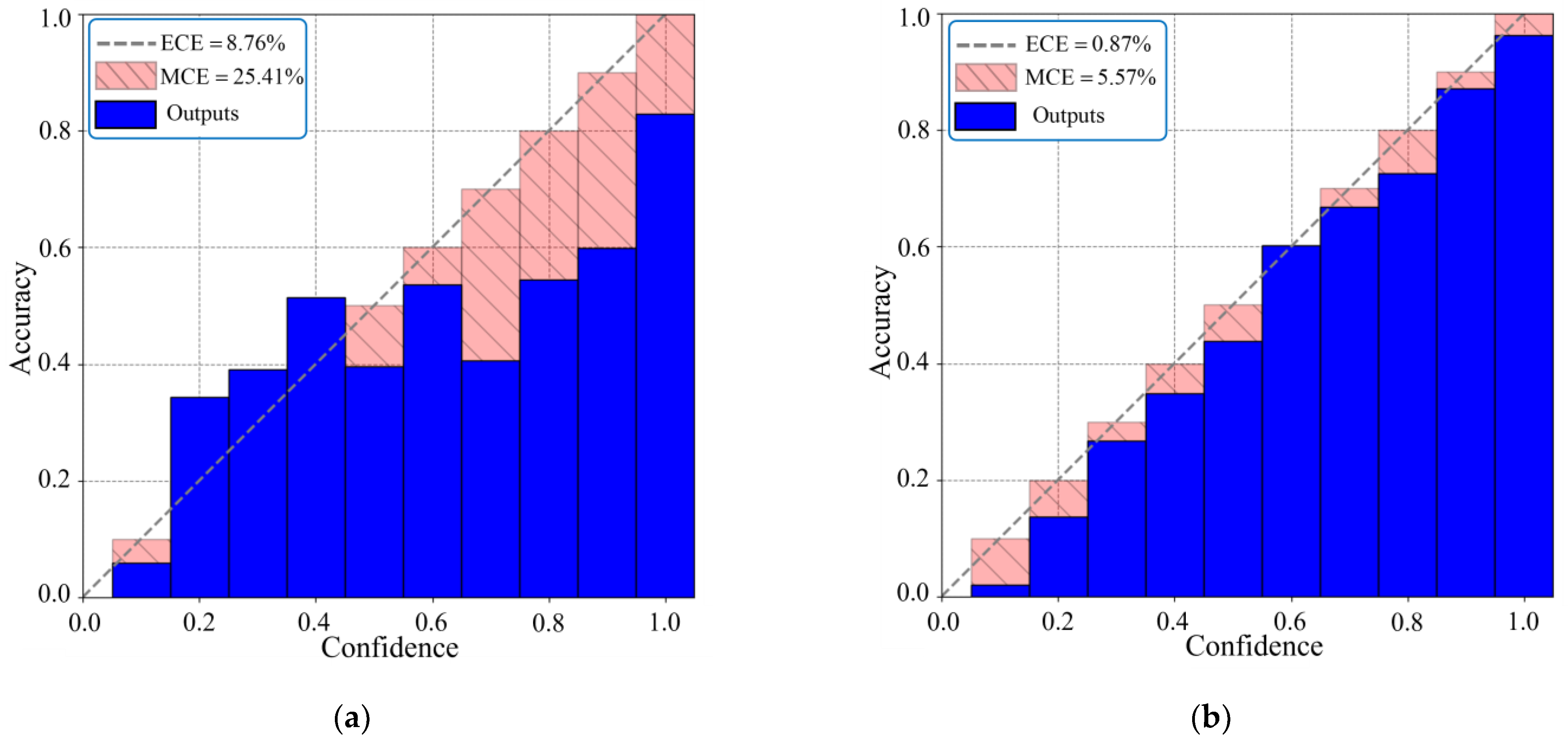
3.1. Road Feature Identification Module Considering Deep-Learning Model Uncertainty

As shown in Figure 2, the road feature extraction network is designed in our previous work [21]. The network structure is a typical encoder and decoder structure, and the network parameters of the encoder part are shared to the two decoder branches at the same time. Each decoder branch undertakes a segmentation task, namely, to achieve drivable area segmentation and road shadow segmentation.

Considering the computing power limitation of on-board equipment of intelligent vehicles, the lightweight neural network ShuffleNet [22] is selected as the road feature classification model. The basic unit of the ShuffleNet network is improved based on the residual module of ResNet. It mainly adopts point group convolution and channel random shuffling, which achieves the purpose of improving computational efficiency and maintaining classification accuracy. However, due to the inherent noise in the sample data and insufficient training samples, deep learning models suffer from aleatoric and epistemic uncertainty [23]. Therefore, the deep learning model still has limitations in high-risk application scenarios such as medical treatment and autonomous driving, and the uncertainty estimation of the model is of great significance in the above application fields.

For multi-classification tasks of road surface conditions, the uncertainty distribution of the model can be obtained by the confidence distribution output by the softmax layer of ShuffleNet. Due to the uncertainty of deep learning models, deep neural network models often suffer from overconfidence or underconfidence. The confidence of the model prediction results does not match the actual accuracy. The model calibration error can be evaluated based on the quantitative index: the expected calibration error (ECE) and the maximum calibration error (MCE) [24].

In order to train and calibrate the classification model, a structured road image dataset containing the samples disturbed by common visual degradation factors is constructed to expand the sample space of the validation set for subsequent model calibration. Figure 3 shows the samples of the road image dataset based on BDD100K and the self-collected road image dataset. The constructed road image dataset with noised samples contains common visual degradation factors (i.e., abnormal exposure, motion blur, road shadow). BDD100K provides image data of dry asphalt road and wet asphalt road. The self-collected dataset provides image data of snow/ice road and supplements the image data of dry asphalt road. The image data augmentation library Albumentations [25] is used to generate abnormal exposure and motion blur interference. Some abnormal exposure interference in the self-collected dataset is generated by adjusting the camera exposure gain.

Considering the large workload of manual extraction from the entire image, first the original road image data are divided according to the road surface condition (i.e., dry asphalt, wet asphalt and snow/ice). Then, the trained road feature extraction network model is used to automatically segment the drivable area and extract the road image parts. The distribution of the constructed road image part dataset is presented in

Table 1. The distribution of the constructed road image part dataset with noised samples.

Title 1	Dry Asphalt	Wet Asphalt	Snow/Ice
Training set (normal)	4258	2442	1214
Validation set (normal)	1075	617	299
Validation set (noised)	750	450	221

.

In Table 1, it is worth noting that the training set in the constructed dataset in this paper does not contain the road image parts extracted from the noised samples and only contains noised samples in the validation set. This can prevent the model from learning noised features to avoid a significant drop in the model’s prediction accuracy for regular samples. The training loss function is set to cross-entropy loss. The Adam optimizer is also used to train the model, and the initial learning rate is set to 0.0001.

Model calibration methods mainly include regularization calibration methods based on modified training loss function and postprocessing calibration methods based on validation set. Since the addition of noised samples in the training set will make the model learn relevant noised features, the regularization method based on adjusting the loss function may lead to the model underfitting, so the temperature scaling [24] in the postprocessing calibration method is chosen to calibrate the original ShuffleNet model.

Temperature scaling is a soft label smoothing technology. The main principle is to introduce a temperature coefficient $T$ into the original softmax function to smooth or sharpen the logic vector output by the model. When $T>1$, the information entropy of the confidence distribution of the model output will increase, and the model output will become smooth to alleviate the overconfidence of the model. When $T\in \left(0,1\right)$, the information entropy of the confidence distribution of the model output will decrease, and the model output will become sharp to alleviate the underconfidence of the model. In addition, since the temperature scaling factor $T$ is a parameter greater than zero, the order of the dimensions of the output logic vector after temperature scaling will not change. As a result, the model calibration method based on temperature scaling will not affect the classification performance of the model. The temperature scaling factor can be learned by optimizing the cross-entropy loss function of the validation set. The learning process of the temperature scaling factor is shown in Figure 3.

The reliability diagrams of the classification model before and after calibration are presented in Figure 4, respectively. As can be seen from Figure 4, the model confidence of the uncalibrated model does not match the actual average accuracy, and the degree of overconfidence is large. Overconfidence of the model is generally caused by the cross-entropy loss function used for training. During the training process of the model, only the dimension of the label corresponding to the maximum value in the confidence distribution participates in the calculation of the loss function, and the relationship between the real label and other labels is ignored, so the output of the model may be extremely biased toward one class, which makes the model overconfident. It can be seen from Figure 4b that both the expected calibration error (ECE) and the maximum calibration error (MCE) of the model are significantly reduced, indicating that the model is well calibrated.

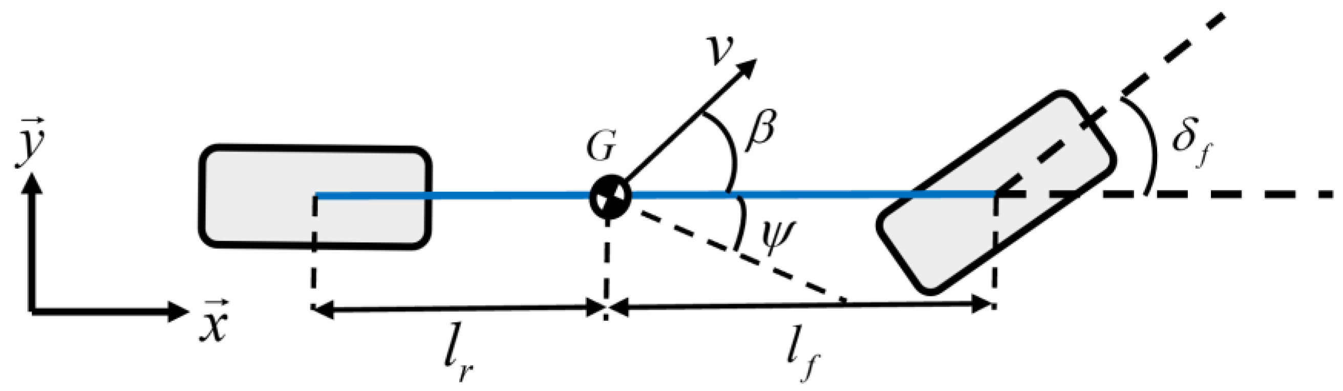
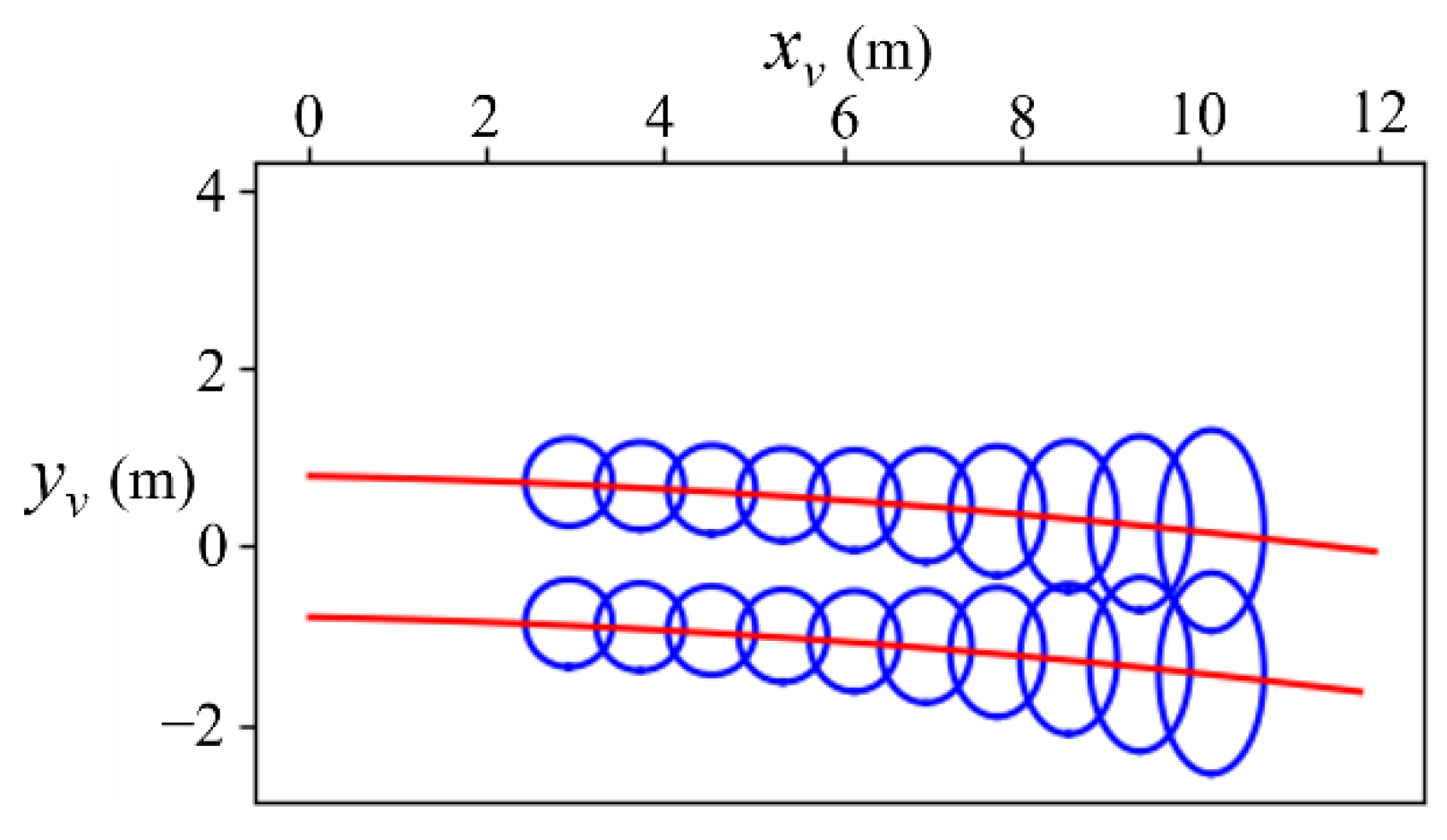
3.2. Ego-Vehicle Trajectory Reckoning Module Considering Kinematic Model Uncertainty

Existing image-based road recognition methods usually only process the front-view image provided by the camera. Due to the perspective effect of the obtained front-view image, the representative area of the obtained prediction result is often large, and the processing of irrelevant areas in the image may interfere with the final identification result and reduce the computational efficiency. Therefore, in order to accurately identify the road surface condition of the area that the front wheels will pass through, an ego-vehicle trajectory reckoning module considering kinematic model uncertainty is introduced.

Considering that most of the existing mass-produced vehicles are still at the partial driver assistance level below L3, there is no reference trajectory provided by the decision-making and planning system. In addition, most of the vehicle’s driving conditions do not involve extreme driving conditions, so the ego-vehicle trajectory is reckoned based on the extended kinematic bicycle model.

As shown in Figure 5, taking the vehicle acceleration $a$ and the front wheel steering angle ${\delta }_f$ as the control input, the vehicle single-track kinematics model in the inertial coordinate system can be established. In order to reckon the trajectory of the left and right front wheels, the single-track bicycle model can be extended to the double-track form, as shown in Equation (1).

$$\left\{\begin{array}{l}{x}_L(k)=x(k)+l_f\cos (\psi (k))-\frac{b}{2}\sin (\psi (k))\\ y_L(k)=y(k)+\frac{b}{2}\cos (\psi (k))+l_f\sin (\psi (k))\\ x_R(k)=x(k)+l_f\cos (\psi (k))+\frac{b}{2}\sin (\psi (k))\\ y_R(k)=y(k)-\frac{b}{2}\cos (\psi (k))+l_f\sin (\psi (k))\end{array}\right.$$

(1)

where $x_L$, $y_L$ are the horizontal and vertical coordinates of the left front wheel in the inertial coordinate system, respectively, $x_R$, $y_R$ are the horizontal and vertical coordinates of the right front wheel in the inertial coordinate system, respectively, and $b$ is the front wheel track, $\psi$ is the vehicle yaw angle, $v$ is the vehicle speed, and $l_f$, $l_r$ are the distances between the vehicle center of gravity and the front or rear axles, respectively.

Due to the uncertainty of driving behavior, the reckoned ego-vehicle trajectory based on the kinematic model will not be completely consistent with the real trajectory. Generally, it can be considered that the reckoned trajectory is relatively accurate in a short time, and the relative error of the reckoned trajectory in a long time is relatively large. Therefore, it is necessary to establish the uncertainty distribution to better characterize the trajectory distribution.

It can be seen from Equation (1) that the system variables that directly affect the reckoned trajectory are the coordinates of the vehicle center of gravity $x$, $y$ and the vehicle yaw angle $\psi$. For the modeling of vehicle state uncertainty, the uncertainty of the vehicle state can be described as a Gaussian distribution [26]. Therefore, the Gaussian distribution shown in Equation (2) is used to describe the uncertainty of the above system variables.

$${\displaystyle {\sum }_{x,y,\psi }\sim N\left(0,{\sigma }_{x,y,\psi }^2\right)}$$

(2)

Since the error of the reckoned trajectory will continue to be superimposed, assuming that the system state variable $X={\left[\begin{array}{cccc}x& y& v_x& v_y\end{array}\right]}^T$ changes linearly, the state prediction equation considering the uncertainty distribution is derived as follows.

$$\left\{\begin{array}{l}X\left(k+1\right)=FX\left(k\right)+W\\ P\left(k+1\right)=FP\left(k\right)F^T+Q\end{array}\right.$$

(3)

where $P$ represents the system uncertainty distribution (i.e., system covariance distribution), the definitions of the state transition matrix $F$ and the noise covariance matrix $Q$ are shown in Equation (4). Due to the high consistency of the lateral distribution of the road surface, in order to facilitate the extraction of ROIs, ${\sigma }_x^2=k_{1}v$ and ${\sigma }_y^2=k_{2}v$ ($k_1<k_2$) can be set.

$$F=\left[\begin{array}{cccc}1& 0& \Delta t& 0\\ 0& 1& 0& \Delta t\\ 0& 0& 1& 0\\ 0& 0& 0& 1\end{array}\right],\hspace{0.33em}Q=\left[\begin{array}{cccc}0& 0& 0& 0\\ 0& 0& 0& 0\\ 0& 0& {\sigma }_x^2& 0\\ 0& 0& 0& {\sigma }_y^2\end{array}\right]$$

(4)

where $\Delta t$ is the sampling period, ${\sigma }_x^2$ and ${\sigma }_y^2$ are the uncertainty variances of the horizontal and vertical coordinates of the vehicle center of gravity, respectively.

It can be seen from Equation (3) that with the increase of the recursion time, the uncertainty distribution variance of the reckoned trajectory will increase. Therefore, a 95% confidence ellipse with a certain step interval can be set to represent the uncertainty distribution of the reckoned trajectory.

3.3. Fusion Module Based on Improved DSET

In our previous work, the class corresponding to the maximum number of candidate ROIs in a frame is defined as the prediction result of the frame [20]. Considering that in real driving scenarios, the accuracy of model recognition cannot reach 100%. Moreover, it is easily interfered with by various external environmental factors, causing the estimation results to oscillate. Therefore, the image-based fusion module based on improved DSET is added for subsequent high-quality fusion of IE with DE. The main idea is to define candidate ROIs as virtual sensors to make them form redundant sensor networks. The confidence distribution output by the calibrated road feature classification model is defined as the evidence, and the visual information confidence of the candidate confidence ellipse region is defined. Then, the improved DSET is used to obtain the fusion prediction results and visual information confidence.

For the subsequent extraction of candidate ROIs, it is necessary to project the uncertainty distribution of the reckoned trajectory based on the vehicle coordinate system into the image coordinate system.

It is assumed that the road where the vehicle is located is flat, and the coordinate in the vehicle coordinate system is defined as $P_v={(x_v,\hspace{0.33em}{y}_v,\hspace{0.33em}0)}^T$. The origin of the vehicle coordinate system is the center of the front axle of the vehicle. The coordinate in the image coordinate system is $P_i={(x_i,\hspace{0.33em}{y}_i)}^T$, and the origin is the upper left corner pixel of the image. The coordinate in the camera coordinate system is $P_c={(x_c,\hspace{0.33em}{y}_c,\hspace{0.33em}{z}_c)}^T$. The following transformation relationship between the camera coordinate system and the image coordinate system is derived.

$$P_i=\frac{T_{ci}}{c_n}{P}_c$$

(5)

where $c_n$ is the normalization coefficient, and $T_{ci}$ is the camera internal parameter matrix obtained by calibration.

Based on Equation (5), the transformation relationship from the image coordinate system to the vehicle coordinate system can be expressed as:

$${\overline{P}}_i=\left(\frac{T_{ci}}{c_n}{T}_{cv}\right){\overline{P}}_v=H_{cv}\overline{P}$$

(6)

where ${\overline{P}}_v$ and ${\overline{P}}_i$ represent the normalized vehicle coordinate system coordinates and image coordinate system coordinates, respectively, $T_{cv}$ is the camera extrinsic parameter matrix obtained by calibration, and $H_{cv}$ is the transformation matrix from the vehicle coordinate system to the image coordinate system.

A sample of the reckoned trajectory and uncertainty distribution of the reckoned trajectory in the vehicle coordinate system is shown in Figure 6. The sample after projection to the image coordinate system is shown in Figure 7.

Considering that if the candidate ROIs are extracted directly based on the center of the candidate confidence ellipse within the reckoned trajectory, the following problems may be caused: (1) The extracted part of the road surface area is limited, and the identification result is easily disturbed by the external environment; (2) The identification results of the candidate ROI are not representative of the local region. In the image coordinate system, the feature details of the image near the vehicle are richer, and the feature details of the image far away from the vehicle are slightly blurred. Therefore, based on the distance from the vehicle, the confidence ellipses within the selected image regions can be grouped to extract candidate ROIs.

Based on the above analysis, a method for extracting candidate ROIs in the confidence ellipse region is proposed as shown in Figure 8. Firstly, the selected area in the vehicle coordinate system is divided into grids with size $a$, and then the coordinates of the corner points of the divided grids are projected and transformed. The total number of corner points covered by road shadows in the group of confidence ellipses $n_{rs}$, the total number of grid corner points in the group of confidence ellipses $n_{ell}$, and the proportion of non-shaded grid corner points in the group of confidence ellipses $p_{util}$ are calculated, respectively. If the number of remaining coverage grids in the confidence ellipse region without shadow coverage $\left(n_{ell}-n_{rs}\right)\le 1$, it means that the available area is too small, then exit the algorithm and continue to search for the next candidate group of confidence ellipses. Otherwise, the $b$ sets of grid corners are randomly sampled in the confidence ellipse region without shadow coverage according to the relative distance, and finally the sequence of candidate ROIs in the confidence ellipse region is output.

The extraction process of the proposed candidate ROIs extraction method is shown in Figure 9. It is worth noting that both the grid size $a$ and the random sampling group number of the grid corners $b$ will affect the extraction efficiency and accuracy of candidate ROIs. In this paper, $a=0.02 \mathrm{m}$ is selected based on reasonable experiments. Since the feature details in the confidence ellipse region with a farther distance from the vehicle are more blurred, it is necessary to sample the image features in the farther region multiple times and select $b= 4/6/8$, respectively.

After obtaining candidate ROIs, inspired by virtual sensing theory, a fusion method based on improved DSET is designed. A virtual sensor is a unique form of sensor, which outputs the required measurement information based on the established mathematical and statistical analysis model. The measurements derived from the mathematical model are defined as outputs of virtual sensors [27]. The candidate ROIs extracted in each frame are regarded as virtual sensors. The measurement information is defined as the predicted probability of each road surface condition output by the calibrated road feature classification model. Based on the rich measurement information of road surface conditions provided by the constructed redundant virtual sensor network, the improved DSET is used to fuse them to ensure the stability and accuracy of the IFE estimation results.

DSET is a data fusion method that can objectively deal with ambiguous and uncertain information. By combining the independent judgments of multiple incompatible bodies of evidence on the sub-propositions of the identification framework, more reliable conclusions can be drawn than with a single source of information [28].

In this paper, the DSET combinational rule can be derived as follows:

$$\left\{\begin{array}{l}K={\displaystyle \sum _{S_1\cap \cdots \cap S_n\ne \varnothing }\overline{m_1}(S_1)\cdot \overline{m_2}(S_2)\cdots \overline{m_n}(S_n)}\\ P_{Fusion}^{rd}=\frac{1}{K}{\displaystyle \sum _{S_1\cap S_2\cap \cdots \cap S_n=rd}\overline{m_1}(S_1)\cdot \overline{m_2}(S_2)\cdots \overline{m_n}(S_n),\hspace{0.33em}rd=dry,wet,snow}\end{array}\right.$$

(7)

where $S_n$ is defined as a virtual sensor (i.e., evidence in DSET), $\overline{m}(\cdot )$ is the basic probability assignment of each road surface condition in each piece of evidence, $K$ is the conflict coefficient, which can measure the degree of conflict between evidence, $P_{Fusion}^{rd}$ is the fusion confidence corresponding to a certain class of road surface condition.

However, the basic DSET still has the following two problems in practical applications: (1) The fusion problem when a strong conflict exists between evidence. The DSET combinational rule may not be able to combine the known evidence; (2) The problem of the basic probability assignment generation of evidence. The generation result of the basic probability assignment will directly affect the fusion result output by the system. The basic DSET defaults that the weight of each evidence is the same. When the evidence is strongly conflicting, it leads to abnormal fusion results.

In order to solve the problem of abnormal fusion results caused by strong conflicts between evidence, the historical identification results are used to assign different weights to the evidence corresponding to each road surface condition. As a result, a new basic probability assignment is constructed and the weights in it are updated online.

The constructed new basic probability assignment is shown in Equation (8).

$$\left\{\begin{array}{l}\overline{m}(rd)=\frac{w_{dry}\cdot {\displaystyle \sum P_{dry}}+w_{wet}\cdot {\displaystyle \sum P_{wet}}+w_{snow}\cdot {\displaystyle \sum P_{snow}}}{n_{dry}\cdot w_{dry}+n_{wet}\cdot w_{wet}+n_{snow}\cdot w_{snow}}\\ {\overline{m}}_0(rd)=\frac{\overline{m}(rd)}{\overline{m}(dry)+\overline{m}(wet)+\overline{m}(snow)},\hspace{0.33em}rd=dry,wet,snow\end{array}\right.$$

(8)

where $P_{dry}$, $P_{wet}$, and $P_{snow}$ represent the confidence of each class of candidate ROIs output by the road feature classification model, $w_{dry}$, $w_{wet}$, and $w_{snow}$ represent the evidence weight corresponding to different road surface conditions, $n_{dry}$, $n_{wet}$, and $n_{snow}$ represent the number of candidate ROIs classified as different road surface conditions, and ${\overline{m}}_0(rd)$ is the normalized basic probability assignment corresponding to a certain road surface condition.

Considering that the road surface condition changes very slowly within a certain sampling time, an online update strategy for the evidence weight shown in Equation (9) is proposed to make the fusion result as stable as possible. In addition, if there is no candidate ROI or only a single ROI in a certain frame, the class corresponding to the maximum weight value can be defined as the prediction result based on the historical information.

$$\left\{\begin{array}{l}{w}_{rd}^{-}\left(k\right)=\mathrm{sigmoid}\left[w_{rd}\left(k-1\right)+\sigma \cdot \left(\frac{n_{rd}}{n_{act}}-w_{rd}\left(k-1\right)\right)\right], rd=dry,wet,snow\\ w_{rd}\left(k\right)=\frac{w_{rd}^{-}\left(k\right)}{w_{dry}^{-}\left(k\right)+w_{wet}^{-}\left(k\right)+w_{snow}^{-}\left(k\right)}, rd=dry,wet,snow \end{array}\right.$$

(9)

where $w_{rd}^{-}\left(k\right)$ is the updated weight of the road surface condition $rd$ at time $k$, $w_{rd}\left(k-1\right)$ is the normalized weight of the road surface condition $rd$ at time $\left(k-1\right)$, $w_{rd}\left(k\right)$ is the normalized weight of road surface condition $rd$ at time $k$, $n_{act}$ is the total number of extracted candidate ROIs, $n_{rd}$ is the number of candidate ROIs predicted by ShuffleNet as road surface condition $rd$, and $\sigma$ is a relaxation factor that balances update rate and update stability.

Based on the candidate ROIs extraction method shown in Figure 8, the obtained sequence of candidate ROIs can be input into the calibrated road feature classification model for uncertainty distribution estimation. Based on the proposed fusion method based on improved DSET, the fusion prediction results and fusion confidence $P_i^{Fusion}$ in a single group of confidence ellipses can be obtained. Therefore, the visual information confidence $Q_v$ for a single group of confidence ellipses within the uncertainty distribution can be defined as follows.

$$Q_v=p_{util}\cdot P_i^{Fusion}$$

(10)

where $p_{util}$ is the proportion of the available area in the candidate confidence ellipse region of group $i$. Considering the subsequent fusion, the visual information confidence flag is defined. After a reasonable experiment, when $Q_v>0.5$, the flag is set to flag “1”.

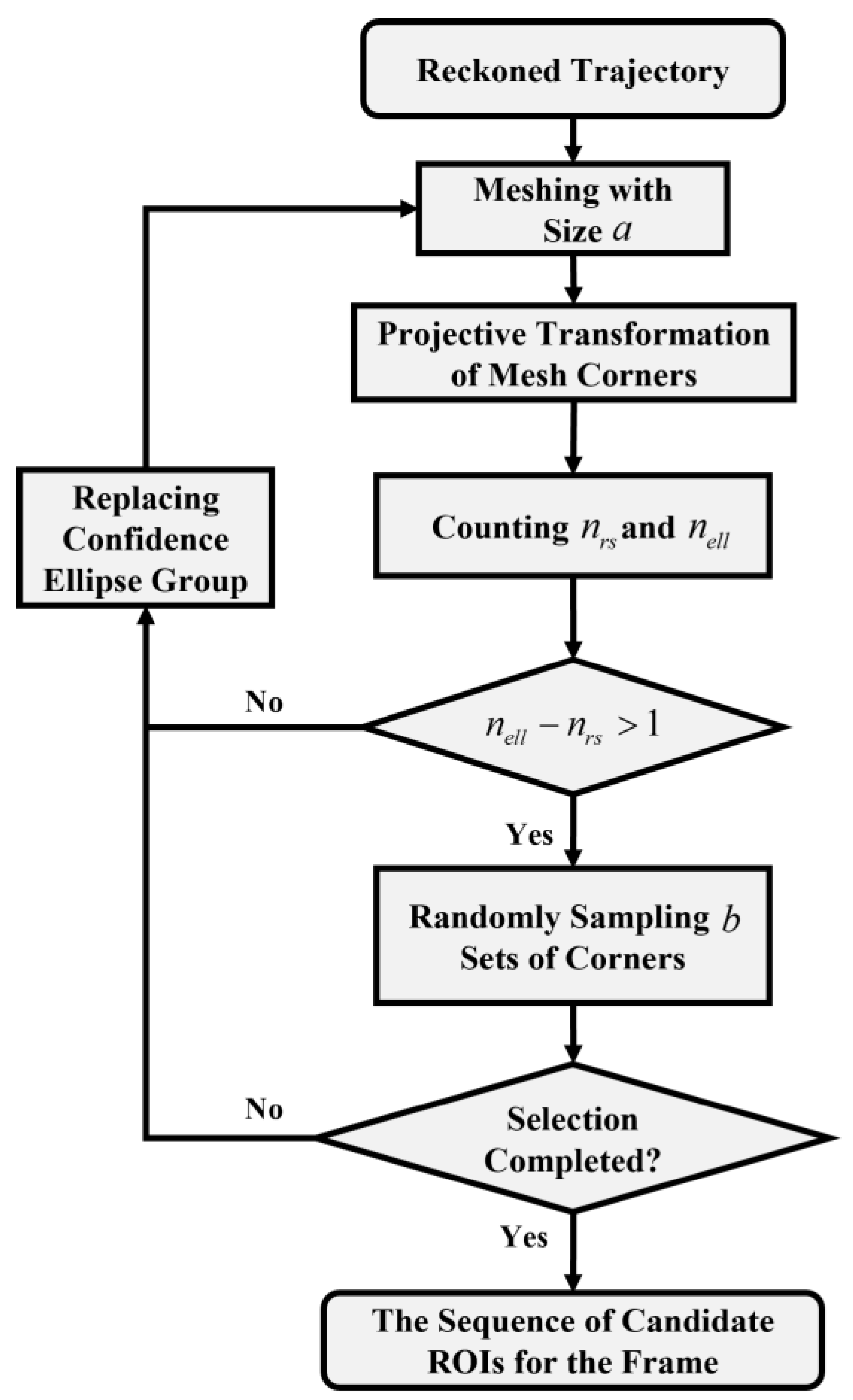
3.4. Spatiotemporal Transformation Strategy for Identification Results

Since the visual information is predictive, it is necessary to consider the algorithm processing time and the camera image acquisition cycle to perform spatiotemporal transformation processing on the identification results of the proposed IFE. The vehicle speed in the geodetic coordinate system is defined as $v_x$, and $P_0$ represents the preview distance from the image captured by the camera to the front wheel of the vehicle. When the algorithm finishes processing one frame, $P_2$ represents the current center position of the front wheel of the vehicle in the geodetic coordinate system derived from the reckoned trajectory. Considering that the feature details near the vehicle are rich, this paper chooses to update the identification results of each frame in real time, and then the displacement stamp $\left(X_{lb},X_{ub}\right)$ of the final identification results of the frame in the geodetic coordinate system can be obtained as follows.

$$\left\{\begin{array}{l}{X}_{lb}=P_2+P_0-{\displaystyle {\int }_0^{\Delta t_1}{v}_x }dt\\ X_{ub}=P_2+P_0-{\displaystyle {\int }_0^{\Delta t_1}{v}_x }dt+{\displaystyle {\int }_0^{\Delta t_2}{v}_x }dt\end{array}\right.$$

(11)

where $\Delta t_1$ is the processing time of the algorithm for one frame, and $\Delta t_2$ is the cycle time of the camera to capture the image. Here, $\Delta t_1=\Delta t_2$ is set for subsequent synchronization processing.

The spatial position relationship in the spatiotemporal transformation strategy is shown in Figure 10, including the image coordinate system and the vehicle coordinate system at the corresponding moment of the frame. $P_1$ is the vehicle’s front wheel position in the geodetic coordinate system when the camera captures the frame. After the algorithm processing time $\Delta t_2$, the vehicle reaches the position $P_2$ as shown in Figure 10, and the identification results of all groups of the candidate confidence ellipses in the red trapezoid can be obtained. Based on the frame-by-frame update strategy selected in this paper, the identification results corresponding to the coordinate $\left(P_0,P_0+X_{ub}-X_{lb}\right)$ in the vehicle coordinate system corresponding to the displacement stamp $\left(X_{lb},X_{ub}\right)$ in the geodetic coordinate system can be recorded as the final identification results of the frame. The preview distance set in this paper is $P_0=X_{lb}-P_1=2.5\hspace{0.33em}\mathrm{m}$, which is the distance between the bottom of the red trapezoid in Figure 10 and the center of the front wheel of the vehicle. The preview distance can be adjusted according to the application requirements.

4. Design of Dynamics-Image-Based Fusion Estimator

4.1. Modeling

The wheel dynamics model can be expressed as follows:

$$\dot{\omega }=\frac{1}{I_{\omega }}\left[T_m-F_x\left(\theta ,\lambda ,F_z\right)\cdot R\right]$$

(12)

$$\lambda =\frac{\mathrm{sgn}\left(\omega \cdot R-v_x\right)\cdot \left(\omega \cdot R-v_x\right)}{\max \left(\omega \cdot R,v_x\right)}$$

(13)

where $F_x\left(\theta ,\lambda ,F_z\right)$ is the longitudinal tire force, $\theta$ is the TRPAC, $\lambda$ is the wheel slip rate, $T_m$ is the wheel driving or braking torque loaded at the wheel, $R$ is the wheel rolling radius, $I_{\omega }$ is equivalent rotational inertia, $v_x$ is the longitudinal vehicle speed, $\omega$ is the wheel angular velocity and $F_z$ is the tire vertical load.

In order to better describe the performance of tire mechanical properties, the original Dugoff tire model is modified by introducing a correction factor [29]. The mapping relationship between road surface conditions and TRPAC is set based on statistical empirical values. Hence, 0.8, 0.6 and 0.2 are set as the TRPAC statistical empirical values of dry asphalt, wet asphalt and snow/ice, respectively [30].

4.2. Fusion Estimator Design

As shown in Equations (14)–(16), a nonlinear state observer for TRPAC and longitudinal tire force is designed based on the theory of disturbance observation [31].

$${\widehat{F}}_x=\frac{I_{\omega }}{R}(s+K\omega )-F_z\cdot \mu (\widehat{\theta },\lambda )$$

(14)

$$\dot{s}=-\frac{K}{I_{\omega }}(T_m+R{\widehat{F}}_x)+\frac{R}{I_{\omega }}\cdot \frac{\partial \mu (\widehat{\theta },\lambda )}{\partial \theta }\cdot \dot{\widehat{\theta }}$$

(15)

$$\dot{\widehat{\theta }}=\gamma [\theta (\lambda ,{\widehat{F}}_x)-\widehat{\theta }]$$

(16)

where ${\widehat{F}}_x$ is the estimated longitudinal tire force, $s$ is the intermediate variable in the estimator construction, $K$ is the gain of longitudinal tire force estimator, $\mu (\widehat{\theta },\lambda )$ is the utilized adhesion coefficient obtained by inputting the estimated value of TRPAC and slip rate into the tire model, $\widehat{\theta }$ is the estimated value of TRPAC, $\gamma$ is the gain of TRPAC estimator, and $\theta (\lambda ,{\widehat{F}}_x)$ is the unique solution of TRPAC obtained by substituting the estimated values of slip rate and longitudinal tire force into the tire model.

Since the mapped empirical estimated value ${\widehat{\theta }}_{img}$ of the proposed IFE is based on a large number of statistics, the difference between the mapped empirical value of the proposed IFE and the reference value of TRPAC $\left|{\widehat{\theta }}_{img}-{\theta }_{ref}\right|$ can be considered to be a bounded small value. Therefore, considering the uncertainty of visual information, a dynamics-image-based fusion estimator as shown in Equation (17) can be constructed.

$$\dot{\widehat{\theta }}=\gamma [\theta (\lambda ,{\widehat{F}}_x)-\widehat{\theta }+\epsilon \cdot K_v\left({\widehat{\theta }}_{img}-\widehat{\theta }\right)$$

(17)

where $\epsilon$ is the visual information confidence factor, corresponding to the visual information confidence flag of the IFE, and $K_v$ is the auxiliary gain based on the visual information.

When $\left|{\widehat{\theta }}_{img}-\widehat{\theta }\right|$ is large, the auxiliary gain $K_v$ should be also large to assist the estimator to converge quickly. When the visual information confidence is low, the interference caused by inaccurate visual information should be avoided. The DIFE for this case can be derived as follows:

$$\left\{\begin{array}{l}\dot{\widehat{\theta }}=\gamma [\theta (\lambda ,{\widehat{F}}_x)-\widehat{\theta }] \mathrm{if}\hspace{0.33em}\epsilon =0\\ \dot{\widehat{\theta }}=\gamma [\theta (\lambda ,{\widehat{F}}_x)-\widehat{\theta }]+\epsilon \cdot K_v\left({\widehat{\theta }}_{img}-\widehat{\theta }\right) \mathrm{if}\hspace{0.33em}\epsilon =1\end{array}\right.$$

(18)

When $\left|{\widehat{\theta }}_{img}-\widehat{\theta }\right|$ is small, the auxiliary gain $K_v$ should be also small to make the estimator converge stably. The visual information at this time does not contribute to the DIFE. The DIFE for this case is shown in Equation (19).

$$\dot{\widehat{\theta }}\approx \gamma [\theta (\lambda ,{\widehat{F}}_x)-\widehat{\theta }]$$

(19)

Furthermore, the DIFE should stop working when the road excitation is insufficient to obtain the ideal estimated value of TRPAC. Based on the above analysis, a fuzzy logic controller is designed to dynamically optimize the auxiliary gain $K_v$ and the slip rate-based road excitation threshold to trigger the DIFE.

As shown in

Table 2. Fuzzy rules for the road excitation threshold and the auxiliary gain.

${\widehat{\mathit{\theta }}}_{\mathit{i}\mathit{m}\mathit{g}}$	$\left|{\widehat{\mathit{\theta }}}_{\mathit{i}\mathit{m}\mathit{g}}-\widehat{\mathit{\theta }}\right|$
	S	M	B
S	SS	SM	SB
M	MS	MM	MB
B	BS	BM	BB

and Figure 11, the mapped empirical estimated value ${\widehat{\theta }}_{img}$ and the difference between the mapped empirical value of the proposed IFE and the estimated value of TRPAC $\left|{\widehat{\theta }}_{img}-\widehat{\theta }\right|$ are defined as the membership function inputs of the designed fuzzy logic controller, and the road excitation threshold and the auxiliary gain $K_v$ are defined as output. The domains of ${\widehat{\theta }}_{img}$ and $\left|{\widehat{\theta }}_{img}-\widehat{\theta }\right|$ are set to $\left[0,1\right]$ and $\left[0,1.2\right]$, respectively. The domains of the road excitation threshold to trigger the DIFE and the auxiliary gain $K_v$ are set to $\left[0,0.06\right]$ and $\left[0,3\right]$, respectively. The input and output are fuzzified into the membership degrees: S (small), M (medium) and B (large).

5. Simulation and Experimental Validation

The test vehicle in this study is an electric vehicle equipped with four in-wheel motors, and the main parameters of the test vehicle are shown in

Table 3. Main parameters of the test vehicle.

Parameter	Value
Mass (kg)	1343.8
Wheelbase (m)	2.305
Wheel track (m)	1.356
Height of COG (m)	0.54
Tire rolling radius (m)	0.29
Distance between COG and rear axle (m)	1.193
Motor peak torque (Nm)	320

. The motion state parameters of the test vehicle (e.g., vehicle longitudinal and lateral speed, yaw rate, longitudinal acceleration, lateral acceleration, and sideslip angle) were measured in real time by the inertial navigation unit Oxford^® RT3003 with dynamic real-time differential base station installed on the vehicle. The proposed IFE is implemented on an industrial personal computer (IPC: i9-9800HK CPU, 32 GB RAM) equipped with an NVIDIA 2080 Ti GPU. The resolution of the in-vehicle camera is 1920×1200, and the maximum frame rate is 40 FPS. The identification results are transmitted to the vehicle controller via CAN bus. Finally, the fusion estimation is executed in real-time on the vehicle controller. The experimental test platform is shown in Figure 12.

The vehicle used in the simulation validation is also an electric vehicle, whose parameters are the same as shown in Table 3. The simulation validation was performed on the joint software platform of MATLAB/Simulink and CarSim.

5.1. Performance Validation for IFE

In order to test the performance of the IFE, this subsection will verify the performance of the model under the normal scenario and the scenario with environmental interference. The inference time of the entire IFE framework on this test platform is less than 50 ms. The test scenario is selected as the test road of the university campus. Test driving maneuvers mainly include acceleration and deceleration, changing lanes during variable acceleration, and driving through speed bumps. Due to the limitation of the test vehicle usage, the data of the variable scene of wet asphalt and snow/ice roads with environmental interference cannot be directly collected. Therefore, this paper chooses to perform data augmentation operations on each frame by using the data augmentation library [25] based on the data collected under the normal scenario. Motion blur with 100% probability and random contrast and random brightness adjustment with 70% probability are applied to each frame to construct a disturbed scenario with environmental interference. The evaluation metric of the performance of the IFE in continuous video scenes is defined as $n_w$, which is the number of wrong classification results output by the IFE per 100 consecutive frames on average.

5.1.1. Test under the Normal Scenario

It can be seen from the classification results shown in Figure 13b,d that the $n_w$ value of the proposed IFE can be kept below two. However, the $n_w$ value of the IE based on the voting strategy is as high as 21.6621. Obviously, the proposed IFE has better prediction accuracy and stability. Moreover, it can be seen from Figure 13c,d that some frames are still classified incorrectly due to the interference of ambient light or the influence of road surface markings. However, the visual information confidence flags corresponding to most misclassified frames are determined as the flag “0”, which is judged as poor visual information quality. Therefore, it plays a role in information prescreening, which is beneficial to the subsequent fusion of IFE and DE.

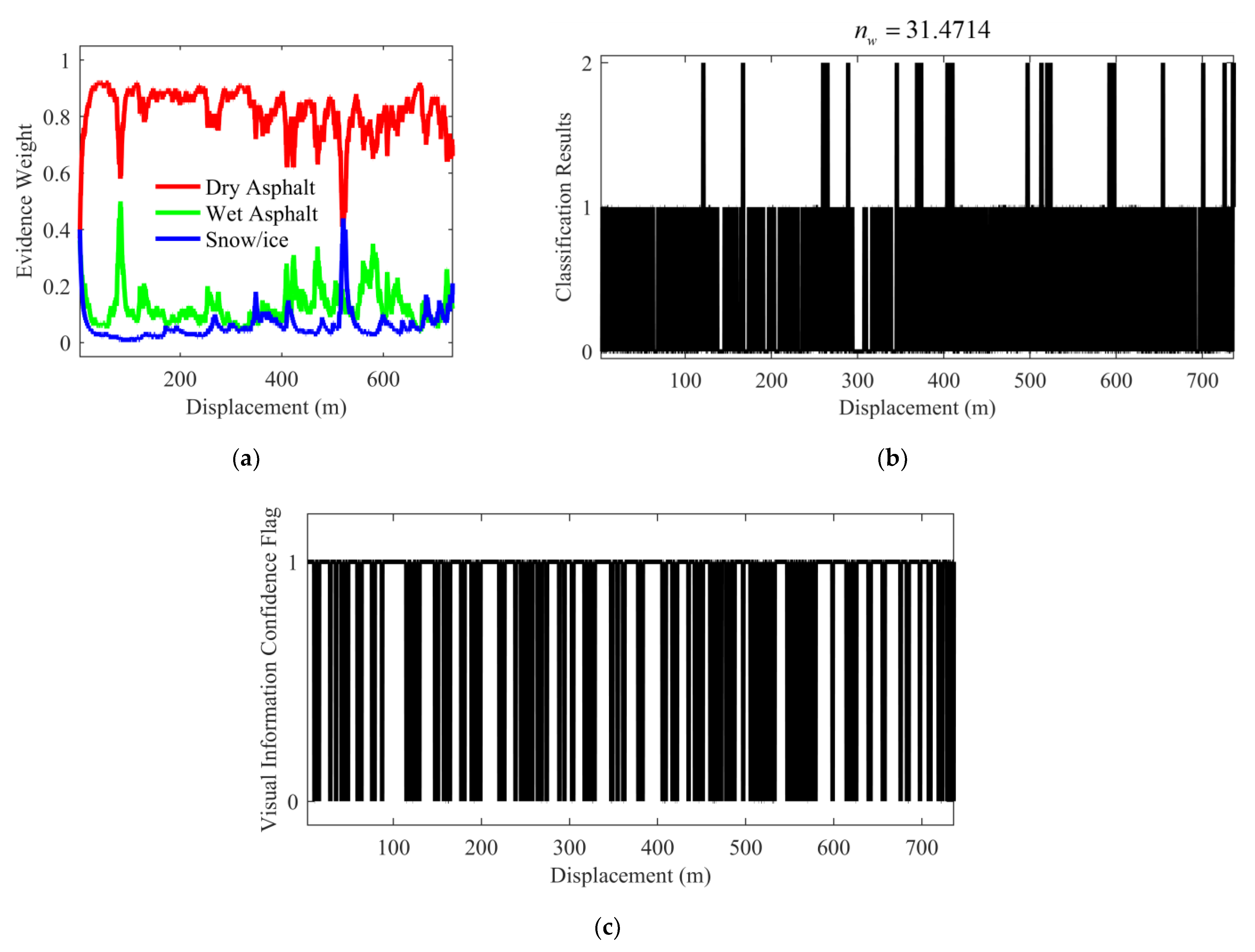
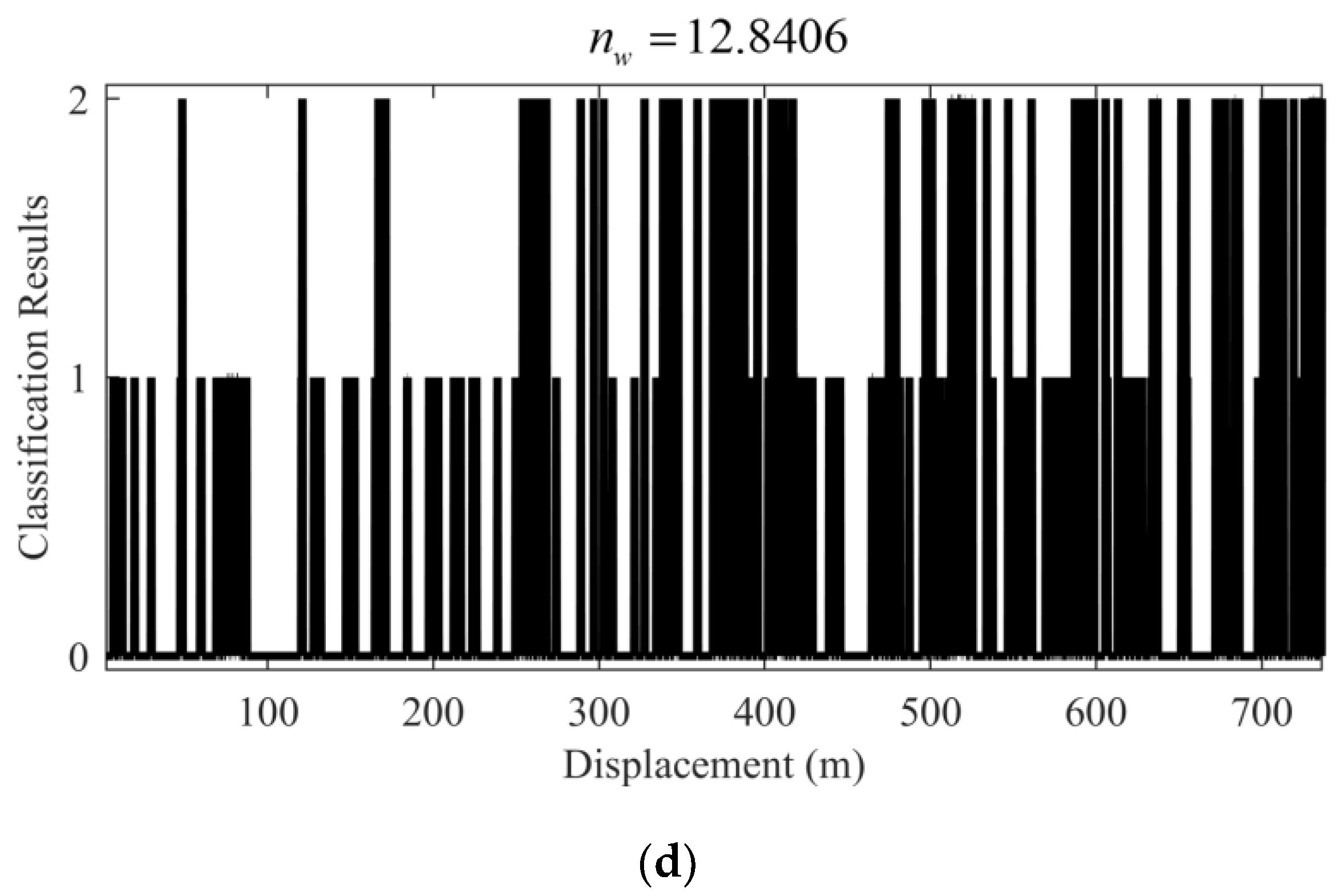
5.1.2. Test under the Scenario with Environmental Interference

Figure 14 shows the test results under the scenario with environmental interference. It can be clearly seen from Figure 14 that the performance of both IFE and IE based on the voting strategy has been affected by environmental interference. It is worth noting that the performance of IE based on the voting strategy has dropped significantly, and the $n_w$ value is as high as 31.4714, while the $n_w$ value of the proposed IFE can still be maintained below 13. In addition, it can also be seen from the visual information confidence flag shown in Figure 14c that most of the IFE classification results corresponding to the flag “0” are misidentified. This shows that the proposed IFE can better screen the interference information to suppress the negative impact of the interference information on the subsequent fusion estimation system as much as possible.

In the example of the test results shown in Figure 15, the road feature extraction network based on multi-task learning can extract the road feature area without shadow coverage. In Figure 15e, it can be seen that the road shadow greatly interferes with the performance of the IE based on the voting strategy. The proposed IFE can better avoid the shadow area and output more accurate classification results.

5.1.3. Specific Test Results of IFE

The specific test results of IFE are summarized in the

Table 4. Specific Test results of IFE.

Scenarios	Methods	Average Incorrect Classification Results per 100 Consecutive Frames ${\mathit{n}}_{\mathit{w}}$
Normal	IE based on voting strategy [20]	21.6621
	IFE	1.5327
w/Interference	IE based on voting strategy [20]	31.4714
	IFE	12.8406

.

5.2. Performance Validation for DIFE

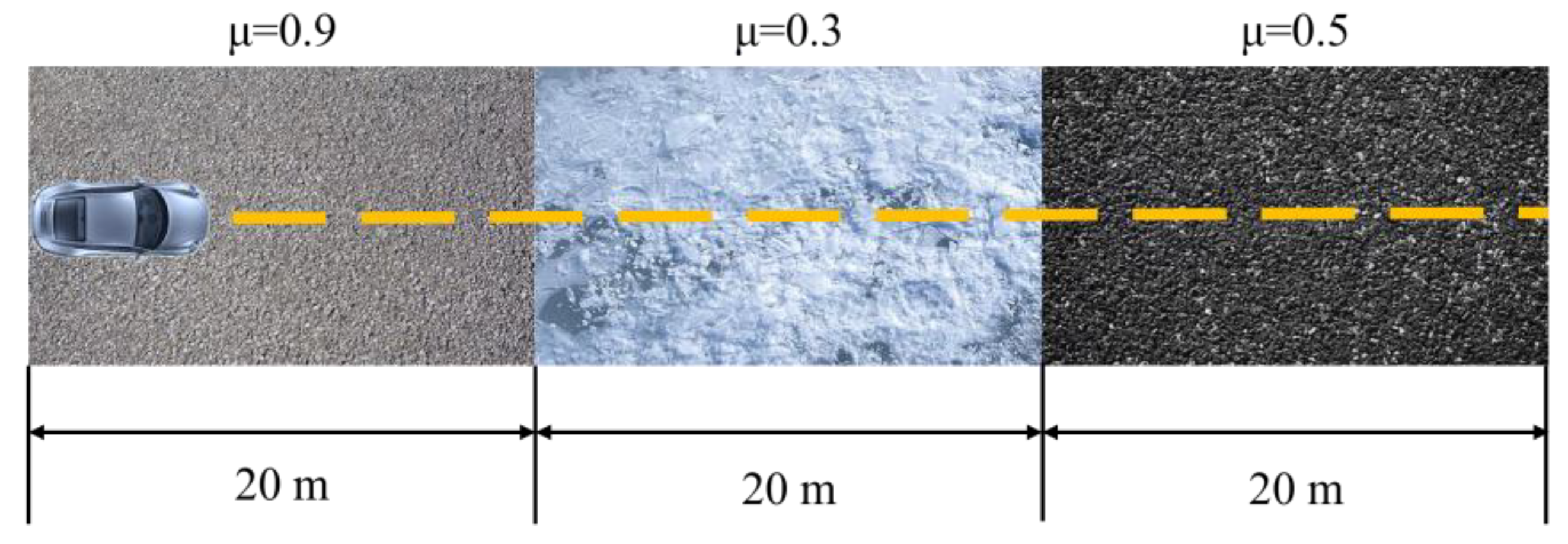
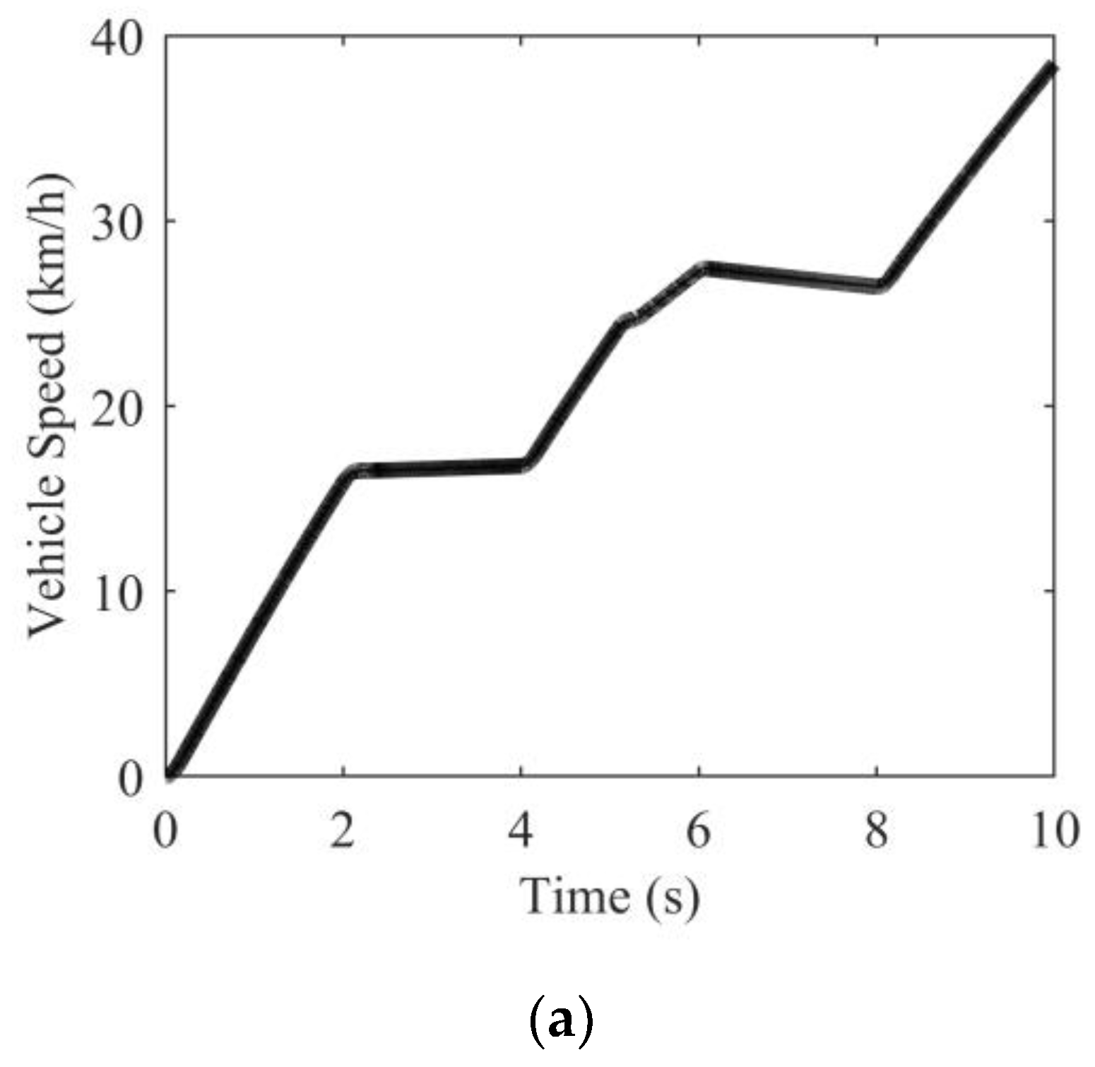
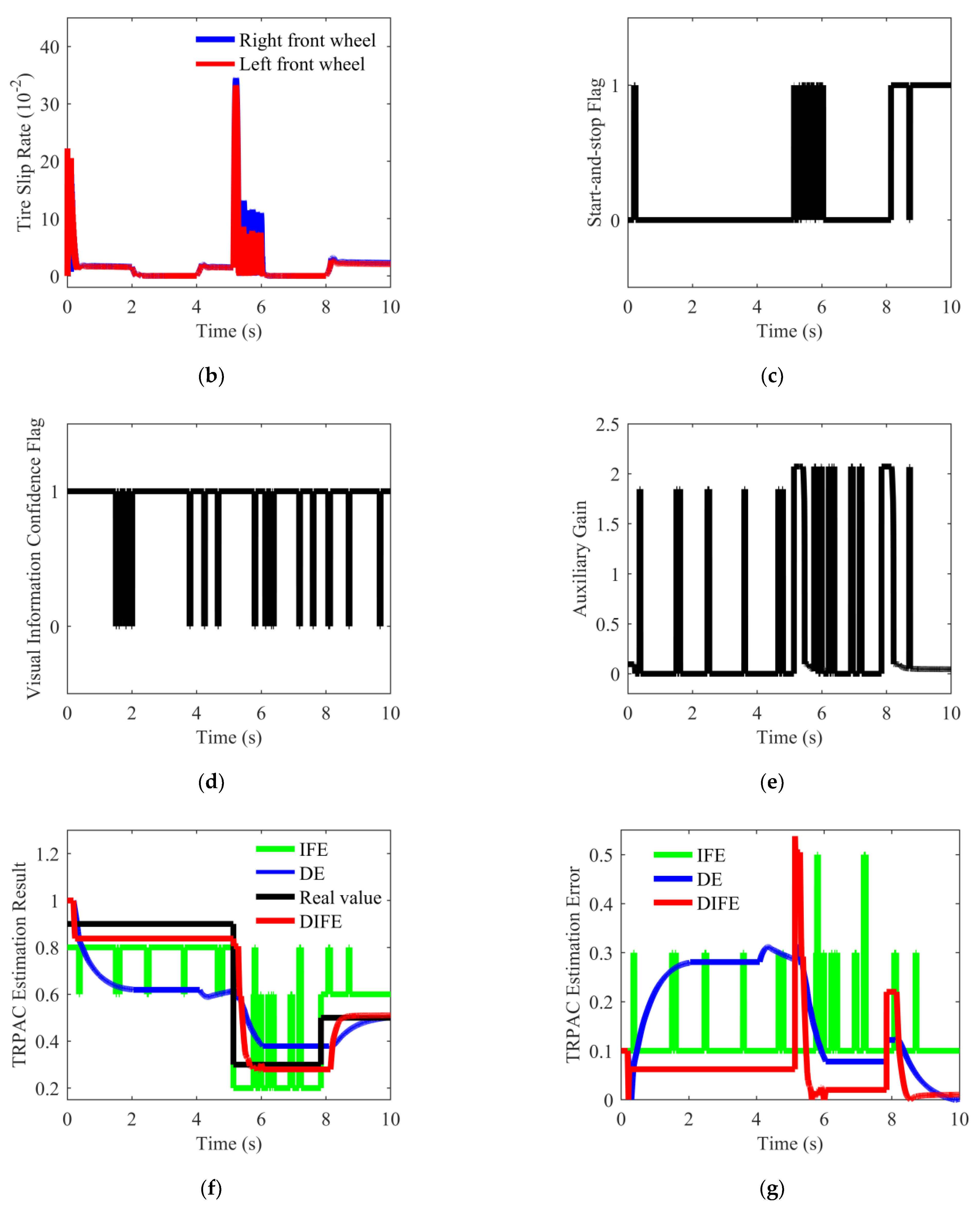
5.2.1. Simulation on Variable Friction Road

In order to verify the performance of the proposed fusion estimation method under variable friction road, the simulation condition shown in Figure 16 was designed. The TRPACs of the road were set to 0.9 (simulating a high-friction road), 0.3 (simulating a low-friction road), and 0.5 (simulating a middle-friction road). The road length of each road surface condition is 20 m. The vehicle was driven with pulsed acceleration maneuvers to simulate the intermittent road excitation obtained during real driving maneuvers. To test the robustness of the fusion estimator system under disturbances, the video data used for the simulation is noised based on the image data augmentation library [29]. The simulation result is shown in Figure 17.

It can be seen from Figure 17b that due to the acceleration of the vehicle from the start, the vehicle obtained a brief road excitation, but it was still insufficient. In the initial stage, both DE and DIFE started to work, but the underestimation of DE was more obvious. During the following 0.3–5.14 s, the estimated value of DIFE remained relatively stable, and the estimated value of DE changed slightly due to small road excitations. When the vehicle entered the low-friction road at around 5.14 s, the road excitation suddenly increased. Due to the discontinuity of road excitation, both DE and DIFE had different degrees of intermittent response. When the road excitation was sufficient, the auxiliary gain increased rapidly to assist the DIFE to converge quickly. It took DIFE approximately 0.5 s to converge to the real value, while DE converged slowly with a convergence time as high as 0.9 s. At about 7.85 s, the vehicle traveled to a middle-friction road. At this time, the vehicle was unpowered, and the road excitation was insufficient. Therefore, both DE and DIFE were unresponsive. At approximately 8.14 s, DE and DIFE started to work as the motor torque increased. After DIFE is triggered, the auxiliary gain increases rapidly to make the estimated value converge quickly, while it takes DE approximately 1.5 s to converge to near the real value.

In addition, it is worth noting that, thanks to the visual information confidence flag shown in Figure 17d, DIFE can better avoid the influence of incorrect IFE estimation results on the fusion estimation system. It can be seen that DIFE has obvious advantages over DE, the convergence time is about 0.5 s, and the steady-state convergence error can be maintained within 0.02 in slippery road conditions (i.e., middle-friction road and low-friction road).

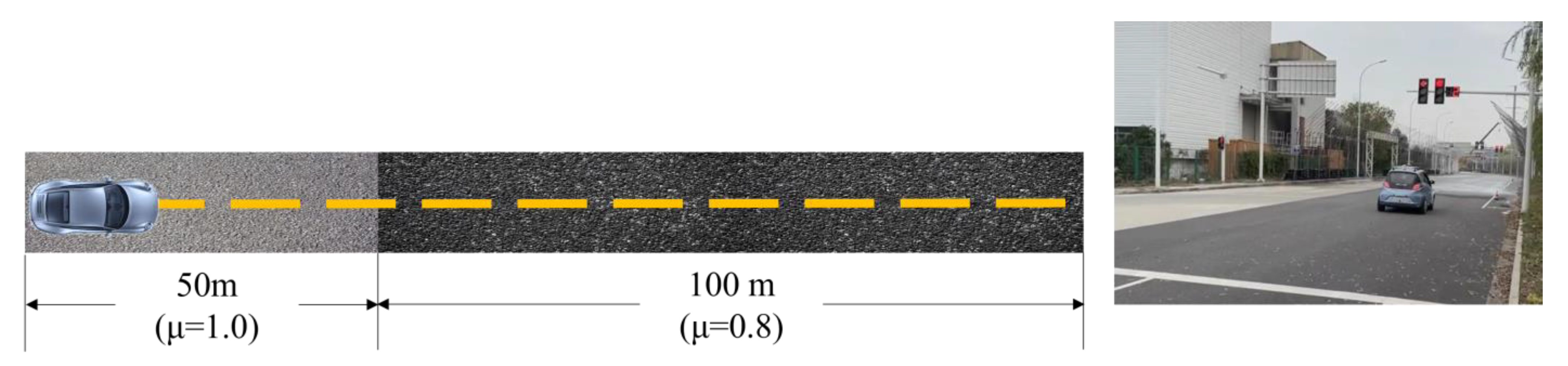
5.2.2. Vehicle Test on Variable Friction Road

As shown in Figure 18, the total length of the road for the vehicle test is 150 m, and the rain-fog simulation system was used to treat the road surface as wet and slippery. A BM-3 pendulum friction tester was used to test the TRPAC of the test road, where the TRPAC of the first 50 m was measured as 1.0 (dry asphalt road) and the TRPAC of the last 100 m was 0.8 (wet asphalt road). The vehicle started from a standstill, and the accelerator pedal was pulsed to create intermittent road excitation throughout the driving process. The vehicle test result is shown in Figure 19.

The road excitation for the test case shown in Figure 19 was discontinuous, thereby challenging the performance of the estimator. As shown in Figure 19f, the DE convergence was slow in the initial stage due to the influence of sensor noise at the time of 0–13.3 s. However, the visual information was used by DIFE in the initial stage, and the auxiliary gain increased rapidly, which made the convergence speed significantly faster than DE. This is because the road excitation was relatively limited, which caused the estimator to work for a short duration. Based on the auxiliary gain of visual information, DIFE could make better use of short-lived excitations, so that the estimated values of TRPAC were fully converged.

In the stage of 13.3–20 s, the convergence of DE was obviously delayed due to insufficient excitation, while DIFE can not only perceive road changes quickly, but also converge more smoothly in the steady-state stage, and the estimation error of DIFE was small. The steady-state estimation error of DIFE is within ±0.03, and the convergence time is within 0.4 s.

5.2.3. Specific Test Results of DIFE

The specific test results of DIFE are summarized in the

Table 5. Specific Test results of DIFE.

Condition	Methods	Steady-State Estimation Error	Convergence Time
Simulation	IFE	0.1~0.5	0.03 s
	DE	0.08	1.45~1.6 s
	DIFE	$\le$0.02	$\le$0.5 s
Vehicle test	IFE	0.2~0.4	0.03 s
	DE	>0.09	>4 s
	DIFE	$\le$0.03	$\le$0.4 s

.

6. Conclusions

In this paper, a TRPAC fusion estimation method considering model uncertainty is proposed to achieve fast and accurate estimation of TRPAC. The results achieved in this paper are as follows.

(1)

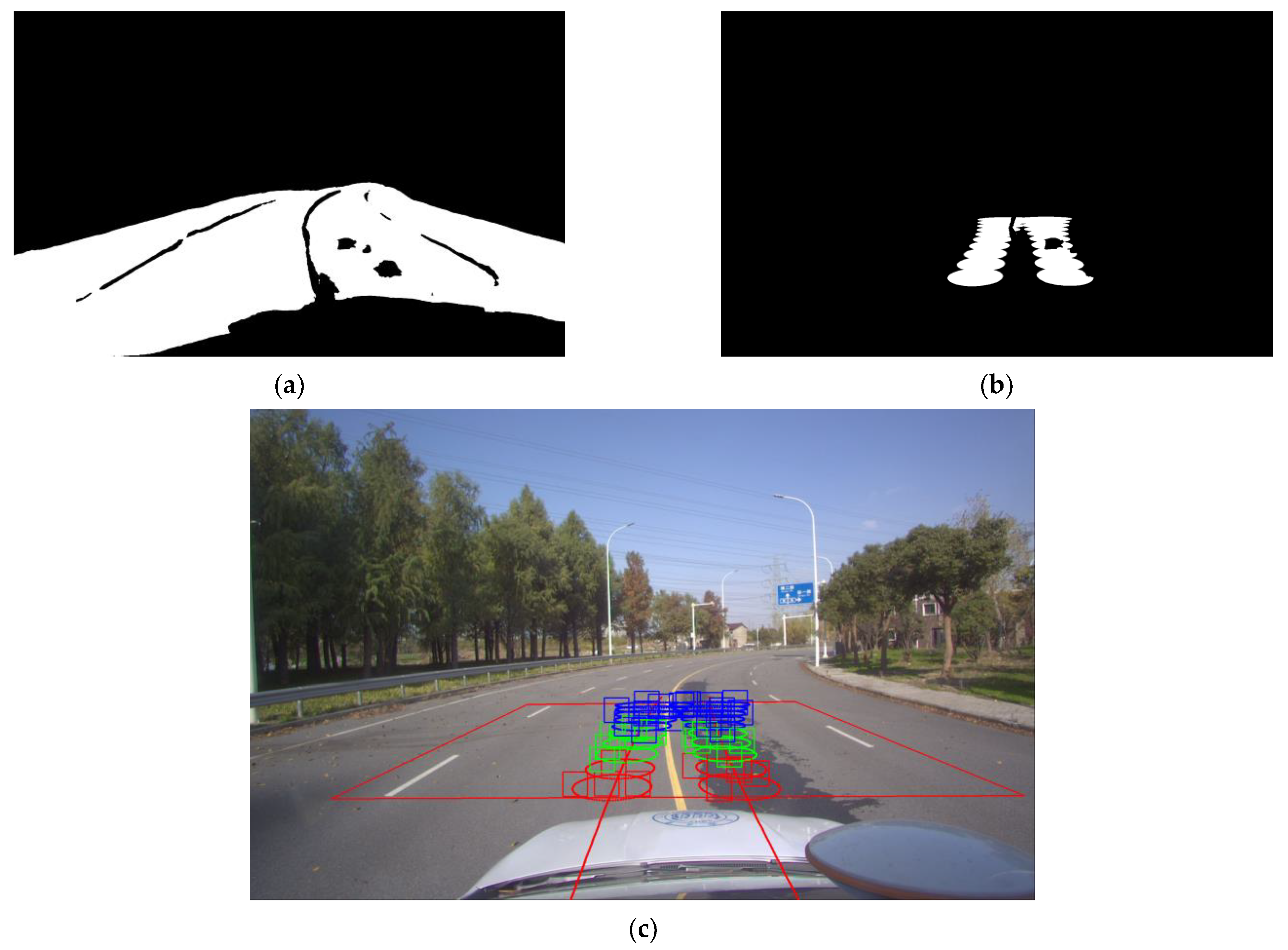
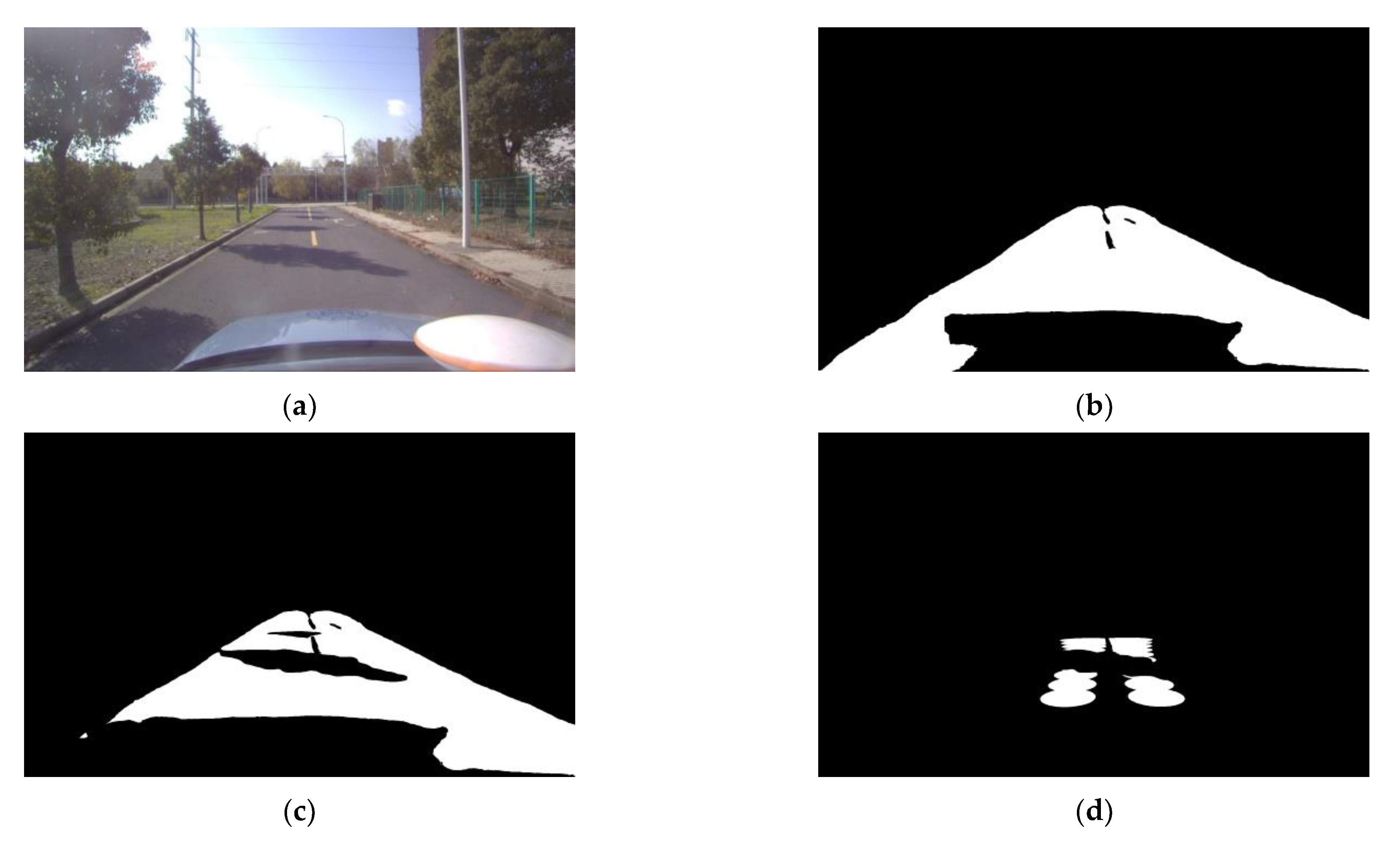
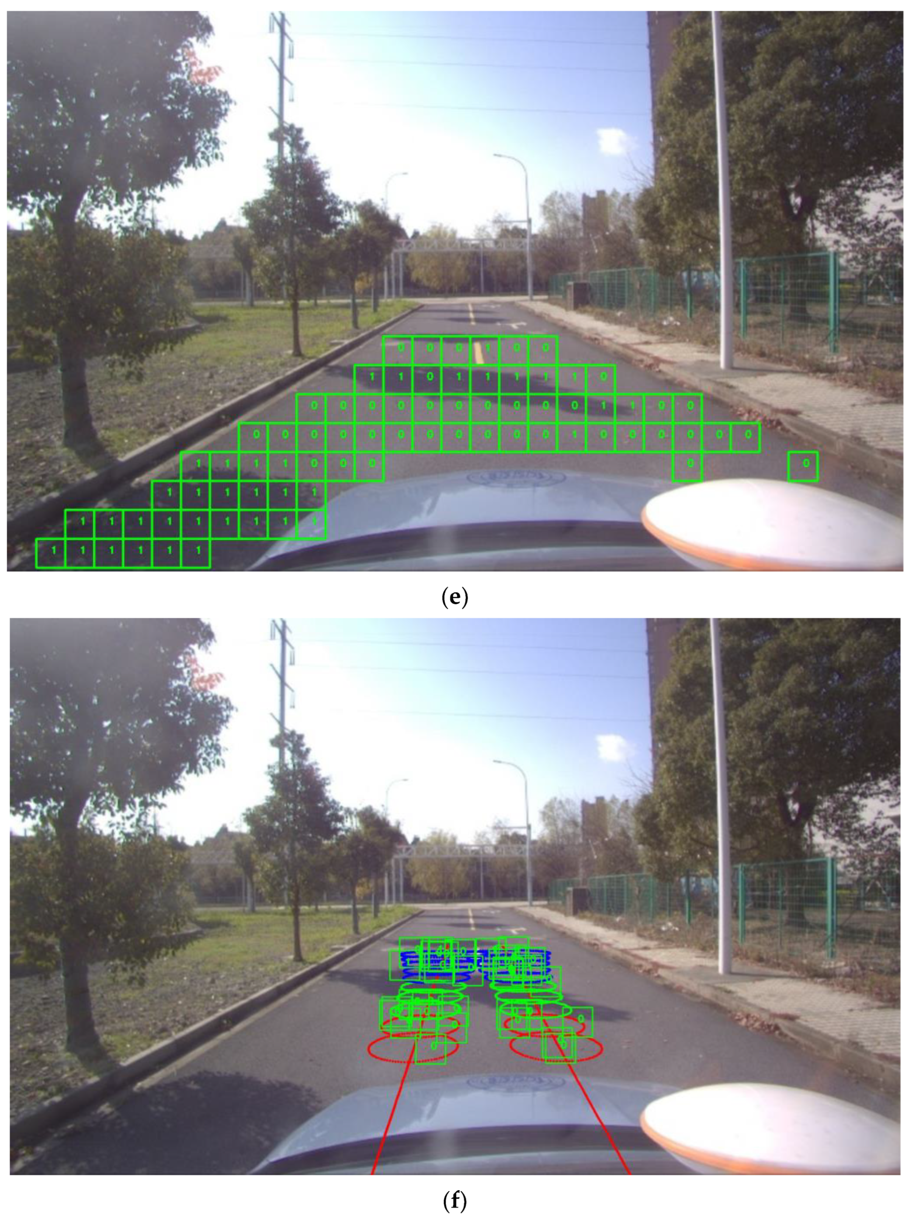
Considering common visual degradation factors, an IFE is proposed to achieve accurate classification of the road surface condition on which the vehicle will travel. The road image is segmented and classified in the road feature identification module to obtain road features without shadow coverage. Then, the ego-vehicle trajectory reckoning module is applied to extract the effective road area. Based on the fusion module, the candidate ROIs on the effective road area are fused to output the defined visual information confidence and classification results at the same time.

(2)

Based on gain scheduling theory, a DIFE considering the visual information confidence is designed to accelerate the convergence of DE while considering the uncertainty of visual information. In this way, the influence of incorrect IFE estimation results can be avoided as much as possible, and the accuracy of TRPAC estimation results can be ensured.

(3)

The performance of the IFE is verified in the vehicle tests under undisturbed and disturbed scenarios. The effectiveness of DIFE is verified in simulation and real vehicle experiments. The results show that the proposed DIFE has better estimation robustness and estimation accuracy than other single-source-based estimators. Moreover, the proposed DIFE can quickly respond to dangerous conditions such as sudden changes in the road surface, which is beneficial to the vehicle active safety system and intelligent transportation system.

References

1. Blundell, M.; Harty, D. The Multibody Systems Approach to Vehicle Dynamics, 2nd ed.; Elsevier: Amsterdam, The Netherlands, 2015; pp. 335–450. [Google Scholar]
2. Xue, W.; Zheng, L. Active Collision Avoidance System Design Based on Model Predictive Control with Varying Sampling Time. Automot. Innov. 2020, 3, 62–72. [Google Scholar] [CrossRef]
3. Cabrera, J.A.; Castillo, J.J.; Perez, J.; Velasco, J.M.; Guerra, A.J.; Hernandez, P. A procedure for determining tire-road friction characteristics using a modification of the magic formula based on experimental results. Sensors 2018, 18, 896. [Google Scholar] [CrossRef] [PubMed] [Green Version]
4. Zhang, X.; Xu, Y.; Pan, M.; Ren, F. A vehicle ABS adaptive sliding-mode control algorithm based on the vehicle velocity estimation and tyre/road friction coefficient estimations. Veh. Syst. Dyn. 2014, 52, 475–503. [Google Scholar] [CrossRef]
5. Faraji, M.; Majd, V.J.; Saghafi, B.; Sojoodi, M. An optimal pole-matching observer design for estimating tyre-road friction force. Veh. Syst. Dyn. 2010, 48, 1155–1166. [Google Scholar] [CrossRef]
6. Beal, C.E. Rapid Road Friction Estimation using Independent Left/Right Steering Torque Measurements. Veh. Syst. Dyn. 2020, 58, 377–403. [Google Scholar] [CrossRef]
7. Hu, J.; Rakheja, S.; Zhang, Y. Real-time estimation of tire-road friction coefficient based on lateral vehicle dynamics. Proc. Inst. Mech. Eng. Part D J. Automob. Eng. 2020, 234, 2444–2457. [Google Scholar] [CrossRef]
8. Shao, L.; Jin, C.; Lex, C.; Eichberger, A. Robust road friction estimation during vehicle steering. Veh. Syst. Dyn. 2019, 57, 493–519. [Google Scholar] [CrossRef]
9. Shao, L.; Jin, C.; Eichberger, A.; Lex, C. Grid Search Based Tire-Road Friction Estimation. IEEE Access 2020, 8, 81506–81525. [Google Scholar] [CrossRef]
10. Liu, W.; Xiong, L.; Xia, X.; Lu, Y.; Gao, L.; Song, S. Vision-aided intelligent vehicle sideslip angle estimation based on a dynamic model. IET Int. Transp. Syst. 2020, 14, 1183–1189. [Google Scholar] [CrossRef]
11. Almazan, E.J.; Qian, Y.; Elder, J.H. Road Segmentation for Classification of Road Weather Conditions. In Proceedings of the Computer Vision—ECCV 2016. 14th European Conference: Workshops, Cham, Switzerland, 8–16 October 2016. [Google Scholar]
12. Leng, B.; Jin, D.; Xiong, L.; Yu, Z. Estimation of tire-road peak adhesion coefficient for intelligent electric vehicles based on camera and tire dynamics information fusion. Mech. Syst. Signal Process. 2021, 150, 1–15. [Google Scholar] [CrossRef]
13. Wang, S.; Kodagoda, S.; Shi, L.; Wang, H. Road-Terrain Classification for Land Vehicles: Employing an Acceleration-Based Approach. IEEE Veh. Technol. Mag. 2017, 12, 34–41. [Google Scholar] [CrossRef]
14. Roychowdhury, S.; Zhao, M.; Wallin, A.; Ohlsson, N.; Jonasson, M. Machine Learning Models for Road Surface and Friction Estimation using Front-Camera Images. In Proceedings of the 2018 International Joint Conference on Neural Networks, Rio de Janeiro, Brazil, 8–13 July 2018. [Google Scholar]
15. Cheng, L.; Zhang, X.; Shen, J. Road surface condition classification using deep learning. J. Visual Commun. Image Represent. 2019, 64, 102638. [Google Scholar] [CrossRef]
16. Du, Y.; Liu, C.; Song, Y.; Li, Y.; Shen, Y. Rapid Estimation of Road Friction for Anti-Skid Autonomous Driving. IEEE Trans. Intell. Transp. Syst. 2020, 21, 2461–2470. [Google Scholar] [CrossRef]
17. Peng, L.; Wang, H.; Li, J. Uncertainty Evaluation of Object Detection Algorithms for Autonomous Vehicles. Automot. Innov. 2021, 4, 241–252. [Google Scholar] [CrossRef]
18. Chen, L.; Luo, Y.; Bian, M.; Qin, Z.; Luo, J.; Li, K. Estimation of tire-road friction coefficient based on frequency domain data fusion. Mech. Syst. Sig. Process. 2017, 85, 177–192. [Google Scholar] [CrossRef]
19. Svensson, L.; Torngren, M. Fusion of Heterogeneous Friction Estimates for Traction Adaptive Motion Planning and Control. In Proceedings of the 2021 IEEE International Intelligent Transportation Systems Conference, Indianapolis, IN, USA, 19–22 September 2021. [Google Scholar]
20. Jin, D.; Leng, B.; Yang, X.; Xiong, L.; Yu, Z. Road Friction Estimation Method Based on Fusion of Machine Vision and Vehicle Dynamics. In Proceedings of the 31st IEEE Intelligent Vehicles Symposium, Las Vegas, NV, USA, 19 October–13 November 2020. [Google Scholar]
21. Tian, C.; Leng, B.; Hou, X.; Huang, Y.; Zhao, W.; Jin, D.; Xiong, L.; Zhao, J. Robust Identification of Road Surface Condition Based on Ego-Vehicle Trajectory Reckoning. Automot. Innov. 2022, 1–12. [Google Scholar] [CrossRef]
22. Zhang, X.; Zhou, X.; Lin, M.; Sun, J. ShuffleNet: An Extremely Efficient Convolutional Neural Network for Mobile Devices. In Proceedings of the 31st Meeting of the IEEE/CVF Conference on Computer Vision and Pattern Recognition, Salt Lake City, UT, USA, 18–22 June 2018. [Google Scholar]
23. Hullermeier, E.; Waegeman, W. Aleatoric and epistemic uncertainty in machine learning: An introduction to concepts and methods. Mach. Learn. 2021, 110, 457–506. [Google Scholar] [CrossRef]
24. Guo, C.; Pleiss, G.; Sun, Y.; Weinberger, K.Q. On calibration of modern neural networks. In Proceedings of the 34th International Conference on Machine Learning, Sydney, Australia, 6–11 August 2017. [Google Scholar]
25. Cubuk, E.D.; Zoph, B.; Mane, D.; Vasudevan, V.; Le, Q.V. Autoaugment: Learning augmentation strategies from data. In Proceedings of the 32nd IEEE/CVF Conference on Computer Vision and Pattern Recognition, Long Beach, CA, USA, 16–20 June 2019. [Google Scholar]
26. Chen, H.; Wang, X.; Wang, J. A Trajectory Planning Method Considering Intention-aware Uncertainty for Autonomous Vehicles. In Proceedings of the 2018 Chinese Automation Congress, Xi’an, China, 30 November–2 December 2018. [Google Scholar]
27. Peniak, P.; Bubenikova, E.; Kanalikova, A. The redundant virtual sensors via edge computing. In Proceedings of the 26th International Conference on Applied Electronics, Pilsen, Czech Republic, 7–8 September 2021. [Google Scholar]
28. Dempster, A.P. Upper and lower probabilities induced by a multivalued mapping. In Classic Works of the Dempster-Shafer Theory of Belief Functions; Yager, R.R., Liu, L., Eds.; Springer: Berlin, Germany, 2008; pp. 57–72. [Google Scholar]
29. Bian, M.; Chen, L.; Luo, Y.; Li, K. A dynamic model for tire/road friction estimation under combined longitudinal/lateral slip situation. In Proceedings of the SAE 2014 World Congress and Exhibition, Detroit, MI, USA, 8–10 April 2014. [Google Scholar]
30. Yu, F.; Lin, Y. Automotive System Dynamics, 2nd ed.; Mechanical Industry Press: Beijing, China, 2017; pp. 30–67. [Google Scholar]
31. Xia, X.; Xiong, L.; Sun, K.; Yu, Z.P. Estimation of maximum road friction coefficient based on Lyapunov method. Int. J. Automot. Technol. 2016, 17, 991–1002. [Google Scholar] [CrossRef]
Figure 1. Overall framework of the proposed estimation method considering model uncertainty. (“CAL” denoted as “calibrated”.)
Remotesensing 14 05583 g001
Figure 2. Road feature extraction network based on multi-task learning.
Remotesensing 14 05583 g002
Figure 3. The learning process of the temperature scaling factor. (a) Loss in learning process; (b) The temperature scaling factor in learning process.
Remotesensing 14 05583 g003
Figure 4. The reliability diagrams of the classification model before and after calibration. (a) Reliability diagram of the original model; (b) Reliability diagram of the calibrated model.
Remotesensing 14 05583 g004
Figure 5. Kinematic bicycle model.
Remotesensing 14 05583 g005
Figure 6. The reckoned trajectory and uncertainty distribution in the vehicle coordinate system.
Remotesensing 14 05583 g006
Figure 7. The reckoned trajectory and uncertainty distribution in the image coordinate system.
Remotesensing 14 05583 g007
Figure 8. Flow chart of candidate ROIs extraction in the confidence ellipse region.
Remotesensing 14 05583 g008
Figure 9. The extraction process of the candidate ROIs extraction method. (a) Drivable area mask after removing road shadow; (b) Confidence ellipse region mask after removing road shadow; (c) Candidate ROIs within each group of confidence ellipses.
Remotesensing 14 05583 g009
Figure 10. The spatial position relationship in the spatiotemporal transformation strategy.
Remotesensing 14 05583 g010
Figure 11. Fuzzy control surfaces. (a) Fuzzy control surface of the road excitation threshold to trigger the DIFE; (b) Fuzzy control surface of the auxiliary gain.
Remotesensing 14 05583 g011
Figure 12. Experimental test platform.
Remotesensing 14 05583 g012
Figure 13. Test results under the normal scenario (left front wheel). (a) Evidence weight distribution; (b) Classification results of the IE based on the voting strategy; (c) Visual information confidence flag of the IFE; (d) Classification results of the IFE. (“0”, “1” and “2” represent dry, wet and snow/ice asphalt road, respectively.).
Remotesensing 14 05583 g013
Figure 14. Test results under the scenario with environmental interference (left front wheel). (a) Evidence weight distribution; (b) Classification results of the IE based on the voting strategy; (c) Visual information confidence flag of the IFE; (d) Classification results of the IFE. (“0”, “1” and “2” represent dry, wet and snow/ice asphalt road, respectively.).
Remotesensing 14 05583 g014aRemotesensing 14 05583 g014b
Figure 15. Example of the test results under the scenario with environmental interference. (a) Input image with environmental interference; (b) Drivable area mask; (c) Drivable area mask after removing road shadow; (d) Confidence ellipse region mask after removing road shadow; (e) Classification results of the IE based on the voting strategy; (f) Classification results of the IFE. (“0”, “1” and “2” represent dry, wet and snow/ice asphalt road, respectively.).
Remotesensing 14 05583 g015aRemotesensing 14 05583 g015b
Figure 16. Simulation condition.
Remotesensing 14 05583 g016
Figure 17. Simulation result. (a) Vehicle speed; (b) Tire slip rate; (c) Start-and-stop flag of the DIFE; (d) Visual information confidence flag; (e) Auxiliary gain of the DIFE; (f) Estimation result of different estimators; (g) Estimation error of different estimators.
Remotesensing 14 05583 g017aRemotesensing 14 05583 g017b
Figure 18. Vehicle test condition.
Remotesensing 14 05583 g018
Figure 19. Vehicle test result. (a) Vehicle speed; (b) Tire slip rate; (c) Start-and-stop flag of the DIFE; (d) Visual information confidence flag; (e) Auxiliary gain of the DIFE; (f) Estimation result of different estimators; (g) Estimation error of different estimators.
Remotesensing 14 05583 g019aRemotesensing 14 05583 g019b