Deep-Learning-Based Feature Extraction Approach for Significant Wave Height Prediction in SAR Mode Altimeter Data

Abstract

Predicting sea wave parameters such as significant wave height (SWH) has recently been identified as a critical requirement for maritime security and economy. Earth observation satellite missions have resulted in a massive rise in marine data volume and dimensionality. Deep learning technologies have proven their capabilities to process large amounts of data, draw useful insights, and assist in environmental decision making. In this study, a new deep-learning-based hybrid feature selection approach is proposed for SWH prediction using satellite Synthetic Aperture Radar (SAR) mode altimeter data. The introduced approach integrates the power of autoencoder deep neural networks in mapping input features into representative latent-space features with the feature selection power of the principal component analysis (PCA) algorithm to create significant features from altimeter observations. Several hybrid feature sets were generated using the proposed approach and utilized for modeling SWH using Gaussian Process Regression (GPR) and Neural Network Regression (NNR). SAR mode altimeter data from the Sentinel-3A mission calibrated by in situ buoy data was used for training and evaluating the SWH models. The significance of the autoencoder-based feature sets in improving the prediction performance of SWH models is investigated against original, traditionally selected, and hybrid features. The autoencoder–PCA hybrid feature set generated by the proposed approach recorded the lowest average RMSE values of 0.11069 for GPR models, which outperforms the state-of-the-art results. The findings of this study reveal the superiority of the autoencoder deep learning network in generating latent features that aid in improving the prediction performance of SWH models over traditional feature extraction methods.

1. Introduction

Wave conditions are important parameters in coastal engineering and the research of maritime processes. Wave conditions such as wave height and wind speed may assist in optimizing shipping routes and harvesting times of aquaculture farms. Wave height plays a crucial influence in energy extraction from waves, sediment movement, harbor design, and soil erosion. For any practical applications, long-term observed data are necessary. Methods for determining wave heights include field measurements, theoretical research, and numerical simulation. In most of these instances, however, there will be no long-term measurements, making wave height prediction vital.

Recently, satellite-based remote sensing systems including electro-optical, microwave radiometers, Synthetic Aperture Radar, and altimeters have been providing tremendous amounts of data about earth. Satellite data collection and processing is being used to significantly help to make operational decisions in many challenging environmental problems. For ocean observation from space, satellite imaging systems have demonstrated their capability to provide ocean wave spectra at high spatial resolution [1,2,3]. The Wave Mode (WM) has been specifically adopted by Envisat, ERS-1/2, and Sentinel-1A/B SARs to provide information on ocean waves in open ocean [4,5,6,7].

Traditionally, SWH retrieval schemes in satellite imagery can be classified into three categories as described in this section. The first group of algorithms depends on integrating the directional ocean wave spectrum estimated from the SAR spectrum. These methods require wind information or a first guess for the wave spectra [8,9,10,11]. Given that the relation between the wave spectrum and the SAR spectrum is nonlinear [12], and that it is not possible to predict the wave height below a certain frequency, estimation of wave height using this scheme is incomplete [12].

The second group includes empirical algorithms that have emerged since the 2000s. Empirical models can estimate SWH directly from features computed from SAR images and/or SAR spectra and do not require prior wave/wind information as in the first scheme. An example of these models that estimates significant wave height is the C-band WAVE algorithm called “CWAVE”. The original CWAVE algorithm has two versions, one that uses a mean and variance of image intensity (the base model) and one that adds 20 variables calculated from the image spectrum (the full-spectrum model) [12]. Many versions were developed for the CWAVE models such as the CWAVE_ERS for ERS-2 wave mode [13], CWAVE_ENV for Envisat wave mode [14], and other empirical Hs retrieval attempts for SAR data provided by Sentinel-1A [15,16], Radarsat-2 [17,18], and TerraSAR-X [19].

In the third category, various machine learning (ML) algorithms are employed for the purpose of wave parameters estimation. Machine and deep learning techniques have proven high prediction performance in several life fields. For instance, machine learning has been used for the medical diagnosis of many diseases [20,21,22,23], cyberbullying detection [24], environmental monitoring [25], augmentation of turbulence models [26], management of vegetated water resources [27,28], and in other applications. In oceanography and Earth sciences, ML has a diverse range of real-time applications. The primary applications of machine learning in oceanography include ocean weather and climate prediction, wave modeling, SWH, and wind speed predictions in regular sea state conditions [29,30] and in complex sea state conditions [29,31,32]. For instance, the study in [29] developed an ensemble of neural networks for the prediction of significant wave height from satellite images in an offshore region of a wind farm. The study by Stefanakos [31] integrated the Fuzzy Inference System with the Adaptive Network-based Fuzzy Inference System to predict wind and SWH parameters from a nonstationary wave parameters time series. Classical ML algorithms were used for wave height/wind speed estimation in the study by Stopa and Mouche [33], in which they implemented the CWAVE using a shallow feed-forward neural network using SAR images. They tested the full-spectrum model and the base model, and experimented with a few other parameters in the base model [33]. Collins et al. in [18] implemented the base and full-spectrum CWAVE models as neural networks and used Radarsat-2 Fine Quad data. They trained and tested the networks using buoy observations and investigated as well the effects of incidence angle and polarization. The common conclusion among the aforementioned studies is that neural networks extend the ability of retrieving the wave parameters using SAR images under a large range of environmental conditions in which SWH estimation is challenging. Although the results of the aforementioned study are promising, the approach of predicting SWH from satellite imagery itself is complicated and tedious.

For more than 30 years, satellite radar altimeters have provided comprehensive coverage of wind speed and significant wave height [34]. Numerous applications have made use of these data, such as offshore engineering design, numerical model validation, wind and wave climatology, and the analysis of long-term trends in oceanographic wind speed and wave height. However, the use of altimeter data for modeling SWH received little attention in the literature. Altimeter data provide several SWH and wind-speed-related parameters. The significance of these parameters for the prediction of SWH has not yet been investigated in the literature. Nevertheless, a single study has been found to utilize some altimeter features in the context of SWH prediction. The study of Quach et al. [35] integrated features from satellite altimeter data with a number of features that were derived from the modulation spectra of SAR images and developed a deep-learning-based prediction model for SWH. Their results show an improved prediction performance using their proposed method. Studies in the literature used other dataset types for predicting SWH. The majority of studies used buoy measurements for modeling SWH [32,36,37], while some recent studies used satellite imagery and extracted image features and used them for SWH prediction [12,14,29]. Only few papers have utilized altimeter data features for SWH forecasting [35]. The investigation of the significance of the entire set of features in altimeter data for SWH prediction is considered a gap in the literature. Motivated to fill this research gap, in this study, we propose a new framework to investigate the significance of altimeter data features in modeling SWH. Within this framework, a deep-learning-based feature extraction approach is introduced to extract significant features from SAR mode satellite altimeter data. The autoencoder deep learning neural network is utilized to extract latent features from the altimeter data. The autoencoder network has the capability to map the original input feature into an abstract set of significant latent features. Two traditional feature extraction approaches are utilized as well to extract extra features: the Pearson Correlation Coefficient (PCC) Analysis and the PCA. Several hybrid feature sets are then formed by fusing traditionally extracted and deep-learning-derived features. The feature sets are used for modeling SWH individually. This study proposes a novel hybrid approach for extracting significant features from altimeter data for SWH prediction. The deep learning autoencoder neural network was utilized, separately, and hybridized with other traditional feature extraction methods uniquely in this study for the prediction of significant wave height. To the best of our knowledge, no research has used autoencoders for SWH prediction in satellite data. Moreover, the hybrid combination of the (autoencoder–PCA) has not been presented in the literature for wave parameter prediction to data. The main contributions of the present study are listed as follows:

• Proposal of a new hybrid deep-learning-based approach for extracting features from SAR mode satellite altimeter data.
• Proposal of a new framework to investigate the significance of altimeter data-driven features for SWH prediction.
• Utilization of autoencoder deep learning neural network to extract latent features from the altimeter data.
• Generation of several feature sets composed of the original data features, traditionally extracted features, deep learning-derived features, and hybrid combinations from them.
• Utilization of the generated feature sets to model SWH using the Gaussian Process Regression and Neural Network Regression algorithms and evaluate the prediction performance.
• Comparing the prediction performance of the SWH models trained using the basic and hybrid feature sets.
• Evaluation of the significance of the proposed features using hypothesis testing.

The paper is structured as follows: Section 2 describes the dataset used in this work, Section 3 presents the used methods, Section 4 discusses the obtained results, and Section 5 concludes the work.

2. Dataset

The used dataset is satellite records of significant wave height and wind speed measured by the SENTINEL-3A altimeter. Sentinel-3A is an Earth observation satellite specialized to oceanography. It is the first of four Sentinel-3 satellites planned as part of the Copernicus Program. On 16 February 2016, the European Space Agency launched the Sentinel-3A satellite to measure sea surface topography, temperature, and color with high accuracy and dependability to support ocean forecasting systems, as well as environmental and climate monitoring [38]. SAR Radar Altimeter (SRAL) of SENTINEL-3A SLAR is a new-generation altimeter that operates in Synthetic Aperture Radar (SAR) mode at all times [39]. SAR mode is the optimum mode for data recording over open ocean surface since it is designed to achieve high along-track resolution over generally flat surfaces [39]. A summary of Sentinel-3A altimeter operating characteristics is provided in

Table 1. Summary of Sentinel-3A altimeter operating characteristics [40].

Altimetry Instrument	Revisit Time	Inclination	Frequency	Frequency Band	Altitude	Latitude Coverage	Life Time
SRAL	27 days	98.650	13.575 GHz 5.41 GHz	KU C	814.5 km	−78 to 81	2016–ongoing

. Altimetry instrument, exact repeat mission period, orbit parameters such as inclination and altitude, antenna properties such as frequency and frequency band, latitude coverage, and operational time for Sentinel-3A are depicted in Table 1.

The dataset used in this study is a subset of the IMOS (Integrated Marine Observing System, Battery Point, Australia) Surface Waves Sub-Facility Altimeter Wave/Wind database publicly available through the Australian Ocean Data Network portal (AODN: https://portal.aodn.org.au/, accessed on 15 August 2022). The IMOS dataset is a large archive of global significant wave height and wind speed records measured by 13 satellite altimeters over 33 years from 1985 to 2018 [34]. The altimeters of GEOSAT, ERS-1, TOPEX, ERS-2, GFO, JASON-1, ENVISAT, JASON-2, CRYOSAT-2, HY-2A, SARAL, JASON-3, and SENTINEL-3A were used to collect the SWH and wind speed measurements. Values of significant wave height and wind speed are derived from high-frequency altimeter data by fitting a functional form to the radar return from the ocean surface through the waveform retracking process. Altimeter data in this database were calibrated using a long-term high-quality wind speed and wave height database measured by in situ buoys from the National Oceanographic Data Center (NODC). Due to land and ice contamination, and the quality of the altimeter waveform received by the satellite, altimeter-generated Geophysical Data Records may contain data spikes. Therefore, quality flags were used to specify the goodness level of the data and aid in quality controlling it. The archive data contains a series of data flags defined as 1, 2, 3, 4, and 9; these flags represent ‘Good data’, ‘Probably good data’, ‘Hardware error, ‘Bad data’, and ‘Missing data’, respectively [34]. In this study, only good quality and probably good data are used.

Data of two geographical positions were selected for this study; throughout the paper, the first position is referred to as ‘P0’, while the second location is referred to as ‘P1’. Position P0 is located at 0° latitude and 0° longitude (0°N 0°E), which is a point in the Atlantic Ocean. This point is called the Null Island and is located where the prime meridian meets the equator. The Null Island lies in international waters in the Atlantic Ocean, about 600 km off the coast of West Africa in the Gulf of Guinea [41]. Position P1 is located at 0° latitude and 1° longitude (0°N 1°E), which is located as well in the Atlantic Ocean. For P0, data records were acquired for the period from 26 March 2016 at 09:57:02 Z′ to 11 July 2018 at 09:57:30 Z′. The data file for P0 contains 1008 records. The data of position P1 contain 1033 entries and were acquired from 3 March 2016 at 09:53:25 Z′ to 15 July 2018 at 09:53:46 Z′. For each position, the data file contains 26 variables, as depicted in

Table 2. Data variables’ names and their definitions [34].

Feature Name	Feature Description
TIME	Time of data acquisition provided as a number referenced to 1985-01-01, 00:00:00 UTC.
LATITUDE	The angle that is created when a vector that is perpendicular to an ellipsoidal surface is drawn from a point on the surface.
LONGITUDE	A type of geographic coordinate that indicates the position of a point on the surface of the Earth with relation to the east–west axis.
BOT_DEPTH	Ocean floor depths underwater.
DIST2COAST	Distance from the coast.
SIG0_C	Backscatter coefficient for C-band altimetry.
SIG0_C_quality_control	Backscatter coefficients quality flags in C-band altimetry.
SIG0_C_num_obs	The number of valid C-band altimetry backscatter coefficient measurements at 20 Hz that make up the 1 Hz measurement.
SIG0_C_std_dev	The 1 Hz measurement is comprised of the standard deviation of the data that make up the 20 Hz C-band altimetry backscatter coefficient.
SIG0_KU	Coefficient of backscatter for Ku band altimetry.
SIG0_KU_quality_control	Quality flags of backscatter coefficient in Ku-band altimetry.
SIG0_KU_num_obs	Amount of all valid 20 Hz Ku-band altimetry backscatter coefficient data used to calculate the 1 Hz value.
SIG0_KU_std_dev	The 1 Hz measurement is based on the standard deviation of the data for the 20 Hz Ku-band altimetry backscatter coefficient.
SWH_C	The height of a significant wave, as measured by uncalibrated C-band altimetry.
SWH_C_quality_control	Significant wave height quality flag for C-band altimetry.
SWH_C_num_obs	Significant wave height values taken at 20 Hz by C-band altimetry and converted to a 1 Hz scale.
SWH_C_std_dev	Standard deviation of significant wave height measured at 1 Hz using C-band altimetry, based on data collected at 20 Hz.
SWH_KU	Significant wave height as measured by uncalibrated Ku-band altimetry.
SWH_KU_CAL	The significant wave height was calibrated using the Ku-band altimetry.
SWH_KU_quality_control	Flag indicating the quality of the Ku-band altimetry significant wave height data.
SWH_KU_num_obs	The number of valid Ku-band altimetry readings of significant wave height that were used to construct the 1 Hz measurement.
SWH_KU_std_dev	The standard deviation of the significant wave height data collected at 20 Hz by Ku-band altimetry and used to construct the 1 Hz measurement.
UWND	Modeling zonal wind speed using ECMWF.
VWND	Modeling meridional wind speed using ECMWF.
WSPD	Wind speed derived from wind function alone and not calibrated.
WSPD_CAL	The wind speed was calibrated based on the wind function.

. The records are binned into bins of 1° by 1°. Full data resolution is provided within each bin for the corresponding latitude and longitude of every 1 Hz measurement [34].

3. Methods

In this section, the proposed framework and methods used for feature extraction are presented. Regression algorithms used for SWH modeling and performance evaluation methods are also provided.

3.1. Proposed Framework

In this study, the proposed framework introduces a hybrid approach for extracting the significant features for the prediction of SWH from altimeter data. This hybrid approach combines the features generated by three feature extraction techniques. The Pearson Correlation Analysis, Principal Component Analysis algorithms, and Sparse Autoencoder deep neural network are utilized to extract the most significant attributes from the input features. Multiple hybrid feature combinations are introduced and examined for modeling SWH using Gaussian Process Regression and Neural Network Regression. The proposed framework is composed of four phases: the data preprocessing phase, feature sets formation phase, SWR modeling phase, and model evaluation and testing phase. In the data preprocessing phase, multiple preprocessing steps are conducted to prepare the data for the feature sets formation phase. In the feature sets formation phase, a number of basic and hybrid feature sets are created from the input data. Basic sets include the ALL-Set, PCC-Set, PCA-Set, and AUT-Set-N. The ALL-Set is composed of all features in the dataset excluding the response variable to be predicted, namely SWH. Pearson Correlation Coefficients between input features and the response variable are thresholded to select the features encompassed in the PCC-Set. Features in the PCA-Set are generated by the PCA algorithm with 95% variance. Autoencoder-driven features are generated by training a sparse autoencoder neural network by all input features and extracting a specified number of latent space features from the encoder. Up to three latent features are derived by the autoencoder network and formed three autoencoder-driven feature sets, namely AUT-Set-1, AUT-Set-2, and AUT-Set-3. Multiple hybrid feature sets are further formed using various combinations of the PCC, PCA, and AUT feature sets. Hybrid sets include the HAT-N and HCAT-N sets. The composition of theses sets is elaborated in the Results section. In the SWH modeling phase, the training dataset is used for training a number of Gaussian Process regression and Neural Network regression models. The regression models are validated using a 5-cross validation scheme and tested on a holdout test set in the final model evaluation and testing phase. The prediction performance of the SWH models trained on the hybrid feature sets are compared with that trained by the basic PCC, PCA, and autoencoder feature sets, as well as all input features set. The proposed framework is presented in Figure 1.

3.2. Data Preprocessing

In this phase, multiple data preprocessing steps are conducted to prepare the data for the feature sets formation phase, as shown in Figure 2. The target/response variable to be predicted in this work is SWH. The remaining variables are preprocessed to prepare the input features that will be used for predicting the target. In this study, quality control flags for the SWH and SIG0 are discarded, and the remaining features are divided into four categories: observing condition features, site related features, wind speed features, and measured features. The features under each category are depicted in

Table 3. Categorization of input features.

Observing Condition Features	Site Features	Measured Features		Wind Speed Features
		KU-Band Features	C-Band Features
TIME	DIST2COAST	SIG0_KU	SIG0_C	VWND
LATITUDE	BOT_DEPTH	SIG0_KU_std_dev	SIG0_C_std_dev	WSPD
LONGITUDE		SIG0_KU_num_obs	SIG0_C_num_obs	UWND
		SWH_KU_num_obs	SWH_C_num_obs	WSPD_CAL
		SWH_KU_std_dev	SWH_C_std_dev

. The measured features are further categorized according to the frequency band used for data acquisition into KU-band-related features and C-band features. The SRAL altimeter on Sentinel 3A uses the KU-band (13.575 GHz, bandwidth 350 MHz) for range measurements. However, it uses the C-band (5.41 GHz, bandwidth 320 MHz) for ionospheric correction [42]. This is achieved in the SAR acquisition mode by using bursts of 64 KU-band pulses surrounded by two C-band pulses [42]. Therefore, in this study, the SWH modeling was conducted using only the KU-band-measured features along with the other site and observing condition features.

In order to maintain close ranges of the input variables, the features are normalized to have unit standard deviation and zero mean, with the following exceptions. The latitude and longitude features are replaced by their sine and cosine values after converting them into angles in the range [0, 2π] rad. Features containing the number of observations are converted to discrete values in the range [0–3] by subtracting each entry by the feature’s maximum value. After data normalization, the dataset is subdivided into training and testing sets with 90:10 training to testing ratio.

3.3. Feature Sets Formation

In this phase, a number of basic and hybrid feature sets are generated and used to model the SWH. A number of feature extraction and reduction approaches were used to extract significant features from the input data. The Pearson Correlation Analysis, Principal Component Analysis, and the autoencoder deep neural network are used for feature extraction and selection. Three basic feature sets are formed using features extracted from the all-features set (ALL-Set) by these algorithms: PCC-Set, PCA-Set, and AUT-Sets. The feature formation phase is depicted in Figure 3.

3.3.1. Pearson Correlation Analysis

Pearson Correlation Analysis is an approach to find the linear correlation between two random variables. The Pearson correlation coefficient is considered a measure of dependency between two vectors. PCC between a pair of variables X and Y can be evaluated using Equation (1). PCC can take values in the range [−1, 1]. Absolute PCC values near 1 mean high linear dependency between variables, while values close to zero show low dependency.

$$\mathrm{PCC}=\frac{\mathrm{cov}\left(\mathrm{X},\mathrm{Y}\right)}{\sqrt[2]{\mathsf{\sigma }\left(\mathrm{X}\right)\mathsf{\sigma }\left(\mathrm{Y}\right)}}$$

(1)

where, $\mathsf{\sigma }\left(\mathrm{X}\right)$, $\mathsf{\sigma }\left(\mathrm{Y}\right)$ are the variance of X and Y, respectively, and $\mathrm{cov}\left(\mathrm{X},\mathrm{Y}\right)$ is the covariance matrix between X and Y.

In this study, Person Correlation Coefficients between input features and the response variable are computed and thresholded to select the features encompassed in the PCC-Set. The selection of the threshold value is data-dependent, as discussed in the Results section.

3.3.2. Principal Component Analysis

Principal component analysis, or PCA, is traditional data analysis approach that generates a series of the best linear approximations for a given dataset. It is considered the most widely used method for dimensionality reduction with minimum information loss [22,43,44]. In this research, the PCA is employed to extract a sequence of uncorrelated features, or principal components (PCs), from the altimeter observational data. The new PC features represent linear combinations of the input variables and comprise the major information contained in the original data. For data matrix Z with $m$ number of variables and $n$ number of samples given as $Z=\left(\begin{array}{ccc}{v}_{11} v_{21}& \cdots & v_{m1}\\ ⋮& \ddots & ⋮\\ v_{1n} v_{2n}& \cdots & v_{mn}\end{array}\right)$, the PCA algorithm could generate $\mathrm{k}$ uncorrelated features using linear combinations of the input variables. The principal components denoted as ${\mathrm{u}}_{1, }{ \mathrm{u}}_{2, }{ \mathrm{u}}_{3, },\dots .,{ \mathrm{u}}_{\mathrm{k} }$ are given in Equation (2), where $l_{\mathrm{ij}}$ is the linear combinations coefficient [44].

$$\{\begin{array}{c}{\mathrm{u}}_1=l_{11} v_1+l_{12} v_2+l_{13} v_3+\dots +l_{1\mathrm{m}} v_{\mathrm{m}}={\displaystyle {\displaystyle \sum }_{i=1}^m}{l}_{1\mathrm{i}} v_{\mathrm{i}}\\ {\mathrm{u}}_2=l_{21} v_1+l_{22} v_2+l_{23} v_3+\dots +l_{2\mathrm{m}} v_{\mathrm{m}}={\displaystyle {\displaystyle \sum }_{i=1}^m}{l}_{2\mathrm{i}} v_{\mathrm{i}}\\ .\\ .\\ .\\ {\mathrm{u}}_{\mathrm{k}}=l_{\mathrm{k}1} v_1+l_{\mathrm{k}2} v_2+l_{\mathrm{k}3} v_3+\dots +l_{\mathrm{km}} v_{\mathrm{m}}={\displaystyle {\displaystyle \sum }_{i=1}^m}{l}_{\mathrm{ki}} v_{\mathrm{i}}\end{array}$$

(2)

The principal components satisfy two conditions; the retrieved features (${\mathrm{u}}_1,{ \mathrm{u}}_2,{ \mathrm{u}}_3,\dots ,{ \mathrm{u}}_{\mathrm{k}}$) are uncorrelated, and the first principal component, ${\mathrm{u}}_1$, has the highest variance followed by ${\mathrm{u}}_2$, etc. The number of extracted features, PCs, is determined based on the Cumulative Percent Variance (CPV). CPV is used as a threshold to determine the $\mathrm{k}$ number of PCs that covers the required percent of information in the original data. The level of CPV is decided in advance. In this work, the PCA-Set includes the principal components generated by the PCA algorithm with a CPV of 95%.

3.3.3. Autoencoder Neural Network

An autoencoder is a deep learning neural network composed of an encoder–decoder structure, as shown in Figure 4, that learns a compressed version of input data [45]. Basically, autoencoder networks are used for the reconstruction of input data. The encoder converts the input to a compressed representation, while the decoder attempts to reverse the mapping in order to reconstruct the input. The ability of autoencoder network to learn a compacted representation of the input and deliver it at the encoder end makes it an effective tool for feature extraction and dimensionality reduction. Autoencoders can map input information into abstract latent space features, which are more informative and smaller in size. In this study, an autoencoder is used to generate a set of compact latent features that capture the most important attributes from the input data. These features are then used as predictors for the SWH model. Unsupervised sparse autoencoder training is performed in this study to generate the latent features. The autoencoder objective function is the mean squared error function with weight regularization, ${\mathsf{\Omega }}_w$, and sparsity regularization, ${ \mathsf{\Omega }}_{sp},$ provided in Equation (3) [46]. Sparsity and weight regularization were included in the objective function to enable the autoencoder to learn representations from a small number of the training samples. The coefficients β and λ in Equation (3) control the effect of the sparsity and weight regularizers on the objective function, respectively.

$$E=\underset{mean squared error}{\underbrace{\frac{1}{S} {\displaystyle \sum }_{a=1}^S{\displaystyle \sum }_{b=1}^V{\left(x_{ba}-{\widehat{x}}_{ba}\right)}^2}}+\lambda \times {\mathsf{\Omega }}_w+\beta \times {\mathsf{\Omega }}_{sp}$$

(3)

where $x$ is a training example, $\widehat{x}$ is the estimate of the training example, and $S$ and $V$ are the number of samples and the number of variables in the data, respectively. ${\mathsf{\Omega }}_{sp}$ and ${\mathsf{\Omega }}_{\mathrm{w}}$ are calculated using the Equations (4) and (5) [46]

$${\mathsf{\Omega }}_w= \frac{1}{S} {\displaystyle \sum }_l^L{\displaystyle \sum }_j^S{\displaystyle \sum }_i^V{\left(w_{ji}^{\left(l\right)}\right)}^2$$

(4)

$${\mathsf{\Omega }}_{sp}={\displaystyle \sum }_{i=1}^{D^{\left(1\right)}}KL \left(\rho \Vert {\widehat{\rho }}_i\right)={\displaystyle \sum }_{i=1}^{D^{\left(1\right)}}\rho log\left( \frac{\rho }{{\widehat{\rho }}_i}\right)+\left(1-\rho \right) log\left( \frac{1-\rho }{1-{\widehat{\rho }}_i}\right)$$

(5)

where $L$ is the number of network layers, and $w$ is the weight of a network neuron located according to the indices $i,j,l$. ${\widehat{\rho }}_i$ is the average activation of the $i$th network neuron, $\rho$ is the average of the first layer ($D^{\left(1\right)}$) neurons, and $KL \left(\rho \Vert {\widehat{\rho }}_i\right)$ is the Kullback–Leibler divergence between $\rho$ and ${\widehat{\rho }}_i$ [46].

In this work, to generate the latent features at the encoder end, the autoencoder was fed by all input features and trained in an unsupervised fashion using the scaled conjugate gradient algorithm (SCGA) [47]. The training process ends when either the gradient reaches a minimum of 1 × 10⁻⁶ or the number of epochs approaches 5000. The weight and sparsity regularizer coefficients were set to $\lambda =0.001$ and $\beta =0.01$, respectively, and the Logistic Sigmoid function was used as the transfer function of both the encoder and encoder. These values were selected by experiment as they provide the best autoencoder performance. After training, the latent features are extracted from the encoder, and the decoder is discarded. These latent features form the AUT-Sets are used for modeling the SWH. Up to three latent features are derived by the autoencoder network, forming three autoencoder-driven feature sets, namely AUT-Set-1, AUT-Set-2, and AUT-Set-3.

3.3.4. Hybrid Feature Set Generation

After generating the PCC-Set, PCA-Set, and AUT-Sets, several hybrid feature sets were composed by merging features from these basic sets. Hybrid sets that were composed by fusing the features of the PCC-Set, PCA-Set, and AUT-Set-N are demoted throughout the paper as ‘HCAT–N’, where N is the number of autoencoder output features. Another group of hybrid feature sets is formed by merging the features in the PCA-Set with that of the AUT-Set-N. These sets are denoted herein as ‘HAT-N’. In this study, N takes the values 1, 2, and 3. Therefore, there are three HCAT sets and three HAT sets: HCAT-1, HCAT-2, HCAT-3, HAT-1, HAT-2, and HAT-3. The number of features in each hybrid set is dependent on the number of features in the basic sets which, itself, is data-dependent.

3.4. SWH Modeling

An accurate prediction of SWH is challenging due to its strong intermittency and instability [48]. Traditional regression models such as regression trees and K-nearest Neighbor (KNN) are insufficient for an accurate prediction of SWH due to the complexity of the data [29]. On the other, more sophisticated regression algorithms such as the artificial neural networks and kernel-based models could offer better fits to this problem. The Gaussian Processes is a kernel-based algorithm that provides flexible models that could work well with such data due to its capability of defining distributions over functions [49]. Therefore, the Gaussian Process Regression and neural network regression are utilized for modeling SWH using altimeter data. Multiple GPR models with various kernel functions were trained using the training set associated with each of the basic and hybrid sets. Kernels utilized for the GPR models include the Exponential, Squared Exponential, Rational Quadratic, and Matern functions.

3.4.1. Gaussian Process Regression

Gaussian Process Regression is a Bayesian approach to regression that is nonparametric. GPR computes the probability distribution for all admissible data-fitting functions [50]. Using the training data, the posterior probability is obtained, and then the predictive posterior distribution on the points of interest is computed. In GPR, we begin by assuming a Gaussian process prior, $\mathrm{f}\left(\mathrm{x}\right)$, which may be characterized by a mean function, $\mathrm{m}\left(\mathrm{x}\right)$, and covariance function, $\mathrm{k}\left(\mathrm{x}, {\mathrm{x}}^{\prime }\right)$, for every input $\mathrm{x}$. Expressions of m and k are given by Equations (6)–(8) [50].

$$\mathrm{f}\left(\mathrm{x}\right)~\mathrm{GP}\left(\mathrm{m}, \mathrm{k}\right)$$

(6)

$$\mathrm{m}\left(\mathrm{x}\right)=\frac{1}{4}{ \mathrm{x}}^2$$

(7)

$$\mathrm{k}\left(\mathrm{x}, {\mathrm{x}}^{\prime }\right)={\mathrm{e}}^{\left(-\frac{1}{2}{\left(\mathrm{x}-{\mathrm{x}}^{\prime }\right)}^2\right)}$$

(8)

Specifically, a Gaussian process is comparable to an infinite-dimensional multivariate Gaussian distribution in which all sets of dataset labels are jointly Gaussian distributed. By selecting the mean and covariance functions, we can include previous knowledge about the space of functions into this GP prior. During model selection, the shape of the mean function and covariance kernel function in the GP prior are chosen and tweaked. The mean function can be zero or equals the mean of the training dataset. There are numerous alternatives for the covariance kernel function. In this work, multiple kernel functions are used for modeling the SWH using each feature set. The Exponential, Squared Exponential, Matern, Quadratic, and Rational Quadratic kernel functions are used.

3.4.2. Neural Network Regression

The neural network used for the SWH regression in this study is a narrow feed-forward NN with one hidden fully connected layer and one fully connected output layer. This architecture was selected to accommodate the limited number of input features and data size. The hidden layer contains 10 neurons and is followed by a ReLu activation function. The first hidden layer is connected to the training data (the input feature matrix). Each input is multiplied with a weight and then added to a bias at each neuron in the fully connected layer. The output from this layer passes to the activation function and then to the final fully connected layer, which produces the predicted response as the NN output.

3.5. Model Evaluation and Testing

After the GPR and NNR models are trained using the training set associated with each of the feature sets individually, the models are evaluated in a 5-fold cross-validation scheme to reduce potential overfitting. The trained models are then assessed using a hold-out set. The prediction performance of the trained models is assessed using the root mean square error (RMSE) and the coefficient of determination R².

The RMSE is a measure of how far the predicted values and the true values in a dataset differ from one another. The mathematical expression of the RMSE is given by Equation (9).

$$\mathrm{RMSE}=\sqrt{\frac{{{\displaystyle \sum }}_{i=1}^n{\left(P{V}_i-T{V}_i\right)}^2}{n}}$$

(9)

where $P{V}_i \mathrm{and} T{V}_i$ represent the predicted and true values of the $i$th observation of $n$ samples.

The coefficient of determination is a measure of the amount of variation in the dependent variable that can be accounted for by the predictors in a regression analysis. R² is an indicator of how well a model fits a dataset. The value of R² can be anywhere from zero to one. R² can be calculated using the formula of Equation (10);

$${\mathrm{R}}^2=1-\mathrm{RSS}/\mathrm{TSS}$$

(10)

where $\mathrm{RSS}={\displaystyle \sum }_{i=1}^n{\left(y_i-\widehat{y_i} \right)}^2$ represent the sum of squares of residuals, and $\mathrm{TSS}={\displaystyle \sum }_{i=1}^n{\left(y_i-\overline{y} \right)}^2$ is the total sum of squares, respectively. The true target of the $i$th sample is denoted as $y$, the true observations mean is $\overline{y}$, and $\widehat{y_i}$ is the predicted value of the target.

4. Results and Discussion

According to the proposed framework, the input features were preprocessed, and multiple feature selection techniques were used to generate several combination sets of features. In the experiment conducted within the proposed framework, the SWH is modeled using the KU-band features. The KU-band-measured features along with the observing condition features, site-related features, and wind speed features are used to form the feature sets. These sets are used individually to model the SWH measured by the altimeter’s KU frequency band.

Table 4. KU-band-based features used for modeling KU-based SWH.

KU-Band-Based Features
TIME
LATITUDE (sine and cosine): LATSINE, LATCOSINE
LONGITUDE (sine and cosine): LONGSINE, LONGCOSINE
DIST2COAST
BOT_DEPTH
SIG0_KU
SIG0_KU_std_dev
SIG0_KU_num_obs
SWH_KU_num_obs
SWH_KU_std_dev
VWND
WSPD
UWND
WSPD_CAL

illustrates the KU-band-based features used in this study.

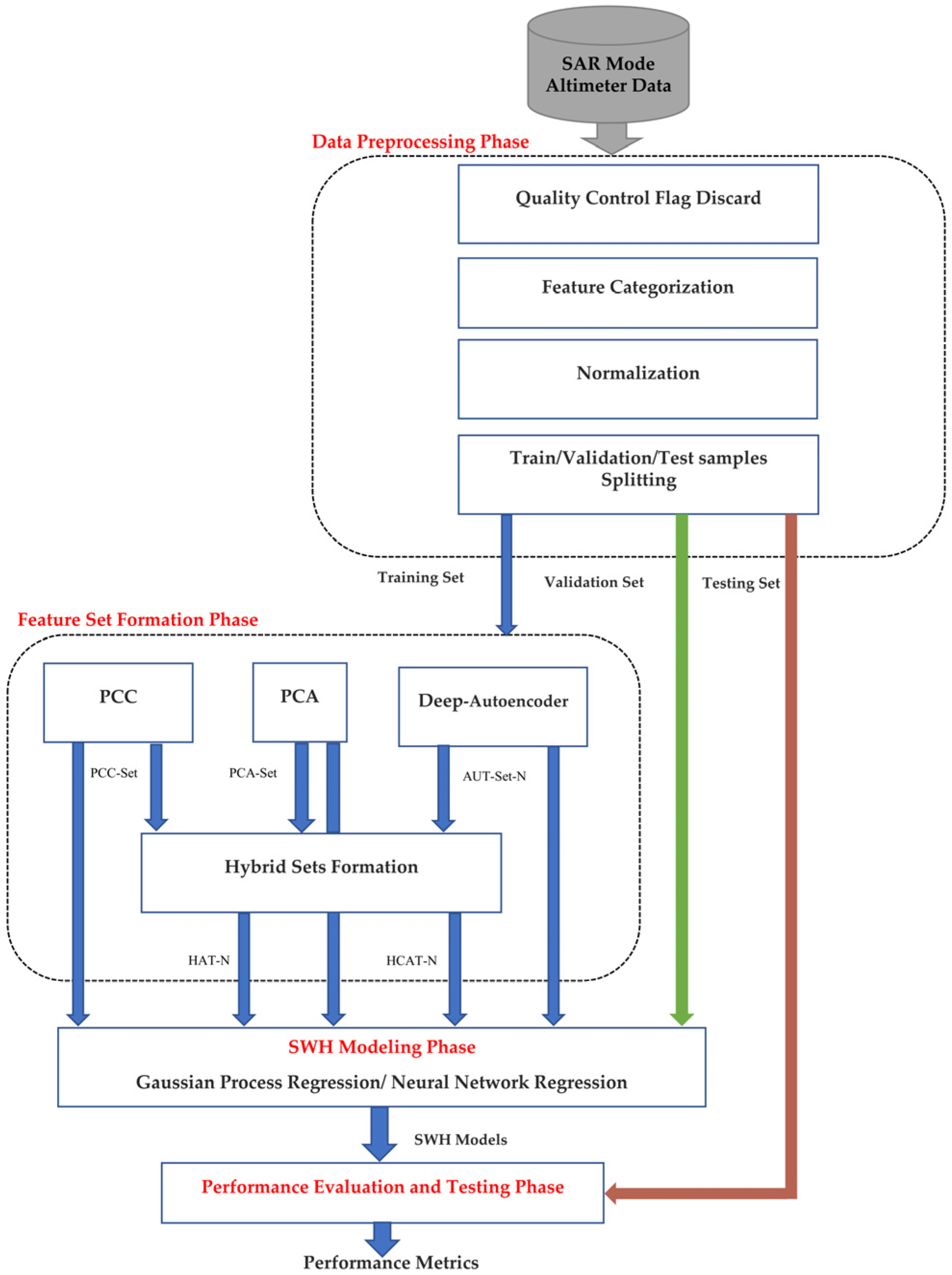
4.1. Feature Sets Formation

In this work, the calibrated SWH measured using the altimeter’s KU frequency band, SWH_KU_CAL, is considered the response variable. The KU-based features depicted in Table 4 are used to form the basic and hybrid feature sets in this experiment. The ALL-Set is composed of 16 features which represent all KU-based features except the target variable and the noncalibrated version of it. To create the PCC-Set, Pearson correlation coefficients between the input features and the target variable were calculated.

Table 5. Absolute values of Pearson correlation coefficients between SWH_KU_CAL and the KU-based features for positions P0 and P1; The features included in the PCC-Set and their correlation values are highlighted in gray.

Position P0		Position P1
Feature	|PCC|	Feature	|PCC|
SWH_KU_CAL	1	SWH_KU_CAL	1
TIME	0.0163990439235463	TIME	0.102288865532865
SWH	0.999999732870120	SWH	0.999999542438490
SIG0_KU	0.336577351930497	SIG0_KU	0.445150343609593
UWND	0.082578003464963	UWND	0.0603089207682942
VWND	0.395006371045506	VWND	0.451649290833774
WSPD_CAL	0.455941025835115	WSPD_CAL	0.579889225755999
SWH_KU_std_dev	0.173924815008291	SWH_KU_std_dev	0.371314384227738
SIG0_KU_std_dev	0.188570572892636	SIG0_KU_std_dev	0.209765508152799
DIS2COAST	0.0120031039897664	DIS2COAST	0.0702488522142944
BOT_DEPTH	0.00854422341173639	BOT_DEPTH	0.0184796601456242
WSPD	0.457591377033189	WSPD	0.579140739443493
LATSINE	0.00510651233370158	LATSINE	0.000559112294287260
LATCOSINE	0.000914880701032926	LATCOSINE	0.0223517634977151
LONGSINE	0.00209464350081526	LONGSINE	0.0108063236584730
LONGCOSINE	0.0185392818790396	LONGCOSINE	0.00620089102115493
SWH_KU_num_obs	0.0204934366118391	SWH_KU_num_obs	0.00454090475465734
SIG0_KU_num_obs	0.0204934366118391	SIG0_KU_num_obs	0.00454090475465734

depicts the absolute values of the PCC for each input feature. Normally, SWH is highly correlated with itself and its noncalibrated version. However, the recorded $\left|\mathrm{PCC}\right|$ values for the other predictors are less than 0.6. For both positions P0 and P1, the calibrated and noncalibrated wind speed based on the wind function predictors, WSPD_CAL and WSPD, record the highest correlation with the target, followed by the VWND, and then the KU-altimeter backscatter coefficient, SIG0_KU. It was noticed that the correlation between the target and the rest of the predictors is low (less than 0.1); therefore, the absolute correlation coefficients between the input features and the SWH_CAL were thresholded with a value of 0.1. Thus, the PCC-Set is formulated from the features that satisfy the criterion $\left|\mathrm{PCC}\right|\ge CCt$. The features included in the PCC-Set for P0 and P1 and their correlation values are highlighted in gray in Table 5. The SIG0_KU, VWND, WSPD_CAL, SWH_KU_std_dev, SIG0_KU_std_dev, and WSPD are included in the PCC-Set of both positions P0 and P1. However, it was noticed that for P1, the TIME variable achieved a PCC of 0.1, and therefore, it was included in the PCC-Set of this position.

As the TIME feature records different PCC values for P0 and P1, we further investigate the correlation behavior between the TIME feature and the target variable for seven geographical positions.

Table 6. Absolute values of Pearson correlation coefficients between SWH_KU_CAL and the TIME feature for seven geographical positions; # DP is the number of data points (observations).

Position	P0	P1	P2	P3	P4	P5	P6
Location	(0°N 0°E)	(0°N 0°E)	(0°N 2°E)	(0°N 3°E)	(0°N 4°E)	(0°N 5°E)	(0°N 6°E)
Period of Acquisition	26 March 2016–11 July 2018	3 March 2016–15 July 2018	7 March 2016–5 July 2018	11 March 2016–9 July 2018	1 March 2016–13 July 2018	19 March 2016–4 July 2018	9 March 2016–8 July 2018
# DP	1008	1033	1006	999	1034	1017	1089
|PCC|	0.01639	0.10228	0.06201	0.12204	0.12279	0.08812	0.02018

presents the |PCC| values for the TIME feature for the tested positions, the number of observations, and the time period over which the records were collected for each position. It is observable from Table 6 that the TIME feature generally records low correlation with the SWH. For, P1, P3, and P4, the correlation coefficient equals roughly 0.1. Therefore, for the PCC threshold used in this work, the TIME feature is included in the PCC-Set of these positions. However, the PCC values for P0, P2, P5, and P6 are 10 times lower than the other positions, and thus the TIME feature is discarded from the corresponding PCC-Set.

To generate the PCA features, the PCA algorithm was fed with the ALL-Set, and the CPV was set to 95%. The PCA-Set contains the principal components that explain 95% of the variance. It was found that for both positions P0 and P1, the PCA-Set contains the first principle component only, which captures 95% of the variance contained in the data.

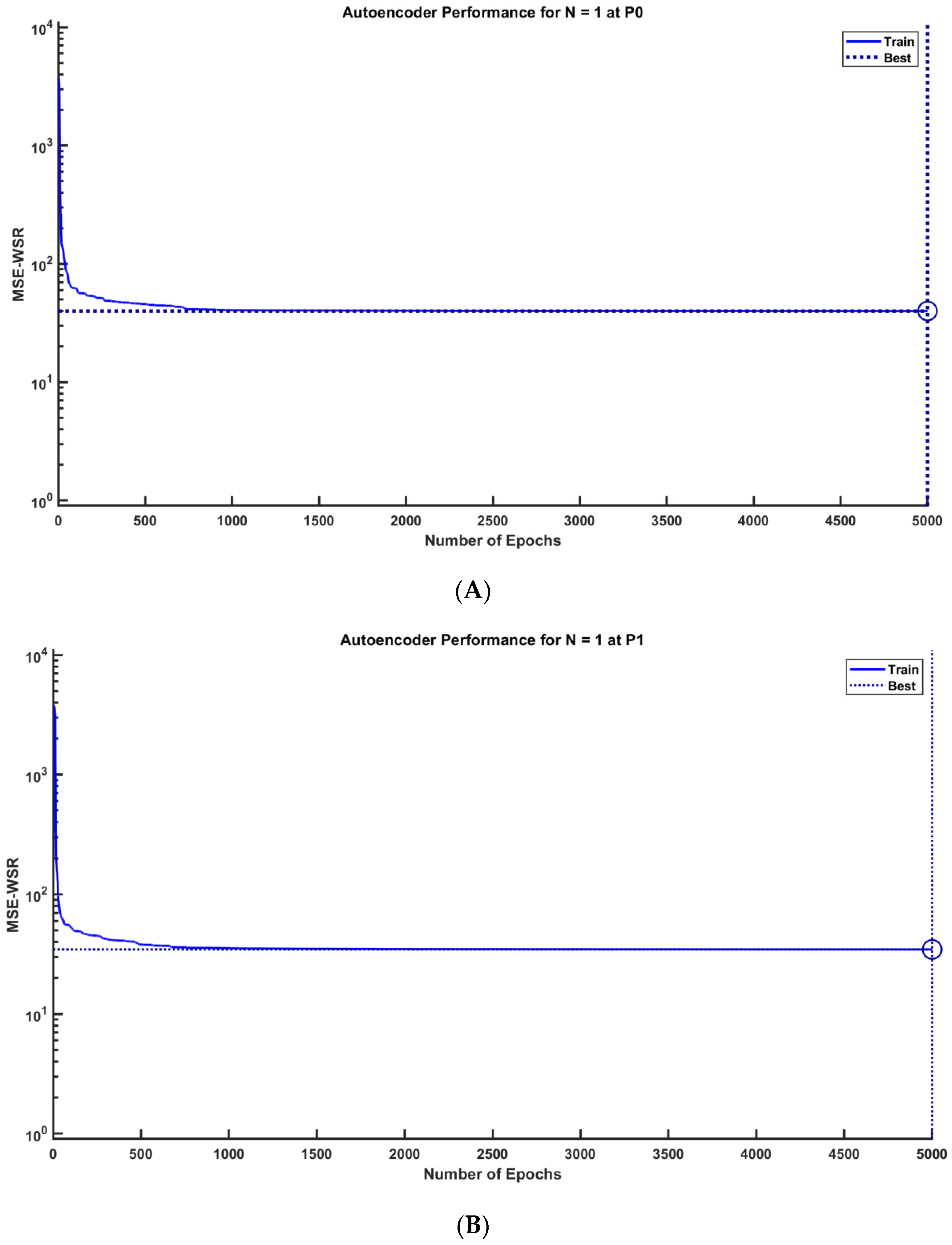
The autoencoder-derived feature sets were generated through feeding a sparse autoencoder by the ALL-Set. By setting the number of latent features output from the encoder end into a number less than the number of features in the ALL-Set, the autoencoder network was utilized as a latent-feature generator and a dimensionality reduction tool. The number of latent features output from the autoencoder, N, was set to 1, 2, and 3. Therefore, three autoencoder sets are generated: AUT-Set-1, AUT-Set-2, and AUT-Set-3. The autoencoder was trained in an unsupervised manner over 5000 epochs with the settings depicted previously in the Methods section. The performance of the autoencoder is measured using the mean squared error with weight and sparsity regularizers (MSE-WSR).

Table 7. Autoencoder performance in generating latent features from original input features for positions P0 and P1; ‘#’ denotes the number of features.

Position	# Output Features	MSE-WSR		Gradient
		Initial	Stopped	Initial	Stopped
P0	1	3.71 × 103	40	138	0.076
	2	3.71 × 103	3.22	178	0.031
	3	3.71 × 103	1.66	200	1.16
P1	1	3.79 × 103	34.7	182	0.14
	2	3.79 × 103	3.07	100	0.035
	3	3.79 × 103	2.03	246	0.079

shows the starting and stopping values of the gradient and the MSE-WSR values for positions P0 and P1 when N equals 1, 2, and 3. It is observable from

Table 8. Feature sets used for modeling SWH_KU_CAL using Positions P0 and P1 data. # F denotes the number of features included in the feature set.

Position P0			Position P1
Feature Set	# F	Included Features	Feature Set	# F	Included Features
ALL-Set	16	TIME, SIG0_KU, UWND, VWND, WSPD_CAL, SWH_KU_std_dev, SIG0_KU_std_dev, DIS2COAST, BOT_DEPTH, WSPD, LATSINE, LATCOSINE, LONGSINE, LONGCOSINE, SWH_KU_num_obs, SIG0_KU_num_obs.	ALL-Set	16	TIME, SIG0_KU, UWND, VWND, WSPD_CAL, SWH_KU_std_dev, SIG0_KU_std_dev, DIS2COAST, BOT_DEPTH, WSPD, LATSINE, LATCOSINE, LONGSINE, LONGCOSINE, SWH_KU_num_obs, SIG0_KU_num_obs.
PCC-Set	6	SIG0_KU, VWND, WSPD_CAL, SWH_KU_std_dev, SIG0_KU_std_dev	PCC-Set	7	TIME, SIG0_KU, VWND, WSPD_CAL, SWH_KU_std_dev, SIG0_KU_std_dev.
PCA-Set	1	First principal component explaining 95% of data variance.	PCA-Set	1	First principal component explaining 95% of data variance.
AUT-Set-1	1	Single latent feature output from the encoder	AUT-Set-1	1	Single latent feature output from the encoder
AUT-Set-2	2	Two latent features output from the encoder	AUT-Set-2	2	Two latent features output from the encoder
AUT-Set-3	3	Three latent features output from the encoder	AUT-Set-3	3	Three latent features output from the encoder
HCAT-1	8	Hybrid set composed by fusing the features in PCC-Set, PCA-Set, and AUT-Set-1	HCAT-1	9	Hybrid set composed by fusing the features in PCC-Set, PCA-Set, and AUT-Set-1
HCAT-2	9	Hybrid set composed by fusing the features in PCC-Set, PCA-Set, and AUT-Set-2	HCAT-2	10	Hybrid set composed by fusing the features in PCC-Set, PCA-Set, and AUT-Set-2
HCAT-3	10	Hybrid set composed by fusing the features in PCC-Set, PCA-Set, and AUT-Set-3	HCAT-3	11	Hybrid set composed by fusing the features in PCC-Set, PCA-Set, and AUT-Set-3
HAT-1	2	Hybrid set composed by fusing the features in PCA-Set and AUT-Set-1	HAT-1	2	Hybrid set composed by fusing the features in PCA-Set and AUT-Set-1
HAT-2	3	Hybrid set composed by fusing the features in PCA-Set and AUT-Set-2	HAT-2	3	Hybrid set composed by fusing the features in PCA-Set and AUT-Set-2
HAT-3	4	Hybrid set composed by fusing the features in PCA-Set and AUT-Set-3	HAT-3	4	Hybrid set composed by fusing the features in PCA-Set and AUT-Set-3

that the MSE-WSR decreases with increasing the number of output features. Increasing the number of output features helps including more details from the original data, which aids in reducing the output cost. However, increasing the number of latent features would not guarantee better prediction performance of the regression model. Therefore, the maximum number of output features from the encoder was selected to be 3. This setting helped reduce the computational load and time, and it was proved by experiment to be sufficient to enhance the regression model performance. It is also noticed that the values of the gradient and MSE are the highest at the beginning of the training process and the lowest at the stopping, which is a normal result of algorithm learning. The behavior of the autoencoder performance against the training epochs is depicted in Figure 5, which shows sample plots of the autoencoder performance in Experiment 1 for N = 1 at P0 and P1.

Hybrid feature sets were formed by merging features from the basic feature sets. Table 8 depicts the features in the basic and hybrid feature sets and their number of features used for SWH_KU_CAL modeling for Positions P0 and P1.

The performance of the GPR and NNR models trained individually by the basic and hybrid sets for modeling SWH_KU_CAL is depicted in

Table 9. SWH_KU_CAL prediction performance of GPR and NNR models trained on KU-based feature combination sets for Position P0; Best models are highlighted in dark gray, and the second-best performance regressor is highlighted in light gray; ‘#’ denotes the number of features.

Position: P0		GPR			NNR
Feature Set	# F	RMSE	R2	Kernel Function	RMSE	R2
ALL-Set	16	0.29262	0.41	Rational Quadratic	0.31634	0.32
PCA-Set	1	0.12792	0.87	Rational Quadratic	0.29677	0.31
PCC-Set	6	0.31881	0.36	Matern 5/2	0.33156	0.31
AUT-Set-1	1	0.20963	0.73	Squared Exponential	0.31853	0.37
HAT-1	2	0.12188	0.91	Squared Exponential	0.33354	0.36
HCAT-1	8	0.29877	0.38	Rational Quadratic	0.2625	0.52
AUT-Set-2	2	0.12985	0.9	Rational Quadratic	0.24259	0.64
HAT-2	3	0.11724	0.92	Rational Quadratic	0.2601	0.6
HCAT-2	9	0.32058	0.32	Rational Quadratic	0.29551	0.4
AUT-Set-3	3	0.14791	0.89	Squared Exponential	0.31347	0.49
HAT-3	4	0.13112	0.8	Rational Quadratic	0.27078	0.13
HCAT-3	10	0.39404	0.23	Squared Exponential	0.33302	0.45

and

Table 10. SWH_KU_CAL prediction performance using GPR and NNR trained by various feature combinations for Position P1; ‘#’ denotes the number of features.

Position: P1		GPR			NNR
Feature Set	# F	RMSE	R2	Kernel Function	RMSE	R2
ALL-Set	16	0.25525	0.44	Exponential	0.27248	0.36
PCA-Set	1	0.11961	0.86	Rational Quadratic	0.22502	0.49
PCC-Set	7	0.24238	0.4	Rational Quadratic	0.24024	0.41
AUT-Set-1	1	0.17635	0.64	Rational Quadratic	0.2258	0.33
HAT-1	2	0.10414	0.89	Squared Exponential	0.20098	0.6
HCAT-1	9	0.23234	0.47	Exponential	0.22728	0.49
AUT-Set-2	2	0.1046	0.87	Exponential	0.19511	0.54
HAT-2	3	0.1113	0.85	Matern 5/2	0.1889	0.58
HCAT-2	10	0.23529	0.31	Exponential	0.2236	0.38
AUT-Set-3	3	o.12272	0.84	Exponential	0.18277	0.65
HAT-3	4	0.13351	0.82	Matern 5/2	0.19522	0.61
HCAT-3	11	0.2367	0.37	Exponential	0.22549	0.41

. Table 9 shows the RMSE and R2 values for the regressors trained on position P0 data, while Table 10 presents the regression performance for position P1. For position P0, the results show that GPR models recorded higher prediction performance than the NNR models for all feature sets. It was noticed that the basic feature sets generally yielded lower regression performance than the hybrid sets. It is noticeable that GPR models trained by the HAT sets recorded higher performance than the other hybrid sets. The best GPR model records the highest R2 value of 0.92 and an RMSE value of 0.11724. This model has a Rational Quadratic kernel and was trained by the HAT-2 set. The second-best GPR model recorded an R2 value of 0.91 and was trained by the hybrid set HAT-1. On the other hand, the NNR model trained on the AUT-Set-2 set recorded the highest performance, followed by the HAT-2-based model over the other NNR models. The best models are highlighted in dark gray, and the second-best performance regressor is highlighted in light gray in Table 9 and Table 10.

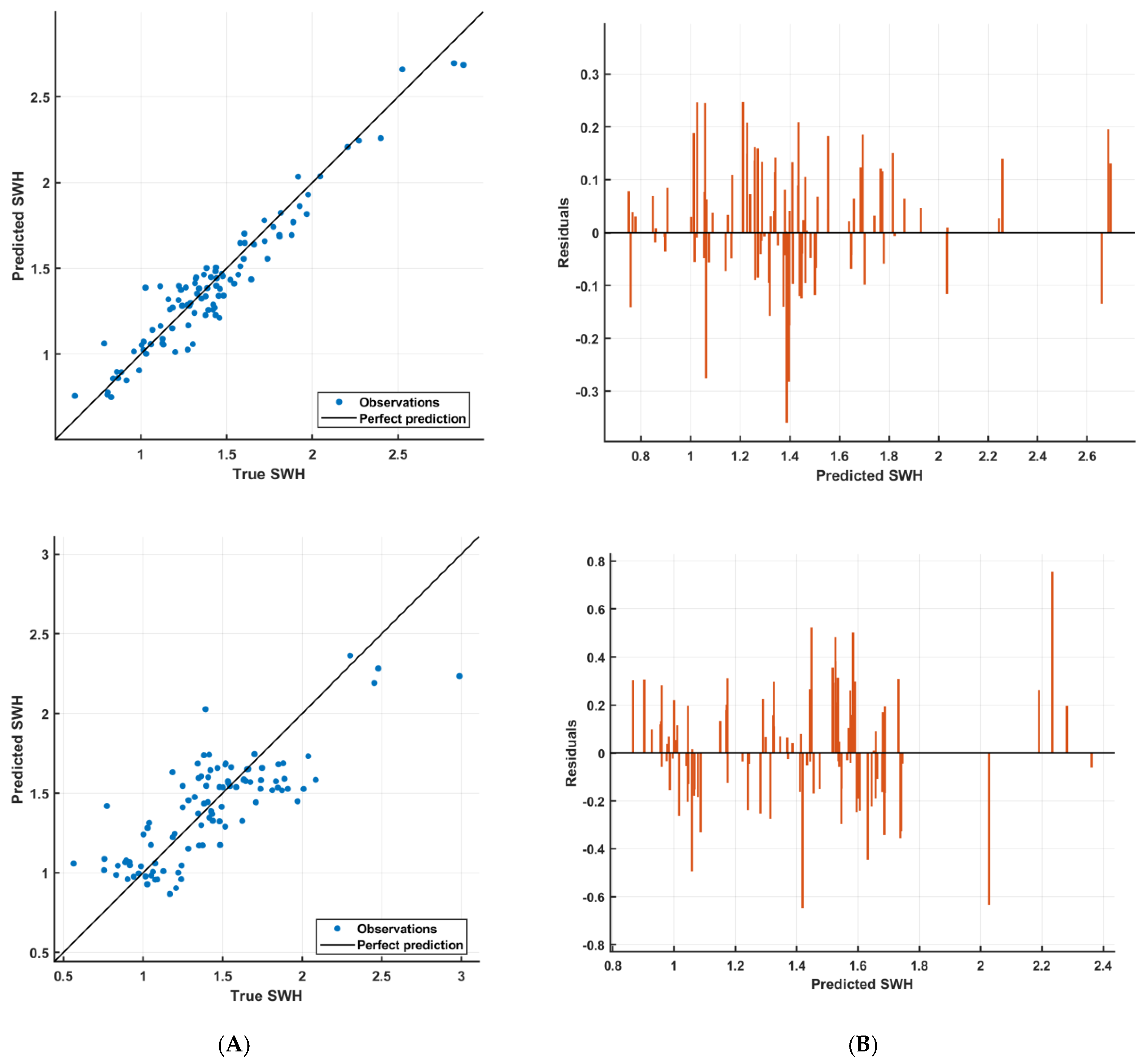
Figure 6 illustrates the goodness of fit of the SWH predictions generated for the test set by the best GPR and NNR models trained on P0 data. The plots of Figure 6 show the predicted versus true values of the response, SWH_KU_CAL, and the residuals for the best GPR and NNR models highlighted in dark gray in Table 9. It is clear that the GPR model predictions are closer to the diagonal line, which represents the perfect prediction, than those predicted by the NNR. This observation is consistent with the high R2 value of the GPR model and is confirmed by the residual plot. The residuals of the GPR predictions range between [−0.3, 0.3], while it ranges from [−0.8 to 0.7] for the NNR predictions.

For position P1, it is clear from Table 9 that the GPR model trained on the HAT-1 set achieved the highest performance compared with the NNR based on the highest R2. The second-best performance is recorded by the AUT-Set-2-based GPR model with an exponential kernel. On the other hand, the best NNR model recorded 0.65 for the coefficient of determination and was trained by the AUT-Set-3. The second-best performer was the HAT-3-based NNR model. Similarly to P0, the GPR models achieved higher performance that the NNR. It is observed that the regressors trained on the PCC-Set, and the hybrid features based on it, the HCAT sets, suffered from poor performance. This could be interpreted as a result of the low correlation between the predictors in the PCC-Set and the target, which hindered the improvement of the model performance, even after fusing the PCC, PCA, and AUT features together. It was also noticed that the HAT sets provides better regression performance than the PCA-Set and the AUT sets. This indicates the improving impact of the autoencoder features on the prediction performance when added to the PCA features.

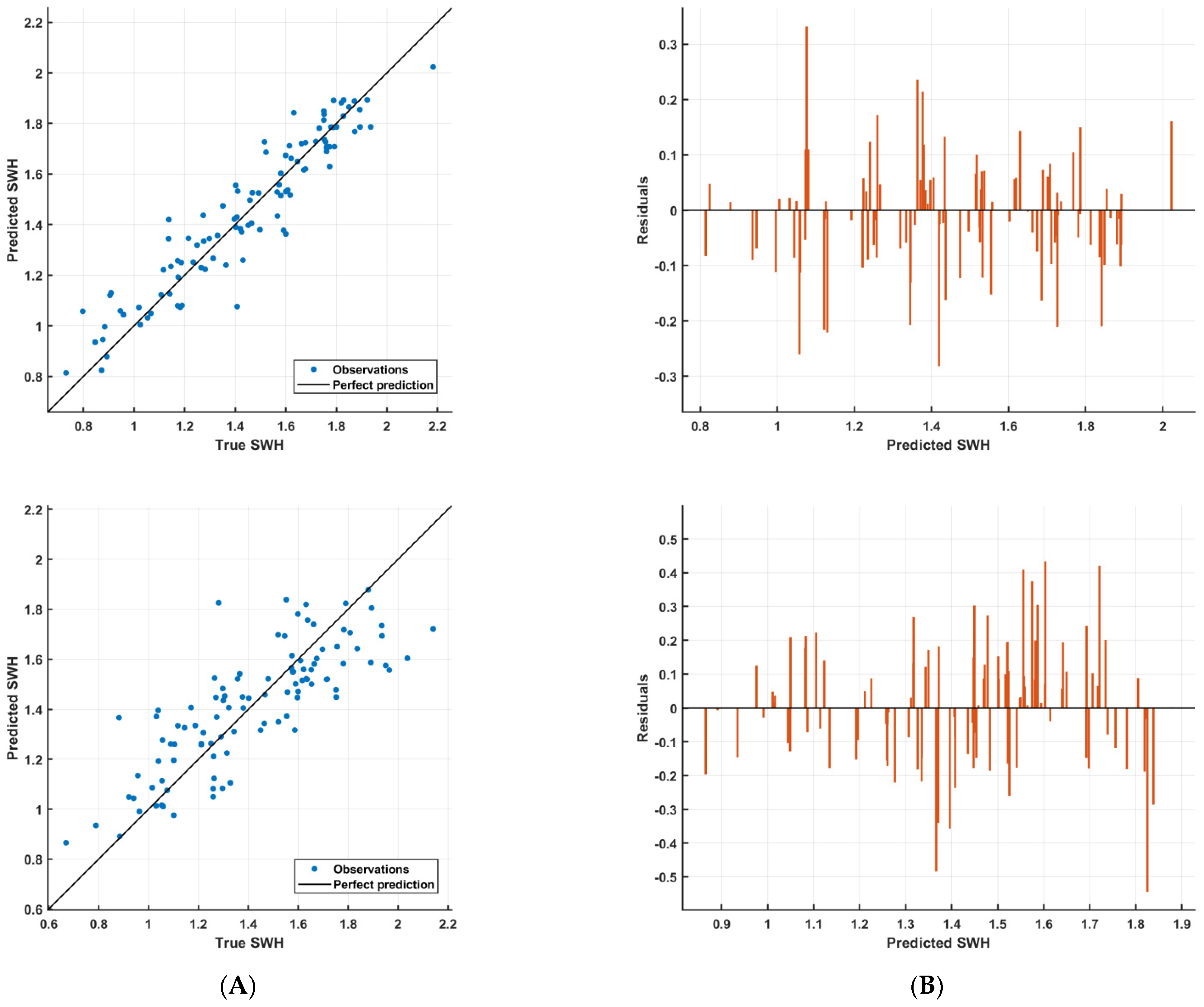
Figure 7 presents the goodness of fit of the SWH predictions generated by the best GPR and NNR models trained on P1 data. The plots of Figure 7 illustrate the predicted versus true values of the response, SWH_KU_CAL, and the residuals for the best GPR and NNR models on the test set. It is clear that the predictions are scattered roughly symmetrically around the diagonal line for both GPR and NNR. The predictions of the GPR model are closer to the diagonal line than the NNR predictions. This observation is reflected in the residual plots, which show the difference between the true and predicted target. The error in the predictions with respect to the SWH true values ranges between [−0.3, 0.4] for the GPR model and [−0.6, 0.5] for the NNR model. The performance plots of Figure 5 reveal the superiority of the GPR model over the NNR.

To summarize the findings of the current research, the prediction performance of the first and second-best regressors recorded by the GPR and NNR models for position P0 and P1 is presented in

Table 11. Summary of the performance of best SWH regression models for position P0 and P1; ‘#’ denotes the number of features.

Position	Rank	GPR				NNR
		Features Set	# F	RMSE	R2	Feature Set	# F	RMSE	R2
P0	1	HAT-2	3	0.11724	0.92	AUT-Set-2	2	0.24259	0.64
	2	HAT-1	2	0.12188	0.91	HAT-2	3	0.2601	0.6
P1	1	HAT-1	2	0.10414	0.89	AUT-Set-3	3	0.18277	0.65
	2	AUT-Set-2	2	0.1046	0.87	HAT-3	4	0.19522	0.61

. The highest average RMSEs obtained over the two positions are 0.11069 and 0.21268 for the GPR and NNR models, respectively. It was noticed that The GPR models provides better prediction performance than the NNR models in terms of RMSE and R² metrics for both positions. This observation was further proved by the residual plots of the regression models. It was noticed that the HAT feature sets boosted the GPR model performance over that trained by the basic PCA or AUT feature sets individually. In contrast, pure autoencoder features yielded better performance of the NNR models over that of NNR models trained individually by the basic as well as the hybrid sets. Moreover, it was observed that the HCAT sets yielded lower prediction performance than the AUT sets and HAT sets for both the GPR and NNR. This observation could be referred to the low correlation of the original predictors in the PCC-Set with the response variable. Adding such features to the PCA and autoencoder-derived features hindered the significant improvement of the model performance. It was shown that the autoencoder-derived features aid in providing improved prediction performance of the GPR and NNR models over the basic feature sets.

To discuss the results from the sea area (site) perspective, the PCC analysis showed that the DIST2COAST, BOT_DEPTH, LONGITUDE, and LATITUDE-related features are not significant with respect to SWH from the correlation perspective for both positions P0 and P1 (these features recorded very low PCC values). The observation that could be made here is that these site-related features do not contribute significantly to SWH measurements. However, the measured features showed generally higher PCC values than the site-related features, and thus could effectively affect to SWH measurements. The measured features, especially the wind speed, are characterized by their intermittent and stochastic nature. Moreover, the data of the two used positions were collected over different times, and the two positions are approximately 69 miles apart to the east, which means that the two sites had different sea states at the time of data acquisition. Such variations would interpret the difference in the best feature sets of the two positions (HAT-2 for P0 versus HAT-1 for P1 for the GPR and AUT_Set-2 versus AUT-Set-3 for the NNR). Nonetheless, the best feature sets for both sites were based on the autoencoder-derived features, which reveal the effectiveness of this technique in extracting significant features from the original data features. The autoencoder-derived features even improved the prediction performance when combined with the PCA features (in the HAT feature set).

4.2. Hypothesis Testing for Feature Significance

In order to reinforce the findings of the current study, the significance of the features included in the feature sets that yielded the highest prediction performance of the GPR and NNR is examined using hypothesis testing. In the present study, the ANOVA F-statistics test was utilized to identify the significance of the features included in the HAT-2 and AUT-Set-2 feature sets of P0 data as well as the features of HAT-1 and AUT-Set-3 features of P1. In this test, the input features are used to model the response variable using a linear regression model and determine the significance of the predicted model coefficients through statistical metrics, namely the F-value and p-value. The null hypothesis of the test, H0, assumes that there is no relationship between the response variable, SWH, and the input features i.e., all dependent variable coefficients are zero. On the other hand, the alternative hypothesis, H1, implies that the model is accurate if there is at least one instance where any of the dependent variable coefficients are nonzero. The outcomes of the ANOVA Test of the significance of the aforementioned four feature sets in predicting the SWH are depicted in

Table 12. Outcomes of ANOVA Test of Autoencoder-based features’ significance in predicting the SWH using P0 and P1 data.

Position	Feature Set	Feature Symbol	Test F-Value	Test p-Value
P0	HAT-2	F1	27.9	8.19 × 10−7
		F2	30.70119	4.08 × 10−8
		F3	49.92715	3.46 × 10−12
	AUT-Set-2	F1	11.57716	0.0007
		F2	43.37607	8.15 × 10−11
P1	HAT-1	F1	7.9	0.004
		F2	7.3	0.006
	AUT-Set-3	F1	464.4652	4.75 × 10−82
		F2	17.44876	3.27 × 10−5
		F3	23.47258	1.5 × 10−6

. The significance level is considered 0.05 for the p-value. The values obtained for both the F-value and the p-value indicate that there is a significant association between the response variable, SWH, and the input predictors for all feature sets. Therefore, the Null hypothesis can be rejected, and the significance of the examined autoencoder-derived features and hybrid features is confirmed.

The prediction performance of the SWH regression model trained on the feature sets generated using the proposed deep-learning-based approach is further evaluated against the state of the art. Numerous research studies have addressed the problem of SWH prediction from satellite data from different perspectives and using various types of satellite data. In order to have a meaningful benchmarking, only studies that tackled the problem of SWH prediction using the IMOS Surface Waves Sub-Facility dataset are considered for comparison. The IMOS Surface Waves Sub-Facility dataset is a recent dataset that was published in 2019 and has received slight coverage in the literature. Only a single recent study was found to use the IMOS dataset for the prediction of SWH. The study by Quach et al. [35] investigated the use of deep learning to predict significant wave height from a dataset created from collocations between the Sentinel-1SAR and altimeter satellites’ observations from the IMOS dataset. Quach et al. integrated features from the IMOS altimeter data with a number of CWAVE features that were derived from the SAR image modulation spectra and developed a deep-learning-based regression model for SWH prediction. The results of that study show an improved RMSE of the deep learning model of 0.26. In our study, we employed the autoencoder deep learning network to generate significant features from the altimeter observations for the prediction of SWH using GPR and NNR. The proposed deep-learning-based feature generation method yielded average RMSE values of 0.11069 and 0.21268 for the GPR and NNR models, respectively. Therefore, the deep-learning-based SWH modeling approach proposed in the present study provides improved prediction performance over the state of the art.

5. Conclusions

In this research, we introduced a framework to extract features from SAR mode altimeter data using a hybrid deep-learning-based approach for the prediction of SWH. The proposed approach is based on the proficiency of the autoencoder neural network in representing input features in the latent space. The proposed framework is composed of four phases: data preprocessing, feature sets formation, SWR modeling, and model evaluation and testing. After the data were preprocessed, a number of basic feature sets were created from the input data. The basic sets include the ALL-Set, PCC-Set, PCA-Set, and AUT-Set-N. Multiple hybrid feature sets were further formed using various combinations of the PCC, PCA, and AUT feature sets, as well as the HAT, and HCAT sets. These sets were used for modeling SWH using the GPR and NNR. The regression models were validated using a 5-cross validation scheme and tested on a holdout test set. The prediction performance of the SWH models trained on the hybrid feature sets are compared with that trained by the basic PCC, PCA, and autoencoder-driven feature sets as well as all input features set. The results show that hybridizing the PCA and AUT feature sets yielded improved prediction performance for the GPR models, while pure autoencoder-derived features boasted the performance of the NNR models. The significance of the autoencoder-based pure and hybrid feature sets was proven through hypothesis testing. The presented results reveal the significance of the autoencoder-derived features in improving the performance of SWH prediction from altimeter data. In general, the findings of this study reveal the superiority of the autoencoder deep learning network in generating latent features that aid in improving SWH prediction performance over traditional feature extraction methods.