Abstract
Sea fog detection has received widespread attention because it plays a vital role in maritime activities. Due to the lack of sea observation data, meteorological satellites with high temporal and spatial resolution have become an essential means of sea fog detection. However, the performance is unsatisfactory because low clouds and sea fog are hard to distinguish on satellite images because they have similar spectral radiance characteristics. To address this difficulty, a new method based on a two-stage deep learning strategy was proposed to detect daytime sea fog in the Yellow Sea and Bohai Sea. We first utilized a fully connected network to separate the clear sky from sea fog and clouds. Then, a convolutional neural network was used to extract the differences between low clouds and sea fog on 16 Advanced Himawari Imager (AHI) observation bands. In addition, we built a Yellow and Bohai Sea Fog (YBSF) dataset by pixel-wise labelling AHI images into three categories (i.e., clear sky, cloud, and sea fog). Five comparable methods were used on the YBSF dataset to appraise the performance of our method. The vertical feature mask (VFM) generated by Cloud-Aerosol Lidar with Orthogonal Polarization (CALIOP) was also used to verify the detection accuracy. The experimental results demonstrate the effectiveness of the proposed method for sea fog detection.
1. Introduction
Compared with daytime fog detection over land, fewer observation stations are mounted at sea, therefore, it is a challenge to detect the sea fog with sparse observation data for further investigation. In recent decades, researchers have leveraged meteorological satellite data with high temporal and spatial resolution for large-scale sea fog detection [1]. The current mainstream strategy for sea fog detection is selecting the optimum threshold values based on the radiation property of sea fog. Hunt [2] theoretically proved that the specific emissivity of opaque water clouds such as fog and low clouds in the short-wave infrared bands was significantly lower than that in the long-wave infrared bands. Based on this assumption, Eyre et al. [3] adopted the brightness temperature difference (BTD) between the 3.7 μm and 11 μm bands of the NOAA polar-orbiting satellite to detect heavy fog at night. Ellrod [4] successfully applied the BTD method to the GOES geostationary satellite for long-term fog monitoring and analysis. Because the short-wave infrared channel received both the radiation of the target itself and the reflection of the solar radiation from the target during the daytime, the BTD method cannot be directly applied for daytime fog detection. Nevertheless, as more visible bands are available during the daytime, Bendix, et al. [5] utilized visible and near-infrared band data to conduct daytime fog detection with Moderate Resolution Imaging Spectroradiometer (MODIS) data.
In order to make full use of the multi-spectral satellite data, the spectral radiance characteristic difference of fog and other targets was analyzed and compared based on a large number of satellite observations [6,7]. Hao et al. [8] simulated the radiation properties of fog/clouds with the streamer radiative transfer model under different fog/cloud microphysical and observational conditions. The spectral radiance characteristics provide a reliable basis for the band selection of sea fog detection. Zhang et al. [9] discussed a variety of spectral indices designed for sea fog remote sensing detection including the normalized difference of snow index (NDSI) [10] and the normalized difference near-infrared water vapor index (NWVI) [11], and built a multi-source satellite-based full-time sea fog detection model.
Considering that the remote sensing data are easily affected by factors such as instrument difference, solar elevation angle variations, and seasonal changes, it is not suitable to adopt the same threshold values to carry on sea fog detection from the data observed by satellites in different regions and at different times. Cermak and Bendix [12] dynamically selected the threshold based on the histogram of radiance difference in a local area, which could overcome the above challenges to a certain extent. Drönner et al. [13] first divided the European area covered by the MSG satellite into uniform grids, then dynamically determined the low cloud and heavy fog separation threshold in each grid according to the histogram of the BTD, and used OpenCL parallel processing to monitor fog continuously. Kim et al. [14] proposed a decision tree (DT) approach for sea fog detection based on Geostationary Ocean Color Imager (GOCI) observations in combination with Advanced Himawari Imager (AHI) data onboard the Himawari-8 satellite, and reduced the sensitivity to the highly variable environment.
Although the dynamic threshold methods improve the accuracy of sea fog detection, it is difficult to determine the optimum threshold value based on the peaks and troughs of the spectral histogram, since it varies considerably. With the development of deep learning, convolutional neural networks (CNN) have widely been used in many fields such as image recognition [15] and target detection [16,17] and provide state-of-the-art performance. CNNs can learn discriminative texture features by a training dataset. In contrast, it is inefficient for traditional approaches to define and extract features of sea fog due to the complexity of natural texture and patterns. However, deep learning methods are rarely used in the research of sea fog detection because it has a high cost in terms of human resources for labeling the training datasets [18]. Only a few articles have described the application of deep learning in sea fog detection. Si et al. [19] extracted 33-dimensional combined features from the AHI data including the reflectance/brightness temperature of each band of the AHI data and the texture features extracted from the 0.64 μm band, and utilized a fully connected neural network for daytime sea fog recognition, achieving an accuracy of 82.63%. Jeon et al. [20] generated 120 images of each category with a size of 100 × 100 pixels from GOCI and used them to fine tune the pre-trained VGG19 [21] and ResNet50 [22]. Although the highest accuracy in the experiment reached 91.6%, the model seemed to lack sufficient robustness due to the small amount of training data for the image classification task. Zhou et al. [23] proposed a new sea fog detection dataset (SFDD) that labeled 1032 sea fog images recorded by the GOCI over the Yellow Sea and Bohai Sea, and designed a dual-branch sea fog detection network (DB-SFNet) to jointly extract discriminative features from both the visual and statistical domains.
To this end, in this paper, we constructed a daytime sea fog remote sensing dataset called YBSF (Yellow and Bohai Sea Fog). Compared with the GOCI data (eight channels, 0.41 μm~0.68 μm), the YBSF dataset based on Himawari-8 (16 channels, 0.47 μm~13.3 μm) can provide more spectral information for sea fog detection, and the YBSF dataset was also available for peer researchers. Two meteorological experts labeled and cross-validated the dataset, which classified each pixel in 24 AHI images into four categories: clear sky, land, cloud, and sea fog, which were assigned as the ground truth. Based on this dataset, a two-stage neural network was proposed for daytime sea fog detection. Unlike other sea fog detection methods based on machine learning that distinguish clear sky, cloud, and sea fog at the same time, or treat clear sky and cloud as the same category, the proposed method first regarded sea fog and cloud with similar spectral characteristics as one category and designed a multilayer perceptron (MLP) to distinguish clear sky and non-clear sky pixels. Then, the proposed CNN model was used to extract more discriminative spectral and texture features to separate sea fog from cloud. The proposed method was trained and tested based on the YBSF dataset, and was also validated using the vertical feature mask (VFM) generated by Cloud-Aerosol Lidar with Orthogonal Polarization (CALIOP) onboard the Cloud-Aerosol Lidar and Infrared Pathfinder Satellite Observation (CALIPSO) [1]. Experimental results on the YBSF dataset showed that the rich spectral and textural features extracted by the proposed neural network were more capable of separating cloud and fog than the comparative methods.
2. Data
2.1. Study Areas
In this paper, we selected the northern part of the Yellow Sea and Bohai Sea as the study area. Figure 1 shows a sea fog occurrence in that area on 18 March 2020, at 01:00 UTC. The Yellow–Bohai Sea area has experienced heavy fog events over a considerable fraction of the year [24]. Sea fog in this area is mostly from advection fog events, which are generated when the prevailing south wind brings warm and humid air to the cold northern waters during the sea fog season from March to August [25,26,27].
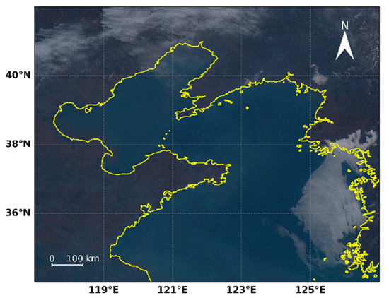
Figure 1.
Himawari-8 true color image (composited by AHI observation bands B01, B02, and B03) captured on 18 March 2020, at 01:00 UTC. This area includes the Bohai Sea and the northern part of the Yellow Sea, with latitude and longitude ranging from 34°N to 42°N, 117°E to 127°E, respectively. The solid yellow lines represent coastlines.
2.2. YBSF Dataset
Himawari-8 is the latest generation of the geostationary meteorological satellite funded by the Japan Meteorological Agency and developed by Mitsubishi Electric Corporation, which is equipped with the most advanced optical sensor AHI. The AHI consists of 16 observation bands covering visible, near-infrared, and infrared bands, with spatial resolution varying between 0.5 km and 2 km, and offers full disk observation data every 10 min. Table 1 shows the details of the 16 AHI bands along with the related wavelengths [28].

Table 1.
The Himawari-8/AHI specifications.
In this paper, we collected 24 sea fog events captured in 2020 from the study area to construct the YBSF dataset. Each pixel of the dataset was labeled as one of four categories, namely, ground, clear sky (i.e., the sea water pixels, which is not covered by cloud or fog), sea fog, and clouds, respectively, by two experienced meteorological experts, based on the spectral differences between different categories, and the manually labeled results were taken as the ground truth. Since the radius of fog droplets is close to the wavelength of the near-infrared channel, according to the Mie scattering theory, the reflectivity of this channel is greater than that of the visible channel, while the reflectivity of cloud droplets in the visible channel is greater than that in the near-infrared channel. Meanwhile, as the sea fog is close to the ground, its brightness temperature in the infrared channel is higher than that of the cloud. The 500 m spatial resolution of 0.64 μm data also provides rich texture information for cloud and sea fog discrimination. Thus, we synthesized color images with 0.64 μm, 1.6 μm, and 11.2 μm band data to help experts label the dataset more accurately.
For the proposed method, 80% of the YBSF dataset was used for training and the rest was used for testing. We randomly sampled 10,000 clear sky pixels and 10,000 non-clear sky pixels from the training set for the first-stage MLP model training. For the second-stage CNN model, we randomly sampled 50,000 cloud-centered image patches and sea fog-centered image patches, respectively. The training samples of the extraction procedure is illustrated in Figure 2. The selection of the image patch size will be discussed in Section 4.
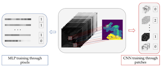
Figure 2.
The extraction procedure of the samples and corresponding labels for the MLP and CNN model. The sea fog, clear sky, cloud pixels are indicated in green, blue and yellow, respectively in the middle of the panel.
3. Method
Detecting sea fog from satellite images remains challenging for traditional methods based on thresholds because remote sensing spectral data vary over time and space. Neural networks can extract high-level feature representation (i.e., texture) and are naturally considered to be a reasonable choice to address the difficulty of sea fog detection. Thus, we propose a new sea fog detection method using a two-stage neural network architecture, which integrates multi-spectral and spatial information of the AHI data. The first stage was dedicated to recognizing clear sky, and the second stage was committed to distinguishing between clouds and sea fog areas. Benefitting from the step-by-step method, we located the sea fog region with high accuracy. In this section, we initially sketched the components of the proposed neural network architecture and then elaborated on the details of each procedure. The overall flow chart of the proposed method is illustrated in Figure 3. Each 16-dimensional spectral pixel of the AHI image was first input to a fully connected MLP for clear sky pixel detection. Then, for each non-clear sky pixel, an image patch was extracted centered on this pixel as the input of the convolutional neural network to fully extract the spatial information for cloud and sea fog separation.
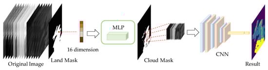
Figure 3.
Flow chart of the proposed two-stage fog detection algorithm. Overall, it contained a fully connected MLP and a convolutional neural network. The sea fog, clear sky, cloud pixels are indicated in green, blue and yellow, respectively in the result.
3.1. Pre-Processing
The satellite images need to be preprocessed into a suitable format before being fed to the neural network. Each original AHI data of the survey area were converted into a 16-band image with geographic latitude/longitude projection. The spatial resolution of each image was 0.005 degrees (~0.5 km), thus the size of the image was 2000 × 1600. After that, the land mask was applied to each image to obtain the region of interest (ROI), as shown in Figure 3. All pixels in the ROI were classified into three categories: clear sky, sea fog, or clouds, and the pixels of the land were excluded.
3.2. Distinguish Clear Sky from Clouds and Sea Fog
It is widely accepted that the spectral properties of the clear sky and sea water are very different from those of clouds. To obtain as much spectral information as possible, we employed a MLP architecture that took 16-band AHI pixels as the input and predicted whether the pixels were clear sky or not. The MLP consisted of two hidden layers with ReLU (rectified linear unit) as the activation function, as shown in Figure 4. The first hidden layer was fully connected to the original 16-dimensional spectral vector to extract the 4-dimensional combined spectral feature vector. Through the second hidden layer, the spectral features were continuously fused and reconstructed to obtain 3-dimensional deep spectral features. The output layer comprised two perceptions, which classifies the input pixel into two categories (i.e., clear sky and non-clear sky). After excluding the clear sky areas through MLP, the non-clear sky pixels of the ROI (consisting of both cloud area and sea fog area) will serve as input to the second stage to distinguish sea fog from clouds.
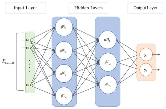
Figure 4.
The architecture of the proposed MLP for clear sky detection.
3.3. Distinguish Sea Fog from Clouds
Sea fog can be regarded as a special kind of cloud, which has certain similarities with clouds in spectral characteristics. Therefore, it is difficult to distinguish clouds and sea fog by spectral vector directly. The large-scale observation capability of satellite cloud images can obtain the spatial characteristics, which is an effective criterion to separate sea fog from clouds. To fully exploit the differences in texture and spatial structure of these two categories in the satellite images, we adopted a CNN-based architecture for sea fog detection, as shown in Figure 5. For each non-clear sky pixel, a 65 × 65 sized image patch with 16 bands centered at the pixel was cropped as the model input. The spectral and spatial features of the image patch were extracted at different scales through three convolutional layers, each followed by a max-pooling layer. The feature map was then flattened and fed into two fully connected layers to classify the center pixel of the image patch as sea fog or clouds. When training the model, random flip and rotation were also adopted for data augmentation.
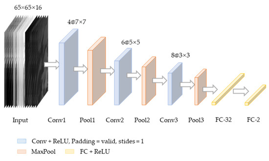
Figure 5.
The architecture of the CNN proposed in this paper. The architecture consisted of three convolutions with a stride of 1, followed by a ReLU nonlinearity. Each convolution was separated by a 2 × 2 max pooling layer. Two regular densely connected layers were pushed into the stack of the structure to reduce the dimensions to two (sea fog and clouds). ReLU activations were also applied to these two fully connected layers.
4. Experimental Results and Analysis
In this section, the prediction performance of the proposed two-stage neural network is reported on the YBSF dataset. We conducted the experiments with the proposed algorithm and other state-of-the-art sea fog detection methods. We compared different methods with five evaluation metrics including false alarm ratio (FAR), probability of detection (POD), critical success index (CSI), percentage error (ERR), and Hanssen–Kuiper skill score (KSS). Definitions of the metrics are as follows:
where FP, FN, TP, and TN indicate false positives, false negatives, true positives, and true negatives.
Furthermore, to validate the effectiveness of the proposed method, we applied the CALIPSO VFM data to evaluate the sea fog detection accuracy, which will be discussed in Section 4.3.
4.1. Image Patch Size Analysis
In this section, the size of the image patch was investigated to assess its impact on the sea fog detection accuracy. The detection results with different image patch sizes showed that the sea fog detection accuracy was relatively high when the patch size was 65 × 65, as elaborated in Table 2, the best value for each evaluation matric is in bold. The reason is that an appropriate image patch can capture more abundant texture information of the sea fog and thus enhance the discrimination level of the CNN for the central pixel of the image patch. However, when the image patch is too large, it might include objects with different categories, which causes confusion in the recognition of the central pixel.
Table 2.
Classification accuracy of the proposed method with different image patch sizes.
4.2. Comparison with Other Methods
To validate the superior recognition performance of the proposed algorithm, in this section, we compare the results with five state-of-the-art sea fog detection methods including support vector machine (SVM), MLP, VGG16 [14], U-Net [29], and the threshold method [12], as shown in Table 3, the best value for each evaluation matric is in bold. The SVM method trained an optimal hyperplane to separate sea fog using the 16-dimensional spectral training set. The MLP method used the first stage of our method to classify sea fog, cloud, and clear sky at the same time. VGG16 and U-Net distinguished sea fog from cloud by extracting hierarchical features from 3-band images (B03, B05, and B14) with multiple convolutional and pooling layers. The threshold method detects fog based on a chain complementary spectral and spatial property test. For the spectral tests, the following channels were used: 0.6 µm, 0.8 µm, 1.6 µm, 3.9 µm, 8.7 µm, 10.8 µm, and 12.0 µm. A threshold value of BTD at 10.8 µm and 3.0 µm was dynamically determined to remove cloud-free areas. The BTD at 12.0 µm and 8.7 µm was used as an indicator of the cloud phase, and radiances in the 3.9 µm channel were adopted for the small droplet proxy test. When applying this method to the AHI data, we chose the following channels with similar central wavelengths: B03 (0.64 µm), B04 (0.86 µm), B05 (1.6 µm), B07 (3.9 µm), B11 (8.6 µm), B14 (10.4 µm), and B15 (12.4 µm).
Table 3.
A comparison of the experimental evaluation metrics of different methods.
Based on the experimental evaluation metrics in Table 3, we can conclude that the machine learning-based methods generally achieved better results. The proposed two-stage network worked well on most of the evaluation indices. The threshold method performed the best on POD, and our method ranked second on this index. However, the FAR of the threshold method was much higher than that of other methods and its CSI score was the lowest among all methods, indicating that the threshold method is prone to misclassifying other categories as sea fog. U-Net achieved the lowest FAR, but its POD was also poor, which means that U-Net cannot effectively distinguish sea fog from clouds with similar characteristics. It should be noted that our method used the image patch as the input of CNN to classify the central pixel. Therefore, when the center is located at the junction of the sea fog and cloud cover area, it may bring about misclassification because it contains cloud and fog information at the same patch. Overall, our method achieved a good balance on the POD and FAR metrics, and the overall superiority of all metrics showed that our method achieved the best detection performance.
Figure 6 demonstrates the sea fog detection results on the test dataset. The detection error was mainly caused by the confusion of clouds and sea fog, especially when low clouds and sea fog both exist in the ROI. For the first case, the cirrus cloud over the sea area in the lower right corner areas was misclassified as sea fog by the comparative methods. The sea fog area in the second case was not affected by the cloud; all methods except for U-Net achieved good results. The U-Net method incorrectly segmented a small area inside the sea fog area as cloud. For the third case, the sea fog was occluded by clouds; all methods could only detect the uncovered fog area, and misclassified a small part of the cloud as fog, among which the U-Net method had the most serious misclassification. The threshold method misclassified some shallow water areas adjacent to the continent as cloud areas when detecting the fourth case. In the fifth case, due to the interference of low clouds, all methods found it difficult to effectively separate the low cloud areas in the northwest and southwest seas, and the accuracy of CNN and our method was relatively high. Compared with the results of all of other methods, the proposed method had better detection accuracy at the sea fog boundaries and better regional consistency. Generally, the proposed algorithm achieved almost the best classification results in various sea fog conditions in terms of the quantitative and qualitative assessment.
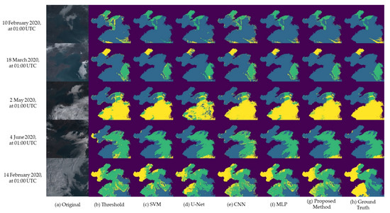
Figure 6.
Detection results of five different sea fog events occurred during 2020 using six different algorithms. Each row represents a sea fog event, and its observation time is displayed on the left. Each column represents: (a) original Himawari-8 images, (b) results of threshold method [12], (c) results of the SVM method, (d) results of the U-Net method, (e) results of the CNN, (f) results of the MLP, (g) results of the proposed method, (h) ground truth of the corresponding images of (a). The clouds, clear sky, and sea fog pixels are marked yellow, blue, and green, respectively.
4.3. Validation with CALIPSO VFM
Although the AHI has the characteristics of high spatial resolution and sustainable observation, providing a new level of capability for detecting sea fog, it fails to offer the cloud base height parameter for discrimination between low-level stratus and fog. The problem is particularly evident in ocean areas, where no ground observations are available [30]. The CALIOP was jointly developed by NASA (National Aeronautics and Space Administration) and CNES (French Centre National d’Etudes Spatiales) and became operational in 2006. The CALIOP has two bands of 532 nm and 1064 nm, which can penetrate clouds and aerosols and obtain atmospheric vertical profile structure information [31]. The Level 2 products of CALIOP, known as CALIPSO VFM products, provide information on cloud and aerosol locations and types. Although the CALIPSO VFM can fill the gap with the capability of vertical profiling, it does not always meet the needs, since it follows its orbit linearly rather than in real-time. Therefore, in this section, the VFM products were used to validate the fog detection accuracy of the proposed algorithm.
Figure 7a shows a sea fog case observed by Himawari-8 on 8 June 2018 05:10 (UTC) with CALIPSO passes over (solid white line) the study area at nearly the same time (8 June 2018 05:09:30–05:11:42 UTC). The detection result of our method illustrates that the sea fog almost fully covered the Yellow Sea and Bohai Sea area. Sea fog pixels were detected along the A-B, C-D, and E-F line segments, as displayed in Figure 7b. The CALIPSO VFM data demonstrate that there were clouds connected to the sea level (i.e., sea fog, according to the definition of fogs [32]) along three footprint line segments A-B, C-D, and south E-F in Figure 7c as well as rough surface (i.e., sea fog, identified as sea fog by [33,34,35]) located in the north half of E-F. These low-level clouds touching the sea surface identified by VFM data corresponded reasonably with the sea fog detection results of the proposed method. The CALIPSO also observed high clouds located at approximately 7–12 km in these three segments, which proves that the proposed method can detect the sea fog covered by transparent cirrus clouds to a certain extent. The validation experiment proved that our method has promising application for the detection of sea fog.
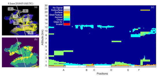
Figure 7.
The fog detection results and VFM validation of the proposed method. (a) The original Himawari-8 false-color image composited by band 04, band 05, and band 07, while the white solid line indicate the CALIOP orbit track; (b) the clear sky, clouds and sea fog regions detected by our model, corresponding to blue, yellow, and green colored pixels; (c) visualization of the VFM derived from the CALIPSO backscatter data along the footprint line on 8 June 2018, light blue, green, and orange indicate regions of “clouds”, “aerosols”, and “surface” with high confidence, respectively.
5. Conclusions
In this paper, we built a daytime sea fog dataset called YBSF that consisted of a sequence of AHI images with ground truth labels. A two-stage neural network-based sea fog detection method was presented and tested on the proposed dataset. The experimental results show that, compared with the traditional machine learning methods or classical neural network architectures, the two-stage neural networks algorithm achieved the highest accuracy for sea fog detection. Furthermore, the proposed method had excellent advantages in digging out the data connections between different channels through convolution networks, so that it does not need a careful selection of channel data for discriminatory input features, which eases the workload of analyzing and selecting channel combinations for meteorologists. Many researchers believe that partial channel combination thresholds can separate clear sky, clouds, and sea fog. However, we conducted a series of experiments and concluded that full channel data, instead of partial channel combination data, as input of data-driven algorithms, can outperform in detecting sea fog tasks. Further validation on the CALIPSO VFM data also confirmed that our method is effective for sea fog detection.
It should be noted that from the perspective of meteorological satellites, sea fog is often obscured by clouds above it. The existing methods including the proposed method fail to efficiently extract the fog area under cloud cover. Geostationary meteorological satellites can obtain time-dependent changes in the occlusion of fog by clouds through continuous observation. How to effectively use temporal information to extract sea fog under cloud cover will be the next research effort.
Author Contributions
Conceptualization, Y.T. and P.Y.; Methodology, Y.T.; Software, P.Y.; Validation, Y.T. and P.Y.; Formal analysis, Z.Z. and X.Z.; Writing—original draft preparation, Y.T. and P.Y.; Writing—review and editing, Z.Z. and X.Z.; Visualization, P.Y. All authors have read and agreed to the published version of the manuscript.
Funding
This research was funded by the National Natural Science Foundation of China, grant numbers 61473310, 41775027, and 42075139.
Data Availability Statement
The YBSF dataset is available at https://github.com/TangYuzhu/YBSF-dataset/tree/master (accessed on 13 September 2022). The VFM data are available at https://www-calipso.larc.nasa.gov/products/lidar/browse_images/std_v4_index.php (accessed on 13 September 2022).
Acknowledgments
We are grateful for the access to the satellite data at the JMA (for Himawari-8) and the NOAA (for VFM). We also thank the anonymous reviewers for their constructive comments.
Conflicts of Interest
The authors declare no conflict of interest.
References
- Pavolonis, M. GOES-R Advanced Baseline Imager (ABI) Algorithm Theoretical Basis Document for Volcanic Ash; Version 2; NOAA NESDIS Center for Satellite Applications and Research: Silver Spring, MD, USA, 2010. [Google Scholar]
- Hunt, G.E. Radiative properties of terrestial clouds at visible and infra-red thermal window wavelengths. Q. J. R. Meteorol. Soc. 1973, 99, 346–369. [Google Scholar] [CrossRef]
- Eyre, J.; Brownscombe, J.L.; Allam, R.J. Detection of fog at night using Advanced Very High Resolution Radiometer (AVHRR) imagery. Meteorol. Mag. 1984, 113, 266–271. [Google Scholar]
- Ellrod, G.P. Advances in the Detection and Analysis of Fog at Night Using GOES Multispectral Infrared Imagery. J. Weather Forecast. 1995, 10, 606–619. [Google Scholar] [CrossRef]
- Bendix, J.; Thies, B.; Cermak, J.; Nauß, T. Ground Fog Detection from Space Based on MODIS Daytime Data—A Feasibility Study. Weather Forecast. 2005, 20, 989–1005. [Google Scholar] [CrossRef]
- Sun, H.; Sun, Z.B.; Li, Y.C. Metorological Satellite Remote Sensing Spectral Charateristics of Fog. J. Nanjing Institule Meterorol. 2004, 27, 289–301. [Google Scholar] [CrossRef]
- Ma, H.Y.; Li, D.R.; Liu, L.M.; Liang, Y.T. Fog Detection Based on EOS MODIS Data. Geomat. Inf. Sci. Wuhan Univ. 2005, 30, 143–145. [Google Scholar]
- Hao, Z.Z.; Pan, D.L.; Gong, F.; Zhu, Q.K. Optical Radiance Characteristics of Sea Fog Based on Remote Sensing. Acta Opt. Sin. 2008, 28, 2420–2426. [Google Scholar] [CrossRef]
- Zhang, C.G.; He, J.D.; Ma, Z.G. Remote Sensing Monitor of Sea Fog in Fujian Coastal Region. Chin. J. Agrometeorol. 2013, 34, 366–373. [Google Scholar] [CrossRef]
- Zhang, S.P.; Yi, L. A Comprehensive Dynamic Threshold Algorithm for Daytime Sea Fog Retrieval over the Chinese Adjacent Seas. Pure Appl. Geophys. 2013, 170, 1931–1944. [Google Scholar] [CrossRef]
- Wu, X.; Li, S. Automatic sea fog detection over Chinese adjacent oceans using Terra/MODIS data. Int. J. Remote Sens. 2014, 35, 7430–7457. [Google Scholar] [CrossRef]
- Cermak, J.; Bendix, J. A novel approach to fog/low stratus detection using Meteosat 8 data. Atmos. Res. 2008, 87, 279–292. [Google Scholar] [CrossRef]
- Drönner, J.; Egli, S.; Thies, B.; Bendix, J.; Seeger, B. FFLSD—Fast Fog and Low Stratus Detection tool for large satellite time-series. Comput. Geosci. 2019, 128, 51–59. [Google Scholar] [CrossRef]
- Kim, D.; Park, M.-S.; Park, Y.-J.; Kim, W. Geostationary Ocean Color Imager (GOCI) Marine Fog Detection in Combination with Himawari-8 Based on the Decision Tree. Remote Sens. 2020, 12, 149. [Google Scholar] [CrossRef]
- Krizhevsky, A.; Sutskever, I.; Hinton, G.E. ImageNet Classification with Deep Convolutional Neural Networks. In Proceedings of the Neural Information Processing Systems-Volume 1, Lake Tahoe, NV, USA, 3–8 December 2012; pp. 1097–1105. [Google Scholar]
- Girshick, R.; Donahue, J.; Darrell, T.; Malik, J. Rich Feature Hierarchies for Accurate Object Detection and Semantic Segmentation. In Proceedings of the 2014 IEEE Conference on Computer Vision and Pattern Recognition, Washington, DC, USA, 23–28 June 2014; pp. 580–587. [Google Scholar]
- He, K.; Zhang, X.; Ren, S.; Sun, J. Spatial Pyramid Pooling in Deep Convolutional Networks for Visual Recognition. IEEE Trans. Pattern Anal. Mach. Intell. 2015, 37, 1904–1916. [Google Scholar] [CrossRef]
- Yuan, Y.; Lin, L. Self-Supervised Pretraining of Transformers for Satellite Image Time Series Classification. IEEE J. Sel. Top. Appl. Earth Obs. Remote Sens. 2021, 14, 474–487. [Google Scholar] [CrossRef]
- Si, G.; Fu, R.D.; He, C.F.; Jin, W. Daytime sea fog recognition based on remote sensing satellite and deep neural network. J. Optoelectron·Laser 2020, 31, 1074–1082. [Google Scholar] [CrossRef]
- Jeon, H.-K.; Kim, S.; Edwin, J.; Yang, C.-S. Sea Fog Identification from GOCI Images Using CNN Transfer Learning Models. Electronics 2020, 9, 311. [Google Scholar] [CrossRef]
- Simonyan, K.; Zisserman, A. Very Deep Convolutional Networks for Large-Scale Image Recognition. In Proceedings of the Learning Representations, San Diego, CA, USA, 7–9 May 2015; pp. 1–14. [Google Scholar]
- He, K.; Zhang, X.; Ren, S.; Sun, J. Deep Residual Learning for Image Recognition. In Proceedings of the 2016 IEEE Conference on Computer Vision and Pattern Recognition (CVPR), Las Vegas, NV, USA, 27–30 June 2016; pp. 770–778. [Google Scholar]
- Zhou, Y.; Chen, K.; Li, X. Dual-Branch Neural Network for Sea Fog Detection in Geostationary Ocean Color Imager. IEEE Trans. Geosci. Remote Sens. 2022, 60, 1–17. [Google Scholar] [CrossRef]
- Zhang, S.-P.; Xie, S.-P.; Liu, Q.-Y.; Yang, Y.-Q.; Wang, X.-G.; Ren, Z.-P. Seasonal Variations of Yellow Sea Fog: Observations and Mechanisms. J. Clim. 2009, 22, 6758–6772. [Google Scholar] [CrossRef]
- Wang, Y.; Gao, S.; Fu, G.; Sun, J.; Zhang, S. Assimilating MTSAT-Derived Humidity in Nowcasting Sea Fog over the Yellow Sea. Weather Forecast. 2014, 29, 205–225. [Google Scholar] [CrossRef]
- Binhua, W. Sea Fog; China Ocean Press: Beijing, China, 1983. [Google Scholar]
- Gao, S.; Lin, H.; Shen, B.; Fu, G. A heavy sea fog event over the Yellow Sea in March 2005: Analysis and numerical modeling. Adv. Atmos. Sci. 2007, 24, 65–81. [Google Scholar] [CrossRef]
- Bessho, K.; Date, K.; Hayashi, M.; Ikeda, A.; Imai, T.; Inoue, H.; Kumagai, Y.; Miyakawa, T.; Murata, H.; Ohno, T.; et al. An Introduction to Himawari-8/9— Japan’s New-Generation Geostationary Meteorological Satellites. J. Meteorol. Soc. Jpn. 2016, 94, 151–183. [Google Scholar] [CrossRef]
- Chunyang, Z.; Jianhua, W.; Shanwei, L.; Hui, S.; Yanfang, X. Sea Fog Detection Using U-Net Deep Learning Model Based On Modis Data. In Proceedings of the 2019 10th Workshop on Hyperspectral Imaging and Signal Processing: Evolution in Remote Sensing (WHISPERS), Amsterdam, The Netherlands, 24–26 September 2019; pp. 1–5. [Google Scholar]
- Yi, L.; Zhang, S.P.; Thies, B.; Shi, X.M.; Trachte, K.; Bendix, J. Spatio-temporal detection of fog and low stratus top heights over the Yellow Sea with geostationary satellite data as a precondition for ground fog detection—A feasibility study. Atmos. Res. 2015, 151, 212–223. [Google Scholar] [CrossRef]
- Winker, D.M.; Pelon, J.; Coakley, J.A.; Ackerman, S.A.; Charlson, R.J.; Colarco, P.R.; Flamant, P.; Fu, Q.; Hoff, R.M.; Kittaka, C.; et al. The CALIPSO Mission: A Global 3D View of Aerosols and Clouds. Bull. Am. Meteorol. Soc. 2010, 91, 1211–1230. [Google Scholar] [CrossRef]
- Gultepe, I.; Tardif, R.; Michaelides, S.C.; Cermak, J.; Bott, A.; Bendix, J.; Müller, M.D.; Pagowski, M.; Hansen, B.; Ellrod, G.; et al. Fog Research: A Review of Past Achievements and Future Perspectives. Pure Appl. Geophys. 2007, 164, 1121–1159. [Google Scholar] [CrossRef]
- Zhang, P.; Wu, D. Daytime Sea Fog Detection Method using Himawari-8 Data. J. Atmos. Environ. Opt. 2019, 14, 211–220. [Google Scholar] [CrossRef]
- Wu, D.; Lu, B.; Zhang, T.; Yan, F. A method of detecting sea fogs using CALIOP data and its application to improve MODIS-based sea fog detection. J. Quant. Spectrosc. Radiat. Transf. 2015, 153, 88–94. [Google Scholar] [CrossRef]
- Lu, B. CALIOP Sea Fog Detection and Its Application to the Daytime Modis Remote Sensing of Sea Fog. Master’s Thesis, Ocean University of China, Qingdao, China, 2015. [Google Scholar]


Publisher’s Note: MDPI stays neutral with regard to jurisdictional claims in published maps and institutional affiliations. |
© 2022 by the authors. Licensee MDPI, Basel, Switzerland. This article is an open access article distributed under the terms and conditions of the Creative Commons Attribution (CC BY) license (https://creativecommons.org/licenses/by/4.0/).