Capacity Estimation of Solar Farms Using Deep Learning on High-Resolution Satellite Imagery

Abstract

Global solar photovoltaic capacity has consistently doubled every 18 months over the last two decades, going from 0.3 GW in 2000 to 643 GW in 2019, and is forecast to reach 4240 GW by 2040. However, these numbers are uncertain, and virtually all reporting on deployments lacks a unified source of either information or validation. In this paper, we propose, optimize, and validate a deep learning framework to detect and map solar farms using a state-of-the-art semantic segmentation convolutional neural network applied to satellite imagery. As a final step in the pipeline, we propose a model to estimate the energy generation capacity of the detected solar energy facilities. Objectively, the deep learning model achieved highly competitive performance indicators, including a mean accuracy of 96.87%, and a Jaccard Index (intersection over union of classified pixels) score of 95.5%. Subjectively, it was found to detect spaces between panels producing a segmentation output at a sub-farm level that was better than human labeling. Finally, the detected areas and predicted generation capacities were validated against publicly available data to within an average error of 4.5% Deep learning applied specifically for the detection and mapping of solar farms is an active area of research, and this deep learning capacity evaluation pipeline is one of the first of its kind. We also share an original dataset of overhead solar farm satellite imagery comprising 23,000 images (256 × 256 pixels each), and the corresponding labels upon which the machine learning model was trained.

1. Introduction

1.1. Motivation

The sharp increase in photovoltaic panel adoption has resulted in photovoltaic installations becoming a key contribution to renewable energy production, first through residential deployment, and subsequently through commercial solar farms. The reasons for this significant rise include the global push for renewables (the UN Sustainable Development Goals being a recognizable example [1]), coupled with the steadily decreasing cost of each unit of electricity produced (the global average cost of renewable energy has dropped by 89% for solar equipment since 2009 [2]). Figure 1 shows the official numbers and targets of various countries over the last decade. There has been a clear exponential trend over the last two decades, going from 0.3 GW in 2000 to 3.5 GW in 2009 to 63.5 GW in 2019, and a forecast to reach 4240 GW by 2040 [2]). Currently, the global solar capacity doubles every 18 months [2]. It is estimated that at least $400 million is being invested annually into commercial solar energy generation [3]. The International Solar Alliance has 180 member countries as of 2022, and has committed one trillion dollars as an investment target [4].

The generation behavior of renewables such as solar and wind reflects the uncertainty and complexity of the natural world. The inherent decentralized nature of the deployment has resulted in a dearth of traceable data to better understand the demographic, geographic, and regional trends. Satellite imagery provides an opportunity to track this inherently decentralized deployment at scale and with granularity, objectivity, and in potential real-time, which could be an instrumental tool that informs both policymakers and industries of the state of PV deployment by region. Enhancing the diffusion of PV solar energy generation is aligned with the UN Sustainable Development Goals (SDGs), specifically goal 7—to “Ensure access to affordable, reliable, sustainable and modern energy for all”. Detailed asset-level data, including the spatial arrangement of installations, are particularly required to address the challenges of generation and planning faced by electricity system operators and electricity market operators and participants.

Existing databases of solar generating capacity are insufficient to address databasing needs because they are either aggregated (for example, those of the IEA2, IRENA3, or BP1), limited in geographical scope (for example, Google OpenPV, DeepSolar [5], or SolarNet [6]), or are not geospatially localized (for example, S&P Global World Electric Power Plant Database [2]), and/or are not publicly available for the research and policy community (for example, IHS’s Electric Plants).

This work aims to scientifically develop and test a globally generalizable approach for the detection and capacity evaluation of medium- and large-scale photovoltaic solar farms with state-of-the-art accuracy. This can be considered as a segmentation or pixel-level classification problem showing great potential for applying deep learning techniques to analyze remote sensing tasks. According to SolarNet [6], solar farm detection is more challenging than rooftop solar panel detection, because of the confusing backgrounds in which they are found. We use remote sensing and deep learning to detect solar farms—both their existence and precise boundaries—to estimate the energy generation capacities of individual facilities in an accurate manner, using publicly available satellite data and limited computational expense. These values are used to triangulate self-reported information, validate capacity figures, and even to identify real-world inefficiencies.

1.2. Previous Work

Identifying, understanding, and mapping renewables deployment is a topic that has gained interest in recent years. A variety of methods have been proposed to detect first residential and subsequently commercial photovoltaics from remote sensing images. Admittedly, rooftop detection is the more interesting case, given that they are more dispersed and not reported, but as commercial solar deployment becomes more widespread, the latter problem has developed into one of both intellectual and practical interest.

Stanford Deepsolar [5] kick-started interest in this field by proposing a deep learning framework to map residential rooftop solar panels for the US. DeepSolar utilized transfer learning to train a CNN classifier on imagery from Google Static Maps, and detected over 1.47 million PV installations in urban areas throughout the US with a precision of 93.1% and a recall of 88.5%. However, commercial solar deployment was not addressed by DeepSolar. Prior to that, rule-based efforts at detecting PV installations have not been able to achieve very high levels of precision and recall [7].

More recently, SolarNet [6] proposed an expectation maximization attention network to recognize solar farms on satellite imagery in China. In their paper, the authors compare the two most popular networks, UNet and EMANet, and combine the strengths of both to come up with their own SolarNet, which is a combination of the two. SolarNet was limited by geography and did not evaluate the capacity, or report semantic segmentation evaluation metrics such as the Jaccard Index. The detections by SolarNet and by Kruitwagen et al. [3] were at the bounding box/convex hull level for each solar farm. This is useful to achieve an upper bound on true solar capacity, but tends to overestimate the true solar capacity of an installation. Prior efforts also did not make the underlying data sets fully public.

1.3. Problem Statement

In this research, we seek to answer the following questions:

• How do we best use deep learning to extract detected polygon areas containing solar farms from satellite imagery?
• Apart from verifying the existence and geographic location of a solar farm, can we estimate the number of individual panels?
• What is the best way to use this information to predict how much solar energy is generated annually?

We show how to extract this information from satellite imagery and to validate both the detected areas and generation capacities against publicly available data, including the electricity generation data reported by solar farm management.

1.4. Contributions

In this paper, we propose, optimize, and validate a deep learning based framework to detect and map solar farms across different geographies using a state-of-the-art semantic segmentation convolutional neural network-based pipeline. Semantic segmentation enables the precise localization of solar panel areas from satellite imagery for a more accurate estimate of the deployment area. As a final step in the pipeline, we develop a multi-step capacity evaluation model to estimate the number of panels and the energy generation capacity of the detected solar energy facilities.

The final question of the problem statement addresses the real world consequential information that can be extracted from the output polygons of the model. We develop a capacity evaluation model that starts where the deep learning problem ends, and demonstrate on some sample solar farms, verifying against real-world reported data. Deep learning applied specifically for the detection and mapping of solar farms is an active area of research, and this deep learning capacity evaluation pipeline is the first of its kind. Prior work in using satellite and aerial imagery has estimated the solar farm size, but not its estimated annual energy production capacity.

In summary:

• We present a deep learning model capable of solar farm detection that achieves highly competitive performance metrics, including a mean accuracy of 96.87%, and a Jaccard Index (intersection over union of classified pixels) score of 95.5%.
• Subjectively, our model was found to detect spaces between panels and pathways between panel rows producing a segmentation output that is better than human labeling. This has resulted in some of the most accurate detections in comparison with the existing literature.
• We share the original, pixel-wise labeled dataset of solar farms comprising 23,000 images (256 × 256 pixels each) on which the model was trained.
• Finally, we propose an original capacity evaluation model—extracting panel count, panel area, energy generation estimates, etc., of the detected solar energy facilities that were validated against publicly available data to within an average 4.5% error.

2. Materials and Methods

The capacity evaluation pipeline proposed in this paper comprises dataset creation, the deep learning model, and the capacity evaluation model. Our deep learning model was trained on an original dataset created by collecting the satellite imagery of several major solar farms in the US, and tested on images of farms unseen by the model. Data augmentation and ablation studies were performed to check the model’s robustness to complex backgrounds and edge cases. This computationally intensive task of training was carried out with the help of the MIT Supercloud using a minimum of 2056 processors. Finally, the output polygons detected by the model were fed into the capacity evaluation model for further analysis.

2.1. Dataset

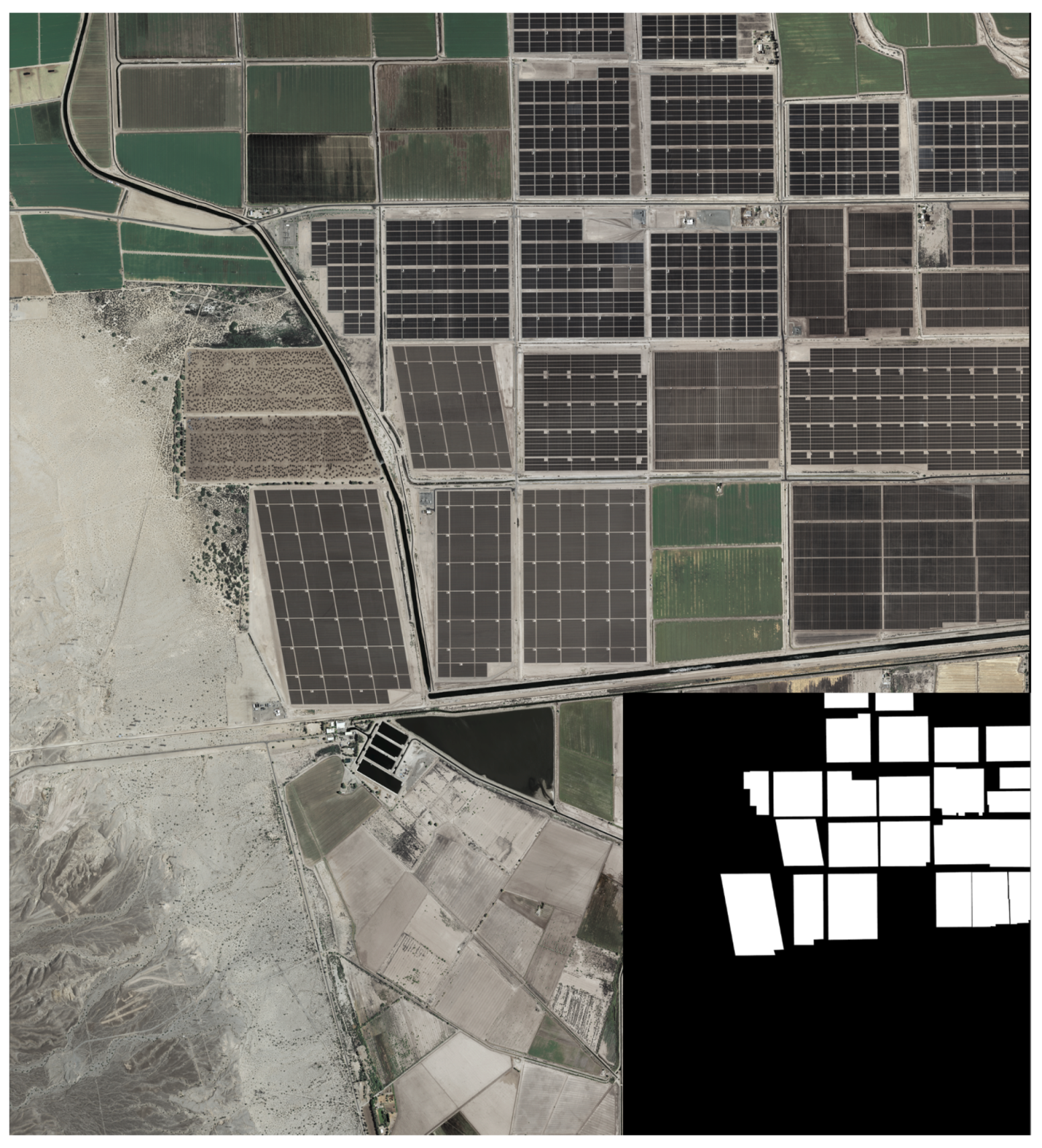
Seen in Figure 2 is what a typical solar farm looks like from space. The imperial county solar farm in Southeast California, close to the Mexico border, was all farmland in 2012, and has seen progressive development over the following years. Each of these images is a mosaic of geotiff tiles and serves as our source of data. Note that while it appears to be encroaching on farmland (one of the major criticisms of solar energy), the facility is actually in the middle of the arid Mojave desert and encroaching on highly irrigation intensive farms. The tradeoff in land use between farming and energy is an interesting use case but is beyond the scope of this paper.

The first step in the process was to evaluate the sources of satellite imagery suitable for building a dataset of labeled images on which to train and test a deep learning model. In order to create our own dataset of imagery for this purpose, a number of satellite imagery sources were explored, with the criteria being resolution and availability across geographies. Sources range from freely accessible satellite imagery, low-resolution imagery from publicly owned assets (such as NASA’s Landsat series of satellites), etc., to higher-resolution images from commercial resources like Planet, DigitalGlobe’s WorldView, or ArcGIS. For the needs of this project, the USDA NAIP repository [8] (0.6 m GSD) sourced via USGS Earth Explorer [9] was chosen for analysis and dataset creation because it satisfied both the criteria of adequate resolution and uniform availability across the US.

Overhead imagery was collected, and detailed annotation was carried out on 10 major solar farms across the US (the annotated imagery of a few solar farms is included in Appendix A for reference). Solar farm areas were manually labeled to be used as ground truth (this is machine learning terminology, not the remote sensing definition) This is known as annotation. Annotation encompasses the negative labeling of nearby agricultural, semi-urban, and topographical relief systems. This was achieved using an open source tool called QGIS that helps build on geotiff files and creates masks that were then used as ground truth. A visual representation of the labeling process that was involved in dataset creation is seen in Figure 3.

Next, the large geotiff imagery was patchified into 256 × 256 patches, forming the basis of our novel dataset (one of the contributions of this paper) of about 23,500 labeled images in total for training, validating, and testing. Certain solar farms were set aside in entirety for testing so that the model could be evaluated on solar farms previously unseen by the model.

Table 1. Composition of the dataset. Some labeled and unlabeled solar farms are reserved exclusively for testing as an additional check for robustness and generalizability. The labeled portion of the dataset consists of 23,500 images, along with their corresponding labels/masks ready for training.

Solar Farm	Location	Capacity (mW)	Train/Test	Images	Labels
Mount Signal	Imperial County, CA, 32${}^{°}$40${}^{\prime }$24${}^{″}$N, 115${}^{°}$38${}^{\prime }$23${}^{″}$W	1165	Train	4000	4000
Techren Solar	Boulder, NV, 35${}^{°}$47${}^{\prime }$N, 114${}^{°}$59${}^{\prime }$W	700	Train	2500	2500
Topaz Solar	San Luis Obispo, CA, 35${}^{°}$23${}^{\prime }$N, 120${}^{°}$4${}^{\prime }$W	550	Train	6000	6000
Copper Mountain Solar	El Dorado, NV 35${}^{°}$47${}^{\prime }$N, 114${}^{°}$59${}^{\prime }$W	298	Train	2500	2500
Desert Sunlight	Desert Center, CA, 33${}^{°}$49${}^{\prime }$33${}^{″}$N, 115${}^{°}$24${}^{\prime }$08${}^{″}$W	1287	Test	4500	4500
Agua Caliente	Yuma County, AZ, 32${}^{°}$57.2${}^{\prime }$N, 113${}^{°}$29.4${}^{\prime }$W	740	Test	4500	4000
Solar Star	Rosamond, CA, 34${}^{°}$49${}^{\prime }$50${}^{″}$N, 118${}^{°}$23${}^{\prime }$53${}^{″}$W	831	Test	4000	-
Springbok	Kern county, CA, 35.25${}^{°}$N, 117.96${}^{°}$W	717	Test	4500	-
Great Valley Solar	Fresno County, CA, 36${}^{°}$34${}^{\prime }$52${}^{″}$N, 120${}^{°}$22${}^{\prime }$46${}^{″}$W	200	Test	4000	-
Mesquite	Maricopa County, AZ, 33${}^{°}$20${}^{\prime }$N, 112${}^{°}$55${}^{\prime }$W	400	Test	2000	-

gives an overview of the composition of the dataset.

2.2. Dataset Augmentation

Ideally, a robust convolutional neural network (CNN) should be able to classify objects even when they are positioned in different orientations or translations. However, CNNs are not architecturally invariant to translation, size, or illumination. In fact, several studies have found that these networks systematically fail to recognize new objects in untrained locations or orientations [10].

This is where data augmentation becomes essential. We account for the amount and diversity of data by training a neural network with additional synthetically modified data without actually collecting or labeling new data. This means applying minor alterations and changes to our existing dataset so that variations of the training set images are more likely to be seen by the model, dramatically improving subsequent generalization.

In this study, we augmented our dataset using contrast matching to bring out subtle differences in shade and to create a higher contrast image, as well as some commonly used morphological transformations in image processing, such as random rotations in 45 and 90 degree increments, and flipping the image horizontally and vertically with a 50% probability.

It is observed that augmentation techniques play a positive role in precise detection. Qualitative effects of image augmentation can be observed in the figure in Section 3.3.

2.3. Deep Learning Model Architecture

The structure of this problem calls for the use of a pixel-wise classifier, otherwise known as a semantic segmentation convolutional neural network (CNN). Semantic segmentation enables the precise localization of solar panel areas from satellite imagery for the most accurate estimate of the deployment area. This is because the output is a mask, rather than just a classification or bounding box. A standard CNN can classify a full image as containing a certain object. A bounding box level classifier will localize the detected object to within a square or rectangular box. A pixel-to-pixel classifier, however, can identify which pixel(s) of the image contains the object of interest, thus resulting in an output polygon of arbitrary shape. Since we are interested in the exact panel area of facilities, a pixel-level classifier can give us the most accurate area estimate. Similar problems have been addressed in [11,12] that used semantic segmentation convolutional neural networks for various purposes. The architecture of a CNN for semantic segmentation differs from the classification/bounding box CNNs, in that the output is at the pixel level. The choice to use such a CNN comes with the additional burden of requiring pixel-to-pixel labels for the datset. A semantic CNN also needs less data to train because the training labels specify exactly what to look for in the imagery.

An established CNN used as a benchmark semantic segmentation model is known as the “UNet”, which is a traditional patch classification method first proposed in 2014. It gets its name from its architecture (U shaped) that contains two paths. The first path is the contraction path (also known as the encoder), which is used to capture the context in the image. The second path is the symmetric expanding path (also known as the decoder), which is used to enable precise localization. This is how U-Net combines low-level detail information and high-level semantic information. This architecture produces a prediction for each pixel, while retaining the spatial information in the original input image. The key to doing this is to change the last step of a CNN, making it fully convolutional instead of fully connected. This is why the UNet is an FCN (fully convolutional network), not a CNN (convolutional neural network).

Figure 4 visualizes the generalized architecture of UNet. It is similar to a CNN at every layer, except the final step, which is a 1 × 1 convolution used to map the channels to the desired number of classes retaining the pixel-to-pixel structure in the output. For comparison, a convolutional neural network (CNN) adopts the fully connected layer to obtain fixed-length feature vectors for classification. Instead of this, the deconvolution layer of FCN performs the feature map of the last volume-based layer. The UNet architecture that stems from FCN is used as a baseline model, and the network architecture is illustrated in Figure 4.

For this research, a deep learning model was developed using the open-source PyTorch library running in Python 3.7. We chose a UNet architecture with F = 64, which gives us a model with 1,940,000 trainable parameters—F was initially chosen based on the literature, and the parameters were finetuned until the best metrics were achieved. All FCN architectures explored were common in their utilization of normalized CMYK satellite images as input.

2.4. Model Evaluation

In order to properly train and test the proposed segmentation method, training images are generated by cropping the large original image tiles into patches of “digestible size”, and these are fed into the network to learn the parameters. For deployment on larger images during the testing phase, the output masks can be stitched together as depicted in Figure 5, to conform with the input image, no matter the size. No data augmentation was used during initial training. The model was trained with an empirically optimal minibatch size of 10. The learning rate was initially set to 0.001 and then reduced to 0.1. The network converged in roughly 20–30 epochs.

The metrics for evaluating any semantic segmentation model differ slightly from those of a CNN used for classification problems. Rather than precision and recall (completeness and correctness), insight is gleaned from metrics called pAcc (pixel accuracy), mAcc (mean accuracy), and the Intersection over Union (IoU)/Jaccard index.

Pixel accuracy is a metric that denotes the percent of pixels that are accurately classified in the image. This metric calculates the ratio between the amount of adequately classified pixels and the total number of pixels in the image as

$$pAcc=\frac{correctlyclassifiedpixels}{totalpixels}$$

The mean accuracy is a metric that denotes the percent of images that are accurately classified in the dataset. This metric calculates the ratio between the amount of adequately classified images and the total number of images in the image as

$$mAcc=\frac{correctlyclassifiedimages}{totalimages}$$

In semantic segmentation, a correctly classified image is hard to define. It is typically a threshold, say, more than half of the image is correctly segmented. As a consequence, poor detections can pass through this metric, making it more generous and less informative than what is needed. The most exacting metric is the intersection over union score, also known as the Jaccard similarity coefficient, a statistic that is used for gauging the similarity of the detected shape against its label.

$$IoU=\frac{A\cap B}{A\cup B}$$

2.5. Capacity Evaluation Model

In order to maximize utility to stakeholders, the final step in the proposed pipeline—the capacity evaluation model—explores the extraction of further information from remotely sensed solar energy facilities. Beyond verifying the existence and geographic location of the farms, can we estimate or count the number of panels? How do we predict how much solar energy is generated annually? These values can be used to triangulate self reported information, validate capacity figures, and even identify real-world inefficiencies.

The capacity evaluation model proposed in this section is a compound model of three independent steps—the accurate estimation of deployment area, the estimate of the number of panels, and finally, the evaluation of the energy production capacity of the facility. As depicted in Figure 6, the polygons detected via a deep learning pipeline are used to estimate the “convex hull” area of the facility. Next, the area estimate is distilled down to an estimate of panel area, and consequently, the number of panels. Finally, the energy production capacity is evaluated using a standard formula that includes efficiency, location (weather effects), and/or capacity factor. The area estimate hinges on model accuracy and quality of imagery; the estimate of the number of panels depends on panel dimensions, packing density, and axis system type. Finally, the energy production number depends on capacity factor, which in turn is governed by location, weather effects, panel efficiency, and so on.

Two approaches are explored to arrive at a capacity estimate. The first is a formula that uses a published capacity factor for a given geographic location, or the farm itself, if the number is available. The second, more complex method independent of assumptions, is based on NREL’s PySAM model [13].

The capacity factor (CF), used in the first method, is defined as the ratio of actual energy delivered over a period of time over the maximum possible as per the rated capacity of a power plant operating non-stop. The typical capacity factors of most farms in the world range between 30 and 40%, while those in the Mohave desert are more specifically clustered at around 33–37%. CF depends on the geographic location and varies based on the actual weather events for a particular year.

$$CapacityFactor=\frac{AnnualEnergyProduction(\mathrm{k}\mathrm{W}\mathrm{h}/\mathrm{y}\mathrm{e}\mathrm{a}\mathrm{r})}{SystemRatedCapacity(\mathrm{k}\mathrm{W}\mathrm{h}/\mathrm{h})\times 24(\mathrm{h}/\mathrm{d}\mathrm{a}\mathrm{y})\times 365(\mathrm{d}\mathrm{a}\mathrm{y}\mathrm{s}/\mathrm{y}\mathrm{e}\mathrm{a}\mathrm{r})}$$

(1)

Alternately, a more complex route may be taken that is independent of assumptions, and that is based on NREL’s PySAM model. NREL’s PySAM model uses a large number of criteria, including actual hourly meteorological data (horizontal irradiance, normal irradiance, diffuse irradiance, dew point, surface albedo, temperature, relative humidity, solar zenith angle...) to arrive at the energy generated by a panel on a given day. This estimate can then be fed into the model to calculate the actual annual production instead of the capacity factor method, which is an extrapolation from day to year.

The methodology is visualized in Figure 6, and step-by-step calculations and results are elaborated in the tables in Section 3.4. The method is as follows: first, the polygons detected by the deep learning pipeline are used to estimate the “convex hull” area of the facility, which is brought down to panel area using a packing density. The model accuracy, resolution of imagery available, and quality of imagery directly affect this number. Next, the area estimate is distilled down to an estimate of the panel area, and consequently, the number of panels.

$$NumberofPanels=\frac{TotalPanelArea}{AreaperPanel}$$

(2)

$$\Rightarrow NumberofPanels=\frac{NumberofPixels\times (Area/Pixel)\times PackingDensity}{AreaofPanel}$$

(3)

Ultimately, the energy production capacity is evaluated using Equation (1) as:

$$AnnualCapacity(\mathrm{k}\mathrm{W}\mathrm{h}/\mathrm{y}\mathrm{e}\mathrm{a}\mathrm{r})=CF\times SystemRatedCapacity\left(\mathrm{k}\mathrm{W}\right)\times 24\times 365$$

(4)

where,

$$SystemRatedCapacity\left(\mathrm{k}\mathrm{W}\right)=PanelRatedCapacity\left(\mathrm{k}\mathrm{W}\right)\times NumberofPanels$$

(5)

3. Results

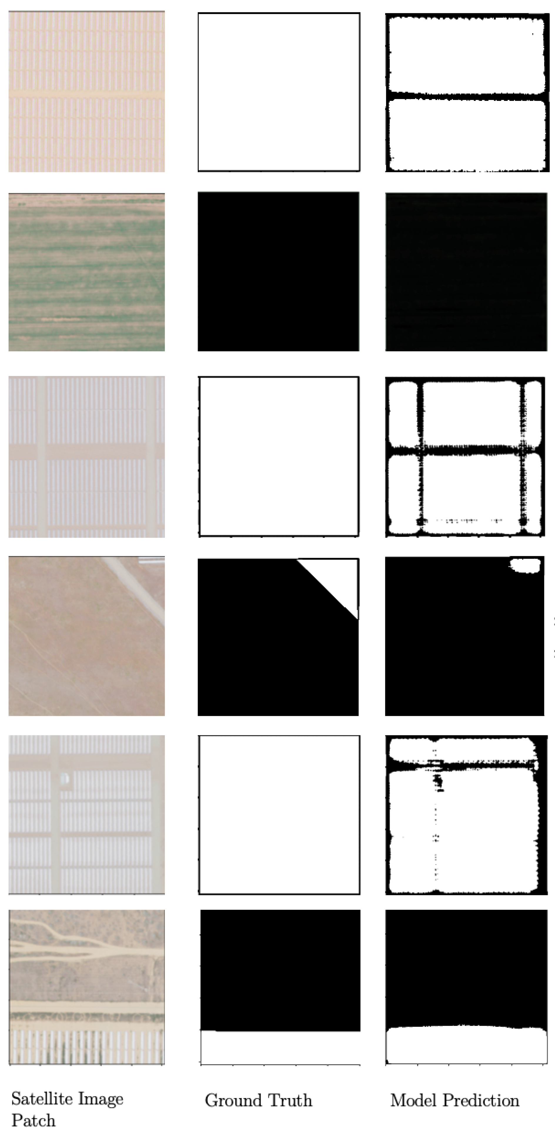
Summarized in

Table 2. Results—key performance metrics of the CNN.

Metric	Description	Result
pAcc (Pixel Accuracy)	Correctly classified pixels/total pixels	99.19%
mAcc (Mean Accuracy)	Mean accuracy considering optimal threshold	96.87%
mIoU (Mean IoU/Jaccard Index)	Overlap between mask and prediction	95.5%
fIoU (Frequency corrected IoU)	IoU reported for each class and weighted	97%

are the performance metrics achieved by our best model. Our best performing model produced a semantic segmentation output that is better than human labeling, and the patches can be seen in Figure 7. The segmentation performance on various full solar farms can be seen in Figure 8.

3.1. Performance Metrics

The best performing model achieved a mean accuracy of 96.87% and an mIoU of 95.5%. For comparison, solarNet achieved an mIoU score of 94.2%. The high IoU score is supported by Figure 7 and Figure 8, which illustrate how the model is able to identify nuances within the solar farm at a sub-farm level, such as spaces between panel rows, pathways, and maintenance blocks.

3.2. Effect of Confidence Threshold

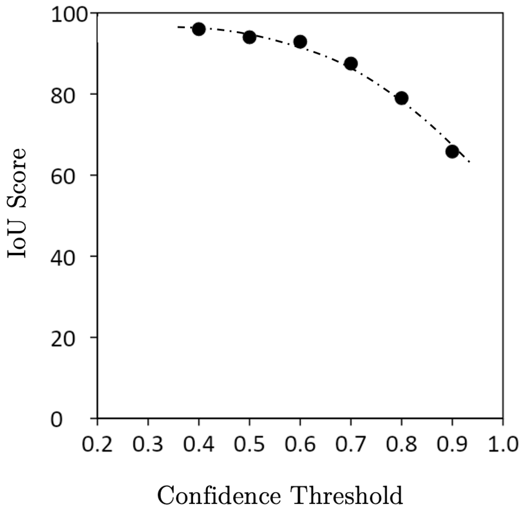
The IoU threshold is the confidence value at which a pixel is considered to be classified as containing photovoltaics. In standard practice, >0.5 confidence is considered as a positive prediction. A classification threshold is analogous to saying that there are higher/lower standards for accepting a pixel as yes/no. Seen in Figure 9 is the variation of the IoU score with the IoU threshold. As expected, there is a decline as the cutoff is made tighter. This can be interpreted in two ways. One, that the model is confident in its predictions, as IoU score only drops fast as the cutoff approaches 1. The best IoU score, 95.5%, was achieved with a cutoff at 0.4, which means the model is balanced but slightly more confident of negative predictions.

3.3. Effect of Image Augmentation

It can be qualitatively observed from Figure 10 that the augmentation techniques play a positive role in precise detection. As seen in Figure 10, the model detections are noisy before training the model on the augmented images. The results after applying the augmentation techniques (elucidated in the Methodology section) show that augmentation not only reduced the amount of noise, but was able to progressively help the model learn the essence of a solar farm.

3.4. Capacity Evaluation

The previous sections have affirmed our ability to input satellite imagery and extract detected polygon areas containing solar farms using a deep-learning-based pipeline. The capacity evaluation model developed in this paper comprises three pieces—the accurate estimation of the deployment area, the estimate of the number of panels, and finally, the evaluation of the energy production capacity of the facility. These steps are visualized in the model diagram in Figure 6, and are enumerated and presented in

Table 3. Area Detection—the first step in capacity evaluation. Note that detected area is purely panel outlines while reported area includes peripheral area.

Solar Farm	Pixels Counted $\mathit{Mil}$	Area Detected (km${}^2$)	Area Reported (km${}^2$)	Panel Area (km${}^2$)
Mount Signal	34.27	12.34	15.9	4.93
Agua Caliente	21.65	7.79	9.7	3.12
Desert Sunlight	38.53	13.87	16	5.55
Solar Star	25.33	9.12	13	3.65
Springbok	18.33	5.52	5.7	2.21

,

Table 4. Estimate of the number of panels. The panel area is converted into panel count, taking into account the type of panels in the farm and their corresponding dimensions.

Solar Farm	Panel Type	Panel Area (km${}^2$)	# Panels Counted $\left(\mathit{Million}\right)$	# Panels Reported ($\mathit{M}\mathit{i}\mathit{l}\mathit{l}\mathit{i}\mathit{o}\mathit{n}$)	Error (%)
Mount Signal	FS 3&4	4.93	6.85	6.8	<1%
Agua Caliente	FS S4	3.12	4.33	4.8	9.7%
Desert Sunlight	FS S4	5.55	7.71	8.0	3.6%
Solar Star	Sunpower	3.65	1.55	1.7	8.8%
Springbok	FS S4	2.21	3.07	3.0	2.3%

and

Table 5. Capacity calculation results. We report the average of the two error values for each solar farm, which lies in the range 2–7%.

Solar Farm	# Panels Counted	# Panels Reported	Annual Capacity Calculated (GWh)	Annual Capacity Reported (GWh)	Capacity Evaluation Error (%)	Max (Errors) (%)
Mount Signal	6.85	6.8	1165.1	1197	2.7%	2.7%
Agua Caliente	4.33	4.8	736.0	740	<1%	9.7%
Desert Sunlight	7.71	8.0	1309.9	1287	1.8%	3.6%
Solar Star	1.45	1.7	861.2	831	3.7%	8.8%
Springbok	3.07	3.0	623.2	717	13.1%	13.1%

.

Illustrated in the following tables are some case studies of the model applied to US solar farms. The results are presented step-by-step and are compared with reported numbers. Table 3 depicts the area detection, the first step in the capacity evaluation pipeline. The pixel count is multiplied by the square of the resolution (0.36 (m${}^2$)) to arrive at the area estimate. Note that the differences between the detected area and the reported area are accounted for by the fact that the detected area comes from purely panel outlines detected by the CNN, whereas the reported area is a number from a commercial point of view—the area operated by farm management—and therefore, includes peripheral area, ongoing work, pathways, etc.

Table 4 depicts the estimate of the number of panels. The panel area is converted into panel count by taking into account the types of panels in the farm and their corresponding dimensions. This is because “number of panels” itself is not as relevant as total photovoltaic area. The difference in numbers is likely also caused in part due to somewhat incorrect data itself—the precise outlines of farms are dynamic, and reporting nomenclature can change as they are influenced by financial factors, taxation, timing, ownership change, etc.

Finally, Table 5 shows the capacity calculation results using capacity factors that are relevant to the geographical location of the farm. While the model ultimately gives fairly close estimates overall (all within 10%), there is notable variation between farms. There is a case of the capacity evaluation error percentage being low, despite panel estimates not being as precise (Agua Caliente), and vice versa (Springbok). Hence, the maximum of the two errors is also reported. This variation in numbers could be attributed to temporal factors—solar farms are dynamic and changing, whereas the reported figures are true for a point in time. Time changes, weather variations, and nuances have not been considered in our model, whether in panel count, capacity factor, or annual generation.

4. Conclusions

The intersection of remote sensing and deep learning presents an exciting opportunity for geographically quantifying photovoltaic system deployment, essentially giving us the ability to draw insights on insofar lumped data. Insights from the remote quantification of photovoltaic deployment could have outcomes such as strategic decision-making, the cross-verification of reported data, and the incentivization of renewables targeting underserved territories.

This work explored several independent elements of a capacity pipeline that goes from raw overhead imagery to annual energy generation estimates by creating a dataset, labeling it, choosing a neural network, and training, testing, and optimizing the model for performance, and finally, by using results from the deep learning model to extract panel count, panel area, and capacity predictions of the detected solar energy facilities. Some of the key takeaways of this study are:

• A semantic segmentation model that achieved strong performance metrics including a mean accuracy of 96.87%, a Jaccard Index of 95.5% (compared to SolarNet’s 94.2%), and that is capable of highly precise and detailed detections. This has resulted in arguably some of the most precise/accurate solar farm detection imagery in the literature.
• An original, pixel-wise labeled dataset of solar farms that was sourced, annotated, and built for this problem, comprising 23,000 256 × 256 images on which the model was trained.
• A capacity evaluation model to extract panel count, panel area, energy generation estimates, etc., of the detected solar energy facilities that were validated against publicly available data to within 10% error, and an average error of 4.5%.

Future Work

There is plenty of scope for future work on this problem, as well as to the broader problem of applying remote sensing to renewable energy technology. This work fits into a longer-term goal of creating a granular global database of solar energy capacity production that could serve as a single source of truth for industries and policymakers to identify underserved areas and to inform decision-making. In the future, a highly refined version of this model could even be used as a replacement for conventional sources of knowledge, or as a secondary source of intelligence for the cross-validation of reported figures. We identify certain directions that future efforts at extending this research could take. They can be segmented as follows.

• Exploring newer neural net architectures and conducting a more detailed optimization study.
• Exploring other data sources, including hyperspectral imagery.
• Testing the performance of the CNN on data from other countries, incorporating additional training data if necessary. What remains to be conducted is automatic deployment on large geographical areas such as states and countries.
• Improving the accuracy and robustness of the capacity model. We were able to arrive at reasonably close estimates of solar farm areas, numbers of panels, and even the annual energy generated, but they are inconsistent. We enumerated some of the possible reasons for inconsistency that had to do with temporal changes, reporting, and data collection. With cleaner and more reliable data to compare to, the parameters/constants in the model, such as packing factor, can be updated with a least squares fit.
• Identifying trends and consequently underserved areas with high solar energy potential. The CNN can be deployed on the imagery of various regions to assess the deployment of commercial PV over time, and garner insights regarding the impacts of historical political, social, and economic factors on the deployment of solar renewable energy technology at scale.
• Identifying solar panel defects such as cracked solar cells, broken glass, and dust/sand build-up: defects in solar panels are unlikely to be detectable with imagery at a resolution of 0.4–0.7 m, so this will have to be completed with drone imagery.

References

1. Chu, S.; Majumdar, A. Opportunities and challenges for a sustainable energy future. Nature 2012, 488, 294–303. [Google Scholar] [CrossRef] [PubMed]
2. BP Statistical Review of World Energy 2018: Two Steps Forward, One Step Back | News and Insights | Home. Available online: https://www.bp.com/en/global/corporate/news-and-insights/press-releases/bp-statistical-review-of-world-energy-2018.html (accessed on 10 October 2022).
3. Kruitwagen, L.; Story, K.T.; Friedrich, J.; Byers, L.; Skillman, S.; Hepburn, C. A global inventory of photovoltaic solar energy generating units. Nature 2021, 598, 604–610. [Google Scholar] [CrossRef] [PubMed]
4. International Solar Alliance. Available online: https://newsroom.unfccc.int/news/international-solar-alliance (accessed on 10 October 2022).
5. Yu, J.; Wang, Z.; Majumdar, A.; Rajagopal, R. DeepSolar: A Machine Learning Framework to Efficiently Construct a Solar Deployment Database in the United States. Joule 2018, 2, 2605–2617. [Google Scholar] [CrossRef] [Green Version]
6. Hou, X.; Wang, B.; Hu, W.; Yin, L.; Wu, H. SolarNet: A Deep Learning Framework to Map Solar Power Plants In China From Satellite Imagery. arXiv 2019, arXiv:1912.03685. [Google Scholar]
7. Malof, J.M.; Bradbury, K.; Collins, L.M.; Newell, R.G. Automatic detection of solar photovoltaic arrays in high resolution aerial imagery. Appl. Energy 2016, 183, 229–240. [Google Scholar] [CrossRef] [Green Version]
8. National Agriculture Imagery Program (NAIP). Available online: https://naip-usdaonline.hub.arcgis.com/ (accessed on 10 October 2022).
9. Science for a Changing World. Available online: https://www.usgs.gov/ (accessed on 10 October 2022).
10. Biscione, V.; Bowers, J.S. Convolutional Neural Networks Are Not Invariant to Translation, but They Can Learn to Be. arXiv 2021, arXiv:2110.05861. [Google Scholar]
11. Agnew, S.; Dargusch, P. Effect of residential solar and storage on centralized electricity supply systems. Nat. Clim. Chang. 2015, 5, 315–318. [Google Scholar] [CrossRef]
12. Ekim, B.; Sertel, E. A Multi-Task Deep Learning Framework for Building Footprint Segmentation. In Proceedings of the 2021 IEEE International Geoscience and Remote Sensing Symposium IGARSS, Brussels, Belgium, 11–16 July 2021. [Google Scholar] [CrossRef]
13. NREL-PySAM—NREL-PySAM 3.0.0 Documentation. Available online: https://nrel-pysam.readthedocs.io/en/latest/version_changes/3.0.0.html (accessed on 10 October 2022).
Figure 1. Growth of global photovoltaic capacity has been exponential over the last two decades, from 0.3 GW in 2000 to 63.5 GW in 2019, roughly doubling every 18 months [2,3].
Remotesensing 15 00210 g001
Figure 2. Growth of Mount Signal Solar in Imperial Valley, California, into one of the world’s largest solar farms, over the last decade. Satellite imagery allows for a qualitative and quantitative “big picture” view of solar farms.
Remotesensing 15 00210 g002
Figure 3. The dataset annotation process.
Remotesensing 15 00210 g003
Figure 4. UNet architecture for solar farm detection. F = 64.
Remotesensing 15 00210 g004
Figure 5. Postprocessing—hundreds of individual images were stitched together to visualize detected solar farm areas.
Remotesensing 15 00210 g005
Figure 6. Depiction of the capacity evaluation model for solar farms. The goal is to estimate annual energy generation from polygons detected by the deep learning model on remotely sensed imagery.
Remotesensing 15 00210 g006
Figure 7. Predictions on individual patches (before postprocessing) show clearer outputs than human labeling (ground truth).
Remotesensing 15 00210 g007
Figure 8. Segmentation performance on various test solar farms. Comparison of the confidence masks between teacher confidence (in black and white) and the student confidence (in color) shows that the model produces an output with better veracity than human labeling.
Remotesensing 15 00210 g008
Figure 9. The variation of IoU score with confidence cutoff/threshold.
Remotesensing 15 00210 g009
Figure 10. Visualization of early improvement in the model with image and dataset augmentation.
Remotesensing 15 00210 g010