Groundwater Level Data Imputation Using Machine Learning and Remote Earth Observations Using Inductive Bias

Abstract

Sustainable groundwater management requires an accurate characterization of aquifer-storage change over time. This process begins with an analysis of historical water levels at observation wells. However, water-level records can be sparse, particularly in developing areas. To address this problem, we developed an imputation method to approximate missing monthly averaged groundwater-level observations at individual wells since 1948. To impute missing groundwater levels at individual wells, we used two global data sources: Palmer Drought Severity Index (PDSI), and the Global Land Data Assimilation System (GLDAS) for regression. In addition to the meteorological datasets, we engineered four additional features and encoded the temporal data as 13 parameters that represent the month and year of an observation. This extends previous similar work by using inductive bias to inform our models on groundwater trends and structure from existing groundwater observations, using prior estimates of groundwater behavior. We formed an initial prior by estimating the long-term ground trends and developed four additional priors by using smoothing. These prior features represent the expected behavior over the long term of the missing data and allow the regression approach to perform well, even over large gaps of up to 50 years. We demonstrated our method on the Beryl-Enterprise aquifer in Utah and found the imputed results follow trends in the observed data and hydrogeological principles, even over long periods with no observed data.

1. Introduction

Groundwater plays an important role in sustainable water resource management and comprises 30.1% of Earth’s freshwater use [1]. In the United States, 349 billion gallons of fresh water is used every day; groundwater makes up approximately 79.6 billion gallons—or approximately 26% of that total [2]. Humanity’s existence depends on monitoring and sustainably managing this important resource, yet we have a poor understanding of the spatial and temporal changes in groundwater storage [3].

Variations in groundwater levels, measured by sampling monitoring wells, provide a direct measure of groundwater levels and conditions. If monitored over time, these measurements can be used to characterize aquifer sustainability and availability. Important information about aquifer dynamics can be inferred from groundwater-level time series [4]. Groundwater-level observations are difficult to obtain, manage, archive, and distribute consistently, especially over longer time periods. Often, groundwater observation data are irregularly measured in both space and time because collection devices break, or wells stop being measured altogether. In the United States, there are over 800,000 groundwater monitoring sites, yet groundwater observation data remain sparse at many locations. On average, in the United States, each site has 10.1 records, which is only one measurement every 1–3 years on average [5]. The temporal sparsity of in situ observations, caused by irregularly collected data, makes it challenging to analyze the state of an aquifer, determine water availability and safe yields, forecast groundwater-level changes, or develop sustainable management plans.

Ignorance of safe aquifer yields can lead to over-pumping and, in turn, cause aquifer depletion; ground subsidence; and stress or death to local trees, wildlife, and fish [6]. Insufficient groundwater observation data make it difficult to assess the state of an aquifer to determine if storge is increasing, remaining stable, or decreasing. This knowledge is required to develop sustainable use strategies. In recent years, organizations such as the National Aeronautics and Space Administration (NASA) SERVIR program have increased their interest in monitoring groundwater by using remote Earth observations to better understand groundwater usage worldwide, provide insight in regions or areas with sparse data, and share groundwater information with users and managers to make informed management decisions. The objective of one of our research areas is characterizing groundwater resources in West Africa, where in situ measurements are particularly scarce. It is difficult to characterize groundwater levels by using Earth observations, but many of the processes that can be monitored by remote-sensing approaches are correlated with groundwater levels and use patterns, though these correlations may be limited to specific areas or regions, or even single wells [7,8]. We leverage these correlations, along with any existing measurements, to impute missing data and create records that can be used to characterize general aquifer storage and trends over longer time periods.

1.1. Previous Work

There are numerous methods to characterize an aquifer with sparse groundwater observations. One approach is to use physical-based numerical models to characterize groundwater flow in an aquifer. However, these physical-based models take a significant effort to develop and require detailed knowledge of the subsurface data to define physical structure and boundary conditions, and groundwater observations within the aquifer to calibrate and validate the model. These data are difficult to obtain, as groundwater measurements, geologic structure, and material properties, along with estimates of boundary conditions and sources or sinks, are required [9]. In many situations, this approach is impractical because of limited data and geologic information.

Recently, researchers have demonstrated that gaps in well observation data can be imputed by using regression approaches implemented with advanced statistical methods and machine-learning algorithms. These statistical models have weaknesses such as overfitting, low generalization, and limited predictive capability. However, based on the speed and relative accuracy of these approaches, researchers have found them to be a suitable alternative to traditional numerical groundwater models for data imputation [10].

A survey of neural network architectures for groundwater-level imputation and forecasting was conducted as early as 2001 and found a range of approaches, such as multi-layer perceptron (MLP), recurrent neural networks, and radial basis functions, being reported [11]. Since then, many other approaches have been reported, including support vector machines [12] adaptive neuro-fuzzy inference systems [13], and wavelet analysis [14]. Seasonal demands and recharge result in periodic aquifer behavior, so time-series analysis methods such as autoregressive integrated moving average have also been used to impute missing data and characterize aquifer behavior [15]. Researchers have also used convolutional neural networks to analyze the change of groundwater on large regional scales, using data from the Gravity Recovery and Climate Experiment (GRACE) sensors; these data, while generally regional in nature, can be used to help characterize changes and impute missing data for individual wells [16].

Researchers have observed that groundwater levels are influenced by meteorological events such as drought or wet years [17,18,19,20]. For example, during a drought, groundwater levels drop because of less recharge and more pumping as surface water sources are reduced. Conversely, during a wet period, generally groundwater levels rise due to a net increase in recharge and reduced groundwater extraction, as surface water resources are easier to exploit. However, this is a loose correlation with its own issues on which we later expand on in this paper. Nevertheless, Earth observations related to drought indicators such as soil moisture can be used as independent regression parameters to train models and exploit correlations with water levels [7].

Evans et al. [21] successfully leveraged these correlations between groundwater levels in wells and Earth observations to impute gaps in sparse water-level records. Their work demonstrated that each well or groundwater sample location has unique characteristics, and therefore, a model should be developed for each well, rather than developing an aquifer wide or regional model. They showed that large periods of missing groundwater observations could be imputed by regressing Earth observation data on groundwater measurements by using an Extreme Learning Machine neural network to fit regression equations for large gaps, while small gaps could be filled by using piecewise cubic Hermite interpolating polynomial (PCHIP) interpolation [21]. PCHIP is a standard interpolation method used to interpolate hydrology data without exceeding data maxima or minima, often called “overshoot” and “undershoot” [22,23,24]. The method proposed by Evans et al. [21] is a combination of interpolation for small gaps and regression for large gaps. For regression and large gaps, it treats every observation as an independent value and does not consider autocorrelation in time. For large gaps, the method of Evans et al. [21] fits the regression equations on existing measurements and meteorological data and then imputes or predicts missing values by using only the existing independent meteorological data, rather than auto-regressing the observation data from the groundwater-level time series they are imputing. This differs from time-series analysis methods because it does not use time correlations or lags to extrapolate missing values from existing data, though it does use smoothing algorithms on input data to capture some time correlations.

The Evans et al. [21] approach has a few limitations. Their approach assumes that the correlations between the groundwater-level data and the meteorological data at an individual groundwater well are strong enough to impute the missing data. However, this correlation between meteorological conditions and groundwater levels is very loose and does not represent causation. Short-term periodicity and trends in meteorological data, such as temperature or precipitation, may not be correlated with groundwater levels and cannot inform the regression models about various trends or periodicity in the groundwater levels at a given well. Their method works well for small uniformly distributed gaps and when general trends in the groundwater-level data are apparent from the historical observations. This assumption does not hold when data are available only in portions of the record, such as at the beginning or end, and the overall shape and trends of the data are not obvious.

1.2. Research Objective

Our research goal was to develop a method to impute or estimate groundwater levels that use globally available long-term datasets and exploit existing measured groundwater-level data to better capture periodic behavior and long-term trends.

We present a method to impute missing groundwater surface elevations at individual wells based on machine-learning regression, using in situ groundwater data from the target well, land-surface models, and remote Earth observations. Our method generates complete well records that can be used to analyze trends or other aquifer behaviors that otherwise would be difficult if not impossible to characterize by capturing periodicity and aquifer-specific trends by using any available in situ measurements at the well. If applied to all wells in an aquifer, this method can be used to characterize aquifer sustainability.

Our method is a modification and extension of the Evans et al. [21] method. We generated separate regression models for each well within an aquifer based on correlations with remote Earth observations and then used these regression models to impute missing data. We extended the Evans et al. [21] approach by building initial priors and encoding the time for each existing measurement. We developed priors at each well that represent the general non-linear trends we expected the well to have experienced, based local conditions and historical water use. These priors bias the model to prefer a hypothesis that better represents groundwater hydraulics and produces better imputation results over large gaps when there are no in situ data to indicate or constrain trends or features in the data. We encoded the month of the measurement and converted the measurement date to a value from 0 to 1 over the length of the imputation period. We then used these as independent features in the regression model, so the model can learn annual periodicity associated with months and trends associated with time (i.e., years).

In the following section of this paper, we provide details on the methods we used to extend Evans et al. [21]; describe the data used, generated features, and how these features were generated; and supply the processing details for our technique. We present and demonstrate our method with a case study that uses the Beryl-Enterprise aquifer, as it has long-term complete data records that can be used to evaluate imputation accuracy. We can artificially introduce gaps in these long-term data and evaluate the accuracy of our imputation method and demonstrate it feasibility on real data.

2. Data

The meteorological data we selected to use as independent variables were two remote-sensing-based land-surface-model datasets: the Self-Calibrated Dai Palmer Draught Severity Index Penman–Monteith (PDSI) and NASA’s Global Land Data Assimilation System (GLDAS) [25,26]. Both datasets are global in scope, with gridded data that extend from the 1940s (or earlier for some locations). These datasets are based on remote observations combined with land-surface models. These datasets give insight into water-usage changes over large regions over long time periods and can help quantify the impact of climate on recharge and groundwater use. We selected these datasets since they cover a long time period and are available globally, features that mean that they can be used for groundwater-level data imputation worldwide.

2.1. Palmer Drought Severity Index

The PDSI is a regional meteorological drought index derived from meteorological datasets originally developed by Wayne Palmer [27]. The PDSI has good correlation with other drought indices and natural response variables that indicate drought, such as tree growth [28,29], river discharge [30,31,32], shallow groundwater table fluctuations [21,33], and the frequency of forest fires [34,35,36].

The PDSI is commonly used to monitor drought events and study the areal extent and severity of drought episodes [37]. It is designed to track the supply and demand of soil moisture [27,38]. The PDSI is a standardized index ranging from −10 (dry) to +10 (wet), with values below −4 representing “severe” to “extreme” drought. These values are presented in context, where a “dry” period in a wet region could have more precipitation than a “wet” period in a dry area. The index relates drought conditions to historic behavior. PDSI is available on a 2.5-degree global grid and has data from 1870 to 2018. We used the method reported by Ramirez et al. [39] to extrapolate this dataset through the end of 2020 for this study.

2.2. Global Land Data Assimilation System

The GLDAS is a set of land-surface models based on Earth observations that compute 36 meteorological parameters, including precipitation, temperature, and soil moisture [26]. GLDAS data are available from January 1948 to the near-present, with an approximate 3-month lag. The data are generated on a 3-h time step, but datasets with daily and monthly average values are available. We used the monthly average GLDAS dataset to match the temporal resolution of the PDSI data. GLDAS data are available globally, spanning from −60 degrees to +89.875 degrees latitude and −180 degrees to +180 degrees longitude on a regularly structured 0.25-degree resolution grid.

The GLDAS dataset is composed of two collections that use different forcings: GLDAS 2.0 from 1948 to 2014 and GLDAS 2.1 from 2000 to the present. GLDAS 2.0 uses the Princeton meteorological forcing data and stopped being supported in 2014. Forcing for GLDAS 2.1 uses an open-loop approach, with a combination of model and observation data beginning in 2000 through the present [40]. For our application, we used GLDAS 2.0 from 1948 to 2000 and GLDAS 2.1 from 2000 onward. We found that, generally, the two datasets appear to be continuous and can be concatenated, though there are some areas, such as Northern California, where certain variables in the two datasets have discontinuities.

3. Methods

3.1. Method Overview

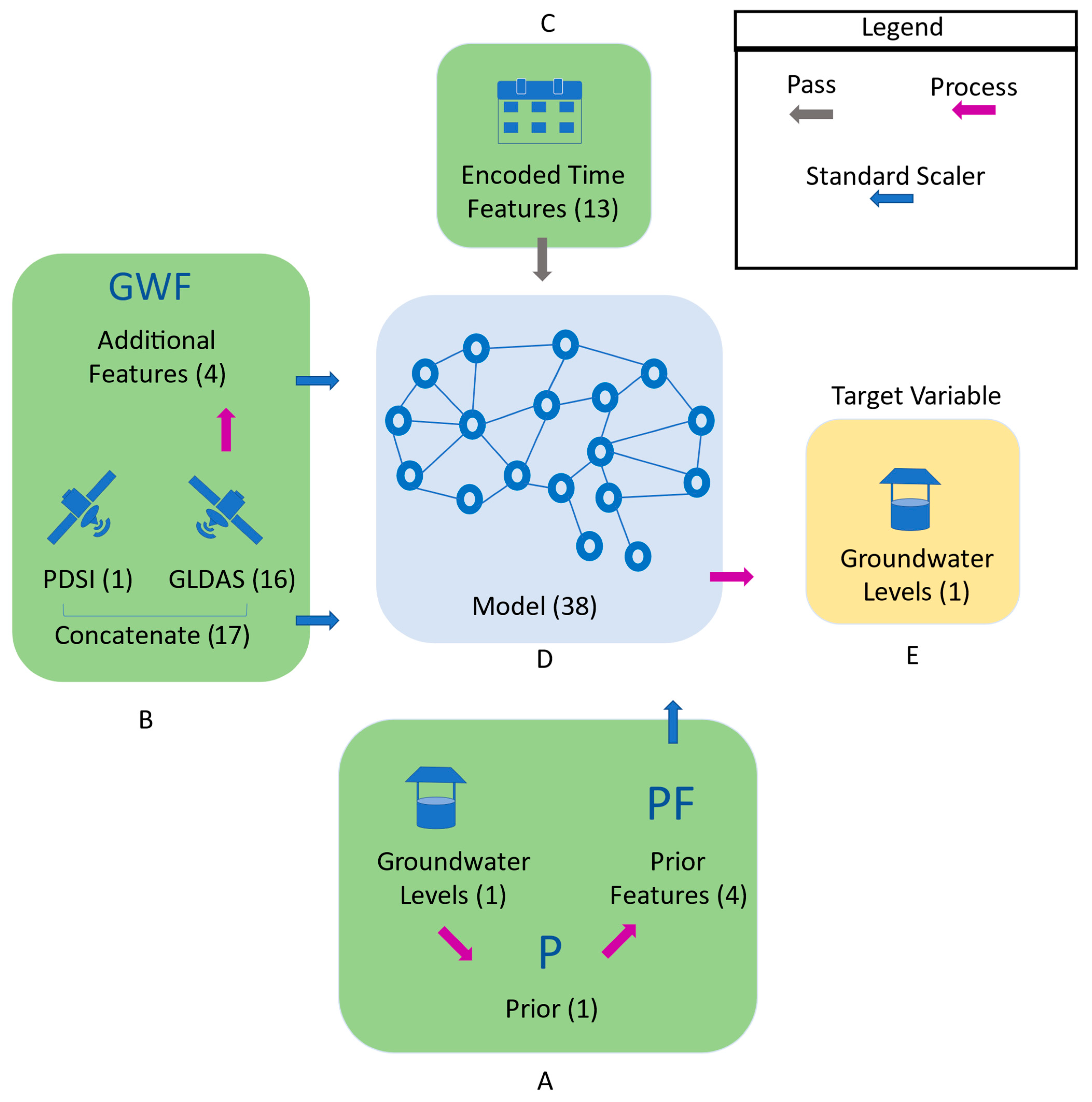
The groundwater imputation workflow is illustrated graphically in Figure 1. To select the target dataset for each well, we reviewed the observed groundwater-level data to ensure sufficient observations exist and remove outliers. We then interpolated these data by using PCHIP to estimate values at the start of each month, so the groundwater data are synchronous with PDSI and GLDAS values. We only used PCHIP to estimate first-of-the-month values if there was a measured data point within 120 days of the first of the month. This means that we used PCHIP to interpolate over small gaps of less than three months. We used these monthly groundwater-level data as the target variable.

We generated prior estimates of groundwater behavior by using these data (details in Section 3.4.2). This prior represents potential estimated trends or structures based on the observed data. We generated an initial prior based on trends. We then used a smoothing algorithm to generate 4 priors that were used as independent features in the regression model, which captured trends from the groundwater data; these features were used as input for the regression models (Figure 1A and Section 3.4.2).

We extracted the GLDAS and PDSI time-series data from the cell with the centroid closest to the target well. That is, for each well in an aquifer, we used the Earth-observation-derived data from the cell centroid nearest to the well being analyzed to create the imputation model for that well (Figure 1B). From the GLDAS dataset, we used 16 variables: pressure, wind speed, specific humidity, sensible heat net flux, baseflow-groundwater runoff, potential evaporation rate, temperature, total precipitation rate, soil moisture (0–10 cm), soil moisture (10–40 cm), soil moisture (40–100 cm), soil moisture (100–200 cm), plant-canopy surface water, snow-depth water equivalent, net long-wave radiation flux, and net short-wave radiation flux. Using the GLDAS data, we generated four engineered groundwater features, namely SW, LnGW, LnPS, and SM, which are presented in more detail in Section 3.2.

We one-hot encoded the month of the measurement and transformed the time (i.e., date) of the measurement to the decimal time set between 0 and 1 over the imputation window. The one-hot-encoded months and decimal time are regression-model features (Figure 1C). Additional details are presented in Section 3.3.

We scaled all the feature data, except for the one-hot-encoded months and the decimal time by using a standard scaler (Z-score transform) based on the statistics of the training data. The standard scaler normalizes the range of the data as deviations from the mean, so all features are on a similar scale. We did not scale the encoded features, because the decimal time is already normalized to the 0–1 range, and the one-hot encoding generates binary features. We trained an MLP model on the target data and independent features (Figure 1D) to create a regression model for data imputation. This resulted in a model with 38 features: 17 from earth observations, 4 derived from earth observations, 13 encoded or scaled temporal features, and 4 prior features. We fitted these 38 features to the measured and cleaned target groundwater-level data to create a regression model that can be used to impute missing data. We repeated the process for each well.

The resulting regression model uses independent data or features that are complete from 1948 to 2020, so we can use this regression model to impute any missing groundwater-level observations within the imputation window (Figure 1E). We want to highlight again that we created a separate model for each well in the aquifer, and we did not attempt to fit an aquifer-wide or regional model.

3.2. Engineered and Derived Features

In addition to the GLDAS data, we derived four groundwater variables that were useful in groundwater imputation: SW, LnGW, LnPS, and SM. The surface-water component (SW) of the GLDAS was an aggregation of six monthly averaged GLDAS variables: soil moisture (0–10 cm), soil moisture (10–40 cm), soil moisture (40–100 cm), soil moisture (100–200 cm), snow water equivalent, and canopy storage [41]. The GLDAS SW component has shown moderate-to-strong linear correlations with the groundwater levels observed in wells [42] and is commonly used in conjunction with the NASA Gravity Recovery and Climate Experiment (GRACE) data to derive groundwater-storage-change estimates [43]. GRACE uses a pair of twin satellites in synchronous orbit to measure anomalies in Earth’s gravitational field to determine how water availability has changed over an area [43,44,45]. We found that SW shows a positive correlation with many of the wells we examined. We added SW as a derived feature because it is based on GLDAS, which is already being used, and provides additional insight into groundwater needs and recharge.

Log-groundwater (LGW) is the natural log transformation of the GLDAS baseflow-groundwater runoff value. We found that this transformation seemed correlated with groundwater use. The 4-month precipitation sum (LnPS) is the rolling sum of natural log of the GLDAS seasonal precipitation value used as an index for recent recharge. LnPS was used to generate context about how “wet” it has been recently. Soil Moisture (SM) is similar to SW but does not include canopy storage or snow water equivalent.

3.3. Encoding Monthly Data and Time Data

For independent values to help incorporate temporal correlations, we established the imputation window (i.e., time period over which we impute data), which is based on the range of the observational data and the meteorological data at a well (or in an aquifer). For our case study, we started on 1 January 1948, as this is the first date with both PDSI and GLDAS data, and ended on 1 December 2020, when the current PDSI extension ends.

We used binary encoding for the monthly time variable to provide temporal information on annual periodicity to the model. This resulted in twelve features, one for each month, in which the value is either a 0 or a 1, depending on the month;

Table 1. Example of the time features; this includes one-hot encoding of the monthly data (green and yellow squares) and the linear time feature in the right-most column.

	Jan	Feb	Mar	Apr	May	Jun	Jul	Aug	Sep	Oct	Nov	Dec	Decimal Yr
1/1/1948	1	0	0	0	0	0	0	0	0	0	0	0	0.0000
2/1/1948	0	1	0	0	0	0	0	0	0	0	0	0	0.0012
3/1/1948	0	0	1	0	0	0	0	0	0	0	0	0	0.0023
4/1/1948	0	0	0	1	0	0	0	0	0	0	0	0	0.0035
5/1/1948	0	0	0	0	1	0	0	0	0	0	0	0	0.0046
6/1/1948	0	0	0	0	0	1	0	0	0	0	0	0	0.0058
7/1/2020	0	0	0	0	0	0	1	0	0	0	0	0	0.9942
8/1/2020	0	0	0	0	0	0	0	1	0	0	0	0	0.9954
9/1/2020	0	0	0	0	0	0	0	0	1	0	0	0	0.9965
10/1/2020	0	0	0	0	0	0	0	0	0	1	0	0	0.9977
11/1/2020	0	0	0	0	0	0	0	0	0	0	1	0	0.9988
12/1/2020	0	0	0	0	0	0	0	0	0	0	0	1	1.0000

shows an example of the encoding. These 12 monthly features allow the model to compute correlations between the groundwater-level observations and the time of year in months, thus capturing annual periodicity. In Table 1, each row represents a measurement date with 12 monthly features, all of which are zero, except for the month of the observation. These features capture processes such as seasonal or annual periodic variations [46]. For example, if the data exhibit an annual periodicity, March levels may be consistently higher than September levels. We created another time feature to correlate with long-term trends or behaviors. This feature is the decimal time since the start of the imputation period, ranging from 0 at the beginning of the imputation window to 1 at the end of the study period. The decimal time variable allows the model to have a sense of order and capture correlations with a linear long-term trend if one exists. In Table 1, the decimal time feature is shown in the right column, it starts at 0 at the beginning of the imputation window (1/1/1948) and then increments by 0.0012 for each month, ending with a value of 1 at the end of the imputation window (12/1/2020).

3.4. Groundwater Priors to Characterize Long-Term Trends

3.4.1. Inductive Bias: The Need for a Prior

Before explaining the methods used to develop the prior, we present a thought experiment to explain why inductive bias (estimated prior behavior) helps obtain better groundwater imputation results and how adding this additional information can assist time-series imputation over long gaps. In a typical machine-learning problem where a time series is being regressed on feature data, we obtain observational data and select feature data. Next, we develop a hypothesis (or model) to regress the feature data on the observed data. Then we use the resulting model to impute any missing data. We assess how well the model generalizes on novel instances by reserving a test dataset and calculating error metrics to determine if the resulting model predicts the right output and check if we “overfit” the model. A model that is overfit has significantly higher errors on the testing data than on the training data. If the training and testing error metrics are similar, the model is not overfit; in other words, the model can be used to estimate or impute missing data.

However, for our problem, groundwater imputation, a problem arises when all the observational data are from a small portion of the study period that does not capture significant long-term trends or other apparent structure in the data. In these cases, we use induction bias or prior estimates of groundwater behavior to make assumptions about the general behavior of the data; for example, are they periodic, are they linear with a trend, or do they follow some other structure? In most regression problems, the data are independent, and we assume that the sample data represent the larger population. For time series regression, where we treat the data as independent, but they actually have time-correlation features, the data can have a unique data shape or data structure that represents the general trends and processes over time. We can estimate these long-term trends from the existing data if these data exhibit some of these same trends or structures. By creating prior estimates of long-term behavior on existing data, these data can be used to help estimate the missing values. To successfully regress time-series data, the selected features need to describe the time-varying behavior of the target variable, and we need sufficient observations so the algorithm can properly determine the general structure of the data and its correlation to the inputs.

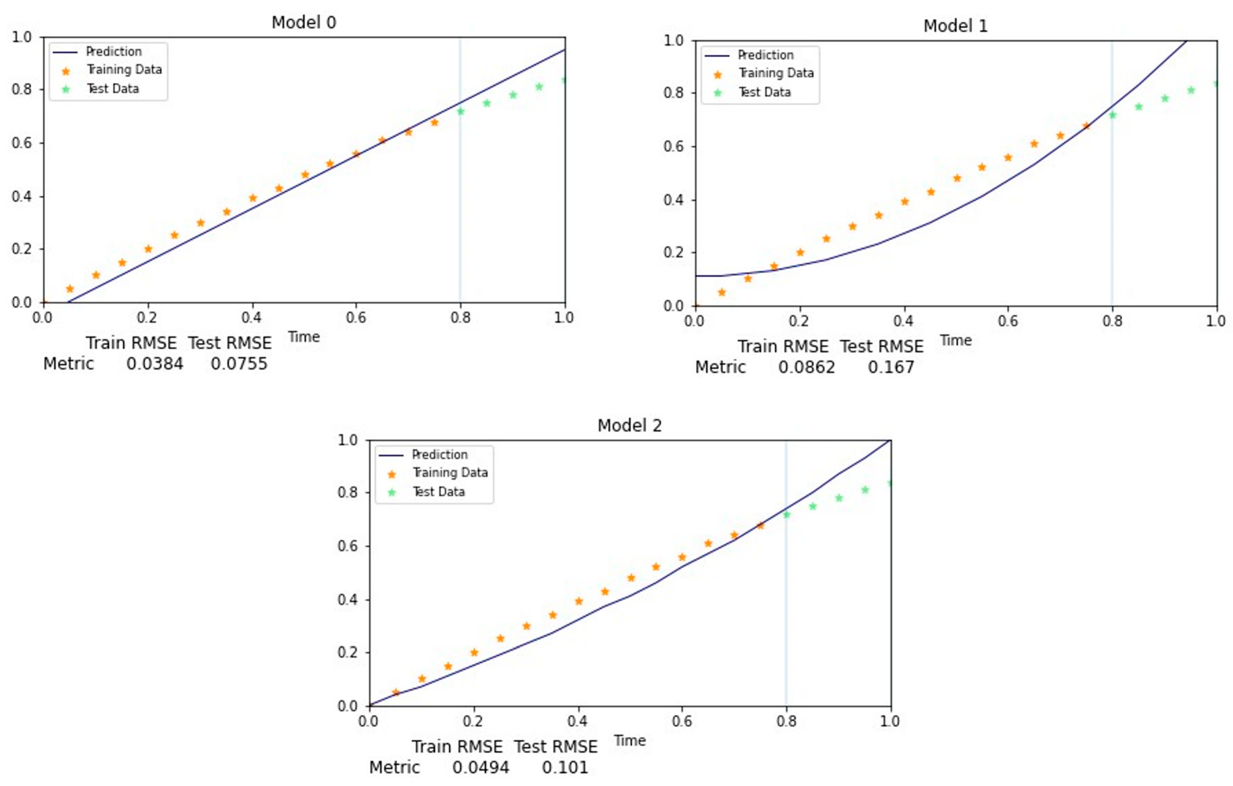
We present an example in Figure 2 wherein we built a generic model with an 80–20 training–testing split, with the training data shown in yellow and the testing data shown in green. These data represent a short period from a longer dataset. The error metrics for each model are shown. We selected three basic model forms: linear, quadratic, and a power law. All three models perform reasonably well on the training data but struggle to generalize on the test set. Based on these plots and error metrics, there is no strong indication that any of the models are overfit, and it is not clear which model is best. Based on the error metrics alone, Model 0 performs best on the test data, and without other information, it would be selected as the best model to impute the rest of the data in the imputation window.

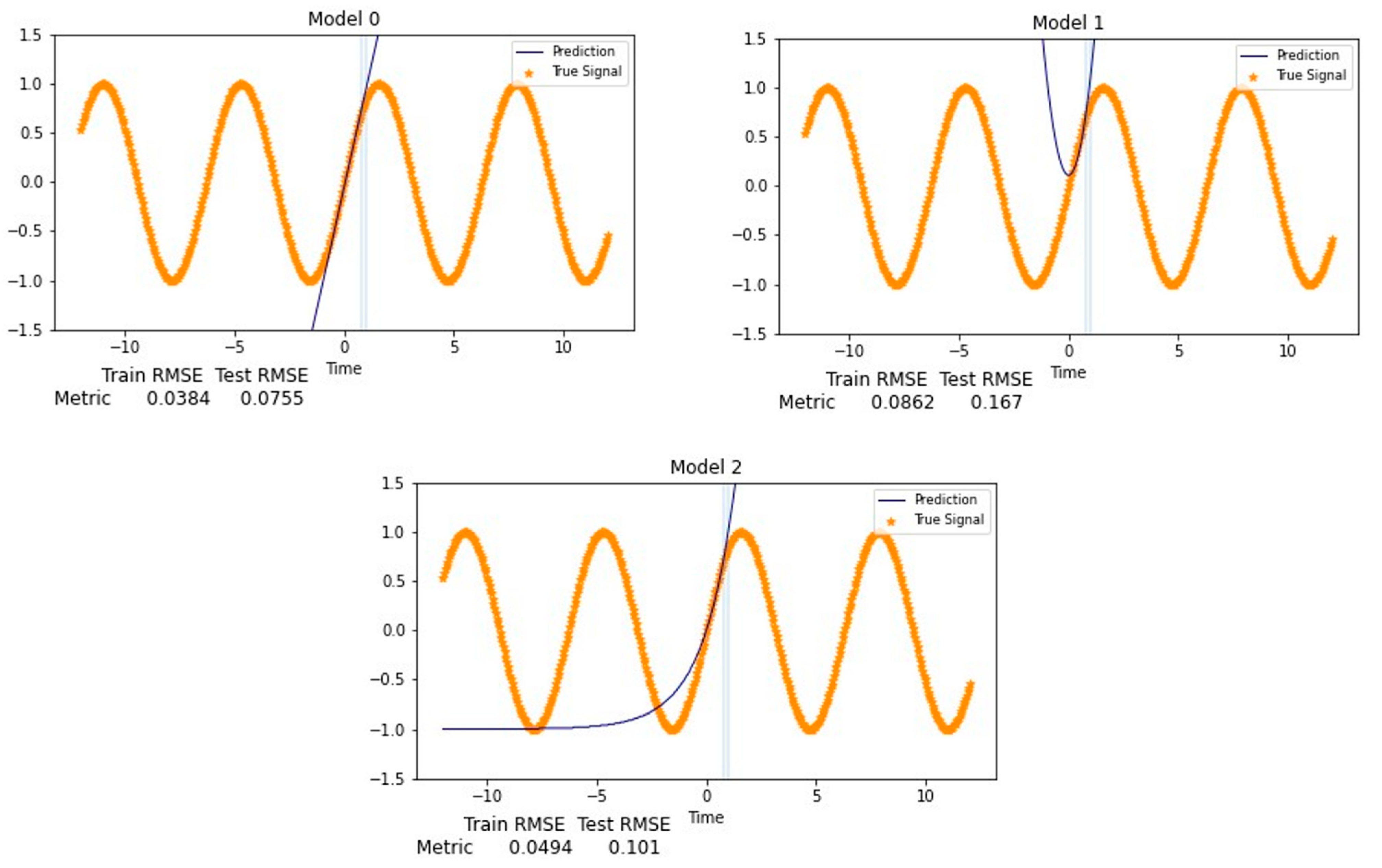
Figure 3 shows how the models from Figure 2 would generalize on the true long-term signal if it were possible to obtain more observations. In this example, the actual data are sinusoidal, but the observation data come only from a small segment on a rising limb. As expected, all the models generalize poorly, and any imputation performed by these models would not be useful over a longer imputation window. By “generalize poorly”, we mean that the model does not produce values that behave as typical groundwater measurements. The reason is because there was not enough information in the training set to properly determine the structure of the data to predict missing values; this is known as an ill-posed problem. This issue has nothing to do with the model’s overfitting and everything to do with not having enough representative data.

During groundwater imputation, we often experience a similar situation as mentioned above, where we build a model based on the sparse observations available, but the model predictions may not represent the actual groundwater change because the model does not have enough context about the situation, and it is impossible to know the true signal. If data are missing over long time periods, the general trends and structure, such as annual periodicity, are not captured by the regression equation. As a result, when a well has sparse observations, there are an infinite number of models that appear to give good results based on the training and testing metrics but generalize poorly when used out-of-sample.

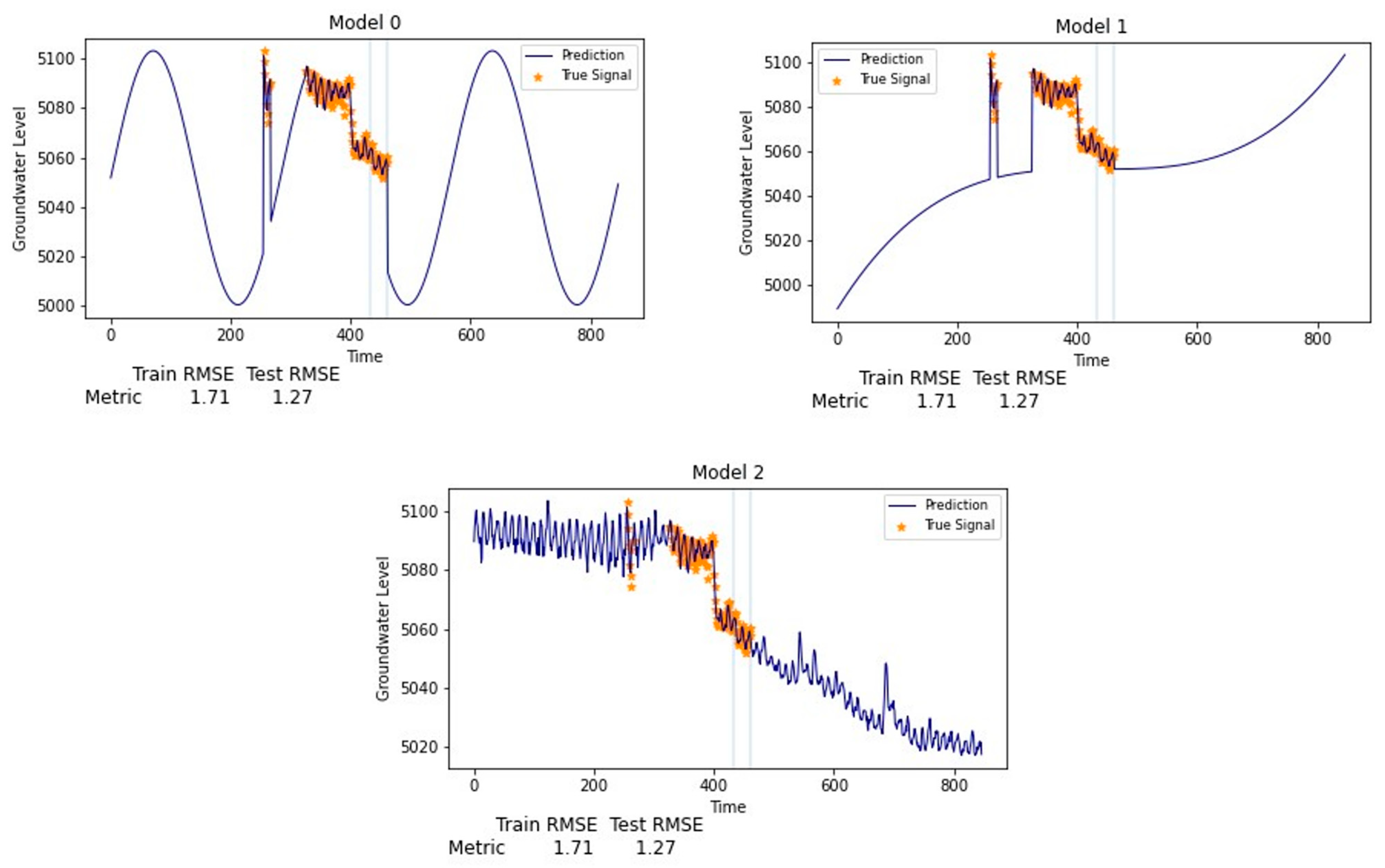
Figure 4 presents three models for imputing groundwater data from an actual aquifer assuming different model forms or hypotheses. The observed dataset has dense observations in the middle of the time period, with large gaps on either end. Even though the data over these large gaps are estimated by regression, rather than extrapolation, the models make different assumptions about the data out-of-sample, and the resulting imputed data are very different. By all metrics on the available data, all three models are the same; that is, the error metrics on both training and testing data are the same. However, each model makes different assumptions about the general trends, periodicity, and structure of the missing data. For these situations, we can use inductive bias or prior information to prefer one model hypothesis over others based on how well it resembles our understanding of groundwater hydraulics and behavior in this aquifer. A trained hydrogeologist knows that the groundwater should generally have a declining trend in an aquifer under overuse, and these data should have a seasonal element representing recharge and pumping loads. Most hydrogeologists, or people familiar with groundwater behavior, would prefer Model 2 from Figure 4 over the other two models to represent imputed groundwater behavior, even though the error metrics on all available data are identical. The reason for this is because we have a preconceived or prior idea of how groundwater behaves and background information on local trends. If we were to inform our models with this information, we could add a domain-specific bias to constrain our model space and obtain better generalized results based on our domain knowledge of groundwater.

In summary, we added bias by using prior estimates of groundwater behavior to make the model prefer a hypothesis which has the structure which represents expected groundwater behavior. To accomplish this, we developed an initial prior estimate of the missing data and generated prior features to use in our model. These features inform our model on a data structure that better matches our preconceived insights of how the gaps in the data should be filled based on in situ data, while the meteorological data inform the model on the seasonal variance and measured climatic and environmental trends.

3.4.2. Developing a Generic Prior and Prior Features

Developing a general method to create a prior by using only data without direct involvement and that works well is challenging. We created a prior that is a data-centric estimate of the long-term trends for a well based on the available in situ data for that well. We used these data to estimate long-term trends. However, when estimating long-term trends, very different results occur depending on which data are used to estimate or extrapolate the trend. These extrapolated trends depend on the size of the window analyzed or which data points were used or exist.

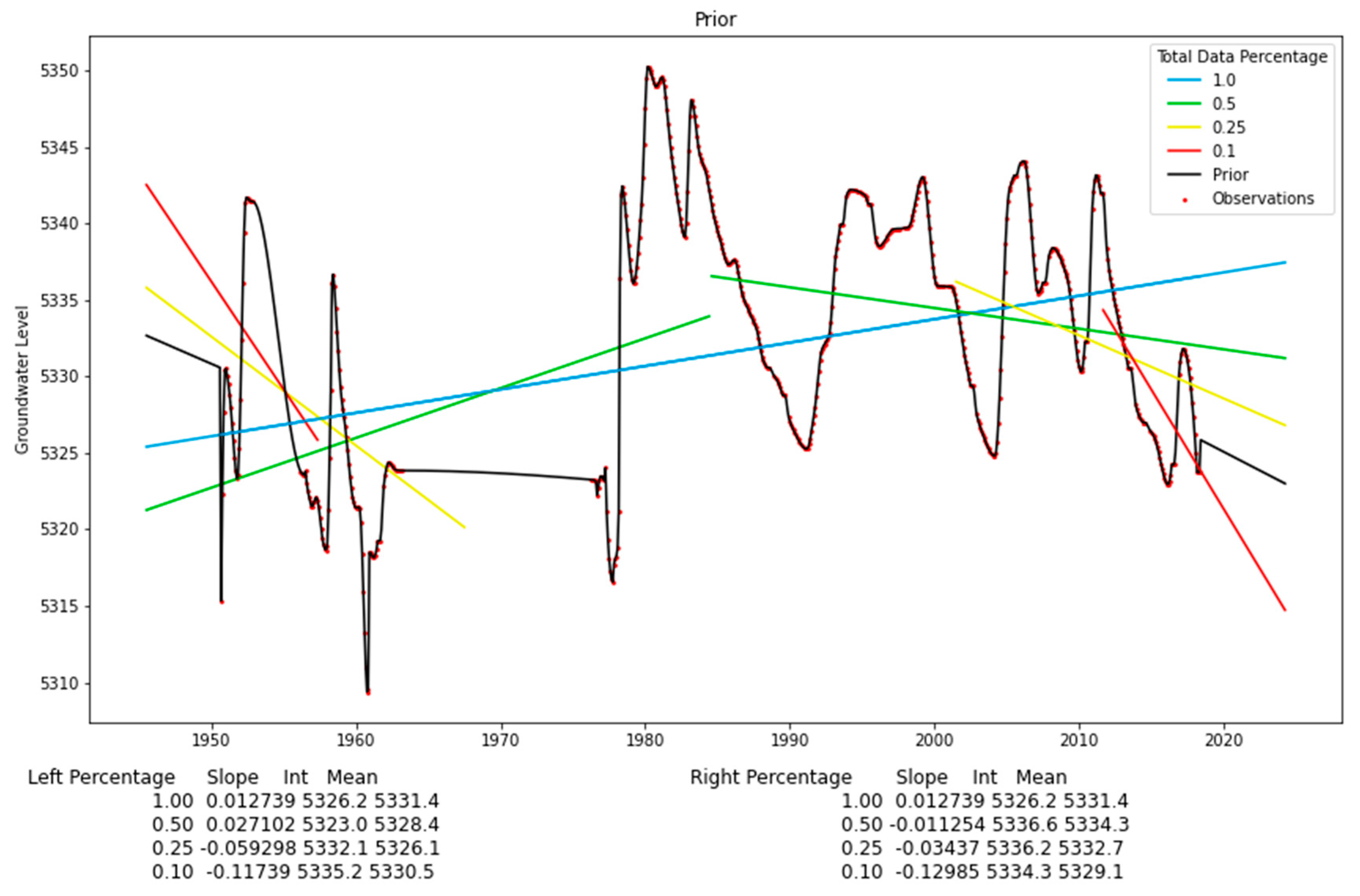
We generated our prior as a piecewise function composed of three sections: interpolation, extrapolation, and limits. Within the temporal range of the data, we generated the prior by interpolating the observed data, using PCHIP. Because we have observed data, it is easy to see the trend between individual measurements. This is shown in Figure 5 as the black line inside the range of the data.

Next, we wanted to capture the apparent trend outside the range of the data. To do this, we computed 4 linear regressions for each side of the data, using 10%, 25%, 50%, and 100% of the data, respectively. During these regressions, we removed outliers from the subset. These estimates are shown as the red, yellow, green, and blue lines for the trends based on 10%, 25%, 50%, and 100% of the data, respectively. To generate the remainder of the prior (the region outside the limits of the data), we averaged the slopes of the four linear regressions and extrapolated the data to the limits of the imputation window, using this average slope and the mean of the 10% subset of data on the respective end as the intercept. Figure 5 shows an example prior (black line), which we generated by using PCHIP interpolation which honors the data limits. The extrapolation covers the entire study period from July 1945 to June 2023. Notice that the black line follows regions with existing data closely, generates smooth curves over data gaps (e.g., 1955–1958), and extrapolates a weighted average trend outside the limits of the data (e.g., <1950 or >2020).

We used this prior to help capture the structure and trends present in the data. This prior is not an accurate estimate of the missing data and is quite dependent on where the dataset ends. We found, however, that this prior, and the resulting features, greatly increased the accuracy of our imputation models. In Figure 5, for example, we see that the trend estimated by the last 10%, 25%, or 50% of the data shows that the groundwater-level trend is decreasing rather quickly. However, the trend computed from 100% of the data shows a positive slope. Our prior averages these competing slopes so that the extrapolation data in our prior do not change as quickly. As a result, this prior estimate of the entire dataset captures information from the existing data and provides information on long-term trends.

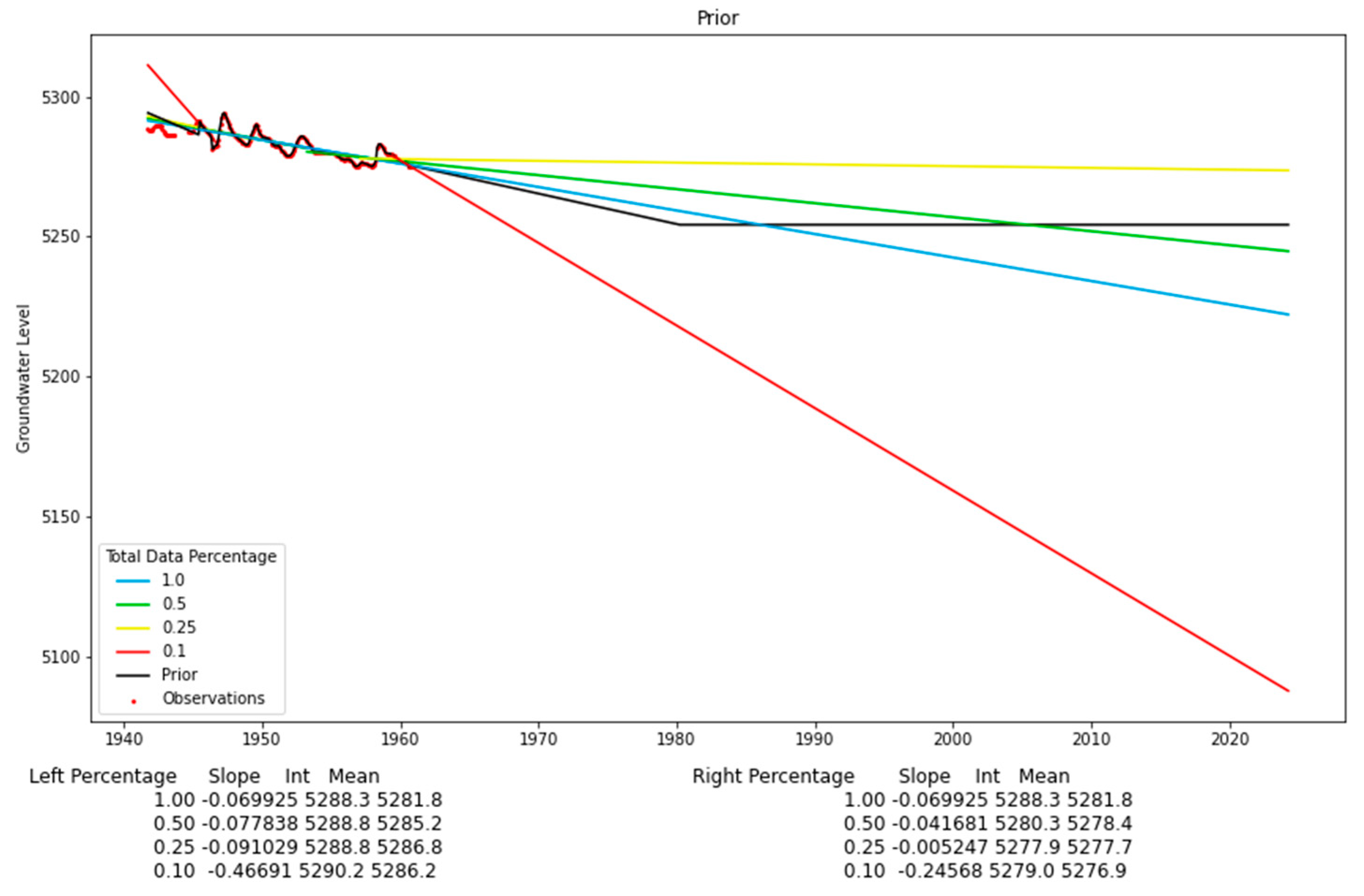
The “limit” is a ceiling or floor on the data that works as a data quality check on our extrapolation. We limit the extrapolated data to 6 standard deviations above or below the mean of the observations. We added this limit for situations where either the average slope used for extrapolation was large or the extrapolation period was long. In these cases, extrapolating the data results in values that are physically unlikely. Figure 6 shows an example from a different well with data near the beginning of the study period. The prior for this well requires extrapolating the data over a long time period, from about 1960 to 2020. Figure 6 presents the trends estimated by using 10%, 25%, 50%, and 100% and the prior (black line) generated by using the weighted average of the trends and an imposed limit. This figure shows how the extrapolation using the trend from 10% of the data results in unrealistic values. In this example, the prior reaches the limit during 1980, with the value remaining constant over the remainder of the extrapolation. We selected 6 standard deviations empirically by analyzing the range of different wells and determining how large of a change could be expected over the ~70-year study period.

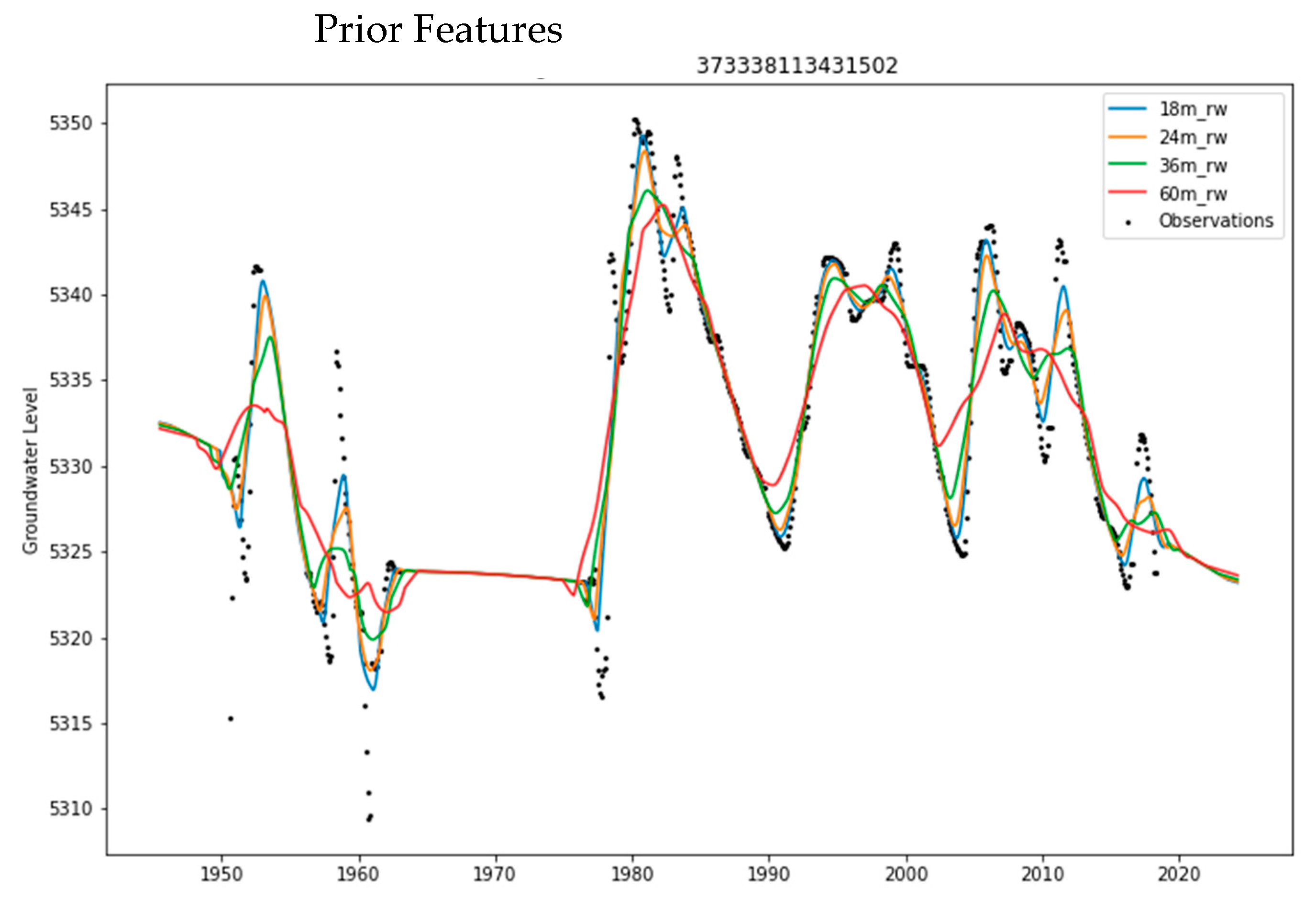
To extract the four prior features, we use as model input from the initial prior; we use a centered moving window with four different sizes, namely 18, 24, 36, and 60 months, to smooth the initial prior. This approach requires that the prior has an additional 30 months (half of the largest window) of data before and after the imputation window in order for the center rolling window to have the same temporal range as the GLDAS and PDSI features (1948–2020). To act as features for the regression model, these features must be a complete datasets; that is, they need to have values for every point in the imputation window. To meet this constraint, we extend the extrapolation to these limits. These four trend features provide the model with an initial estimate of general groundwater-level trends and temporal corrections. Figure 7 shows the resulting four trend features computed for the prior shown in Figure 5.

The prior features are a smoothed version of the groundwater observations and the estimated prior. Each feature captures different information regarding groundwater-level inflection points depending on the size of the rolling window. During training, the model is only fit in regions were groundwater-level data exist. The use of multiple prior trends—four in this case—helps the model to not cling onto a single feature with high correlation.

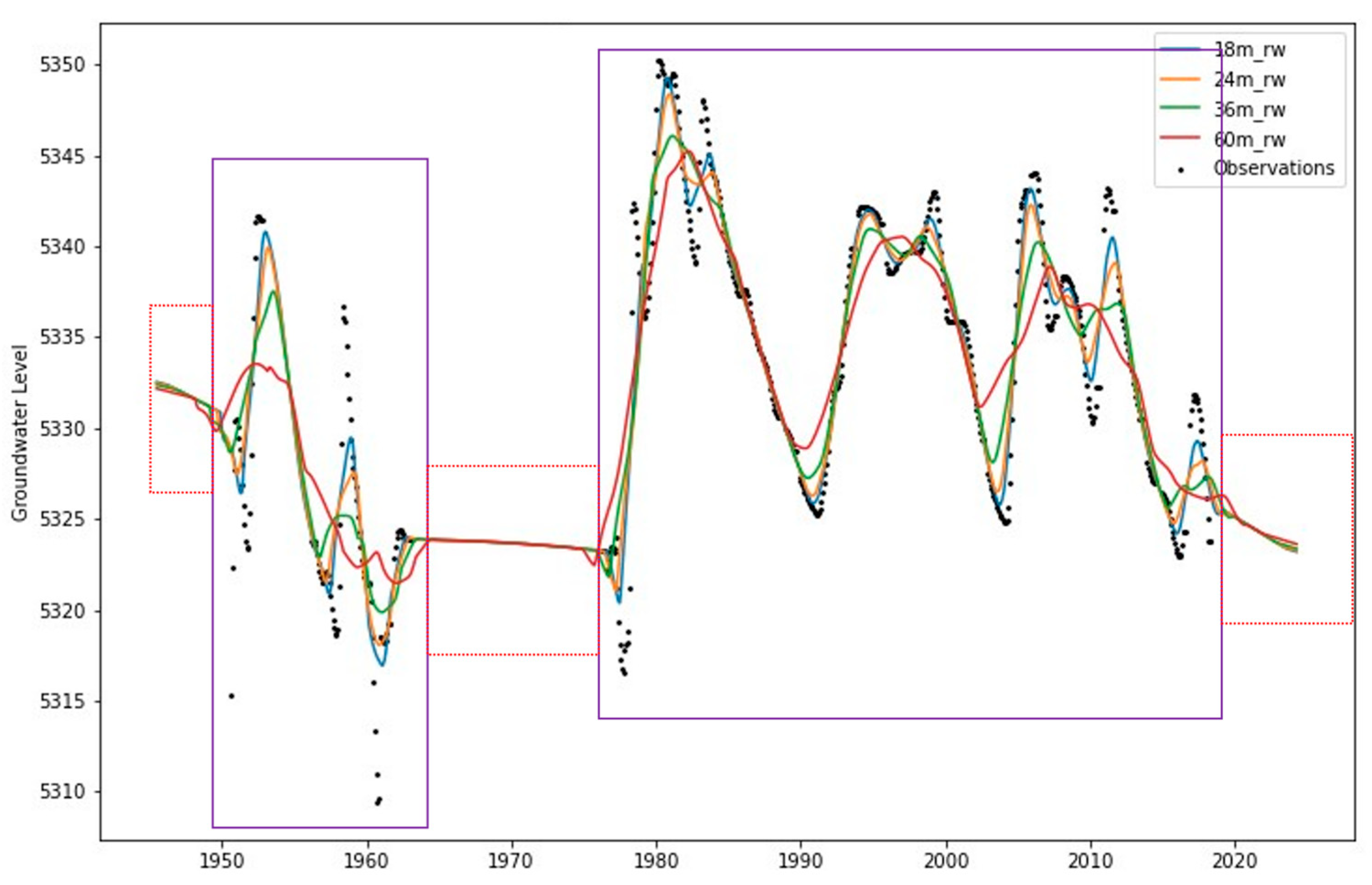
Figure 8 shows regions where there are no observation data as red boxes. The trend features in these regions do not affect the fit of the model, as there are no data to train on. The model will fit the trend features, along with the other 34 features, to the observation data in the regions shown by the blue boxes. The resulting correlations will influence imputation results in the regions defined by the red boxes, adding information about trends and structure in the data. The prior features act as an initial approximation (i.e., a prior) of the groundwater-level data. The prior features provide the general trends or shape we would expect the well data to follow, while climate data provide the seasonal variation.

3.5. Machine-Learning Modeling

Though our ultimate research goal was to analyze long-term storage trends in an aquifer, we found that we could impute missing data most accurately if we developed an individual model for each well in the aquifer, rather than a single model for the aquifer as a whole. We used these models to impute missing values for the well within an imputation window from 1948 to 2020. This provides a complete dataset for each well that can be used to analyze the long-term storage in the aquifer.

We used an MLP model architecture with two hidden layers of width 50 and 100 nodes for the 1st and 2nd layers, respectively. We applied L2 regularization and 20% dropout between layers to prevent overfitting. Regularization limits the impact of features used in the model, as this is important in cases such as ours, where the number of features and the number of data are similar. We fit the model by using the Adaptive Moment (Adam) optimizer [47].

The model matrix has 38 independent features consisting of 16 GLDAS variables, 1 PDSI variable, 4 prior features, 13 temporal features, and 4 derived variables. In most machine-learning problems, the number of observations (o) is much greater than the number of features or predictors (p): o ≫ p. In our case, o ≅ p. If we used a traditional train/test split, this would result in datasets for many wells, where o < p. Because of this, we used K-fold cross-validation with 5 folds to estimate the error, and then we used the entire dataset to fit the final model as a means to involve all of our data in the training. K-fold cross-validation determines the accuracy of the model, or model error, by stochastically creating models with different selected training and testing data [46]. K-fold splits the data into five groups containing a similar number of sequential observations where each model uses a different test set. For each fold, four groups are used for training, and one is used for testing. We compute and average the error metrics for each fold. We train the final model by using all available data. We use the average number of epochs determined during K-fold validation to train the final model to mitigate overfitting. We then use the average values from the individual folds to estimate error metrics.

This approach allows us to create useable models with a minimum of 50 observations, while still evaluating overfitting and providing error metrics; however, more observations would produce better results. At the lower limit of 50 observations, if we built a single model by using a typical 80–20 split with a 30% validation set for early stopping, 10 points would be set apart for testing, and 12 points would be set apart for validation. For a well with only 50 observations, we have only 28 observations for training with 38 features. It is difficult to address overfitting in this case, as you can exactly fit a linear model; that is, the error would be zero. You can use various regularization methods to reduce the number of features, but it is still difficult to estimate error and generalization. K-folds help address both of these issues. Another benefit of using K-fold to validate our models is that the final models use all the available data, thus generating better models.

We developed the models by using the Python programing language with the Keras and TensorFlow packages [48,49]. Keras and TensorFlow are high-level frameworks that facilitate the implementation of machine-learning models and make it easy to explore different model architectures and parameters.

4. Case Study, Results, and Discussion

4.1. Case-Study Location

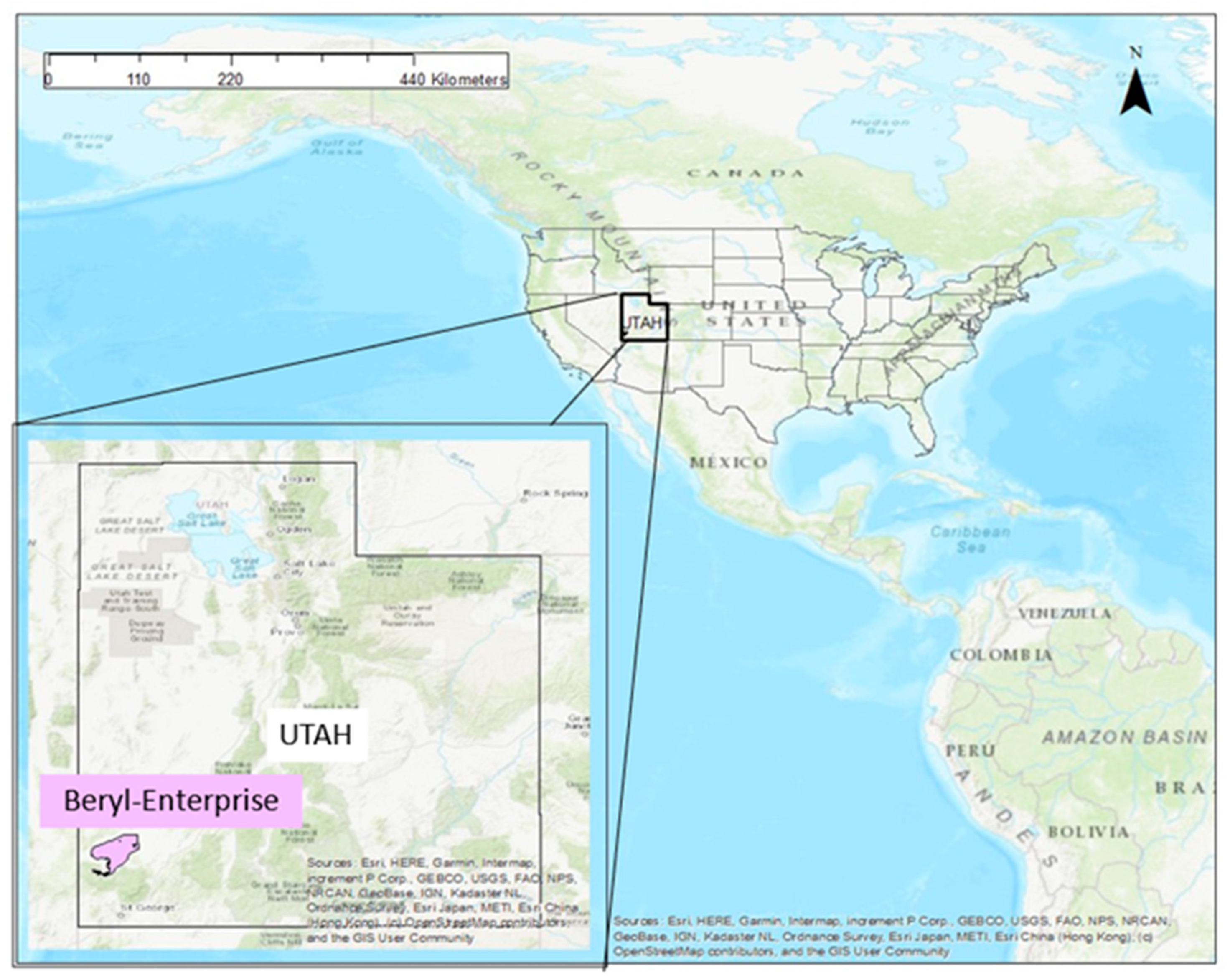
To demonstrate our approach, we used historical water-level data from the Beryl-Enterprise aquifer in Utah’s Escalante Desert. We chose Beryl-Enterprise because many of the wells in the aquifer have rich observational records, with some extending back to 1935. The Beryl-Enterprise aquifer is part of the Great Basin aquifer located in the Beaver River drainage basin. The aquifer has an area of approximately 433 square miles (1121.4 sq. km) and is located 40 miles (64.3 km) west of Cedar City, Utah (Figure 9). The valley which contains the aquifer is almost surrounded by mountains and varies in elevation between 5500 and 8500 feet (1676.4 to 2590.8 m). The aquifer is underlain by consolidated rocks ranging from the Cambrian to Tertiary ages and unconsolidated and semi-consolidated rocks from the Quaternary age [50]. The top 500 feet (152.4 m) consists of coarse-grained deposits, mostly sand and gravel. A clay and silt deposit that somewhat restricts vertical water movement exists between 500 and 1000 feet (152.4–304.8 m) of depth. The saturated thickness of the aquifer is approximately 1000 feet (304.8 m).

Until the 1920s, groundwater withdrawal was primarily for domestic purposes, and then the need shifted to agricultural irrigation. Water levels in the region have trended downward since 1940. Groundwater withdrawal in the area increased from 3000 acre-feet (3,700,000 m³) per year in 1937 to 80,000 acre-feet (9,900,000 m³) per year in 1977. In 1977, recharge to the groundwater reservoir was estimated to be 48,000 acre-feet (59,207,040 m³), resulting in an approximate 30,000 acre-feet (37,004,400 m³) per year deficit [50].

4.2. In Situ Data Preparation

We obtained groundwater-level observations for all wells in the aquifer. For the 751 wells in the area, only 57 of these wells had at least 50 unique observations over the imputation window of January 1948 to December 2020. The well observations are sparse and are sampled monthly, quarterly, semi-annually, annually, or less frequently depending on the well. Water levels in the area reach an annual high in the spring, immediately preceding the new irrigation season, when higher pumping starts, with annual lows typically observed during the fall, at the end of the irrigation season, after which water levels exhibit some rebound during the winter months.

To prepare the groundwater measurements for imputation, we need to first convert the measurements, which are typically depth-to-groundwater, to groundwater levels; we then subtract the depth to water measurements from the elevation of the top of the well. In many areas, especially in developing countries, the ground-surface elevations are not known; in these cases, we interpolate a surface elevation for the well by using a digital elevation model (DEM) such as the Shuttle Radar Topography Mission (SRTM) DEM published by the NASA [51]. For wells in the United States, we typically download wells and historical water levels or depths from the National Water Information System published by the United States Geologic Survey (USGS) [52]. We process the water-level data for outliers by removing observations that are more than three standard deviations from the mean. Next, we use PCHIP to interpolate data to estimate values at the start of each month, so the groundwater data are synchronous with PDSI and GLDAS values.

To continue the data preparation process, we remove wells that do not contain measurements in at least 50 unique months between January 1948 and December 2020, after filtering for outliers. By evaluating the number of unique months, rather than the total number of data points, the data are more likely to represent the general trends at the well. In our experience, it is not unusual for a well to have 50 data points, though often the measurements are only available over a relatively short time period and not spread out through the imputation window. We selected the threshold of data to be 50 unique months, as a general guideline based on our experience with groundwater data and neural networks; our best results occurred from models with at least 150 unique monthly observations over the time period of 1948 to 2020, a period of approximately 874 months. Of course, more representative data reduce the variability and bias in the model, as the relationships between groundwater levels and climate change over time.

As discussed in the overview, we use PCHIP to interpolate values at the start of each month and impute data over small gaps, less than 120 days (4 months). This slightly smooths the data, provides synchronous observations with the GLDAS and PDSI data, and generates additional data for training. We call the 120-day length “padding” and selected this value by using an ad hoc trial-and-error approach. We found that the accuracy of the imputation results over these short gaps is relatively insensitive to padding values from 30 to 120 days. However, a longer padding results in more training data, and these data are helpful, as there is a limited number of observations. Larger paddings may be used; however, this tends to over-smooth the groundwater dataset, and the seasonal fluctuations shown in the meteorological data are lost. We use PCHIP because it honors the data limits but does produce smoothed, less variable data. We found that PCHIP interpolation for data within 120 days of an observed data point was within acceptable limits because groundwater levels change slowly [53]. The 120-day padding generates a maximum of eight months of additional data per gap, as up to 4 months of data can be interpolated from either end of the gap from existing observations. If the gap is at the beginning or end of the dataset, a maximum of 4 months of data can be generated. We repeat the resampling and infilling process for every well in the aquifer prior to fitting the models for each well.

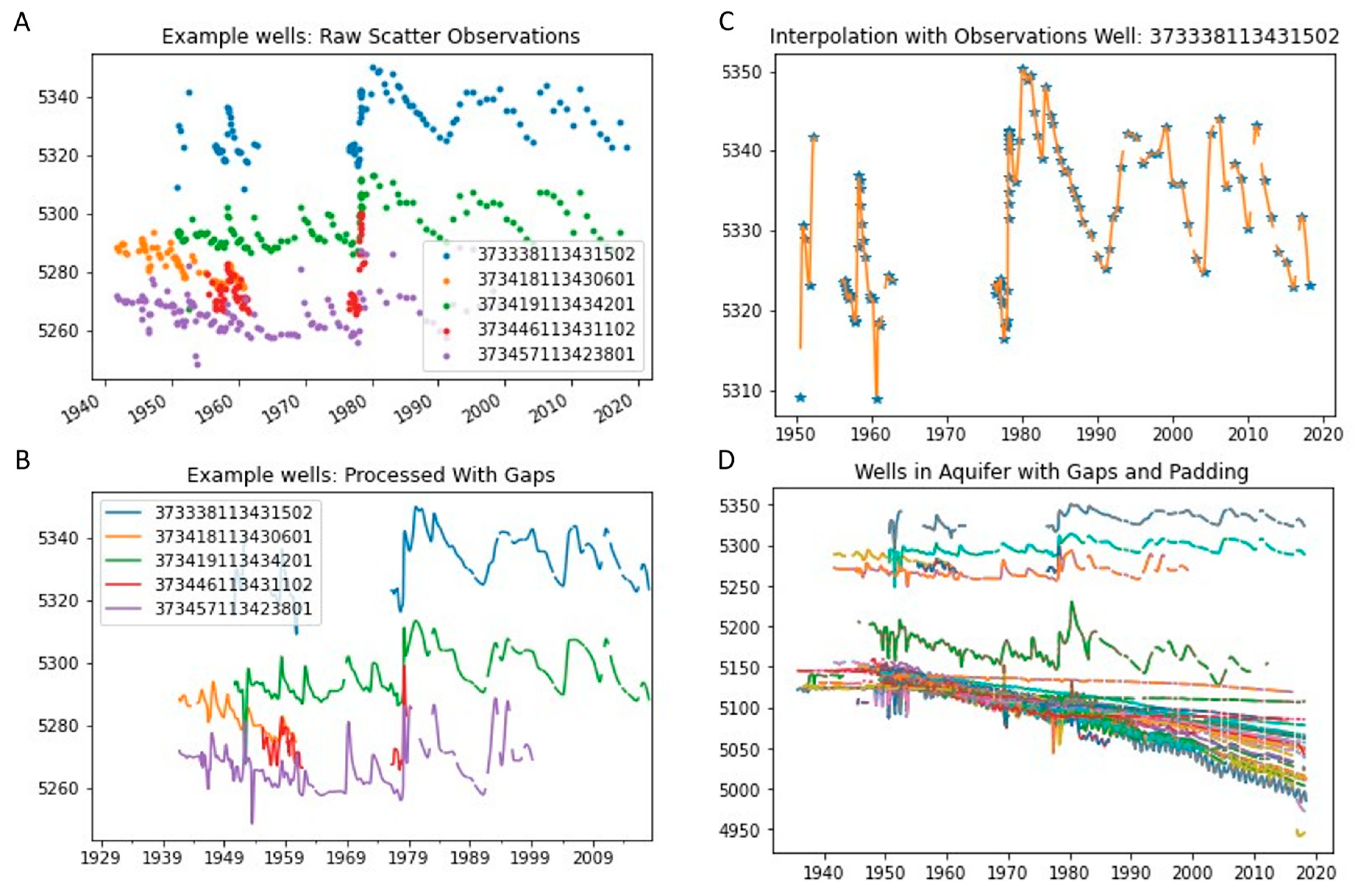
Figure 10 shows an example of this process for the some of the wells within the Beryl-Enterprise aquifer in Southern Utah. The first panel (A) shows the raw observation data for five different wells. The second panel (B) shows the results of applying the PCHIP resampling to the beginning of the month and infilling gaps less than 120 days on the same five wells from panel (A). Panel (C) displays details for a single well, where the blue “stars” are the original data points, and the yellow lines are the data after PCHIP resampling and infilling. This clearly shows the data trends and periodicity at this well. At locations with only a single point, panel (C) shows how the PCHIP-generated data assume that the trend is toward the next data point, even if they are a significant distance away. The last panel (D) shows the results of applying the resampling and infilling processes to all the 57 wells in the aquifer.

4.3. Imputation Results

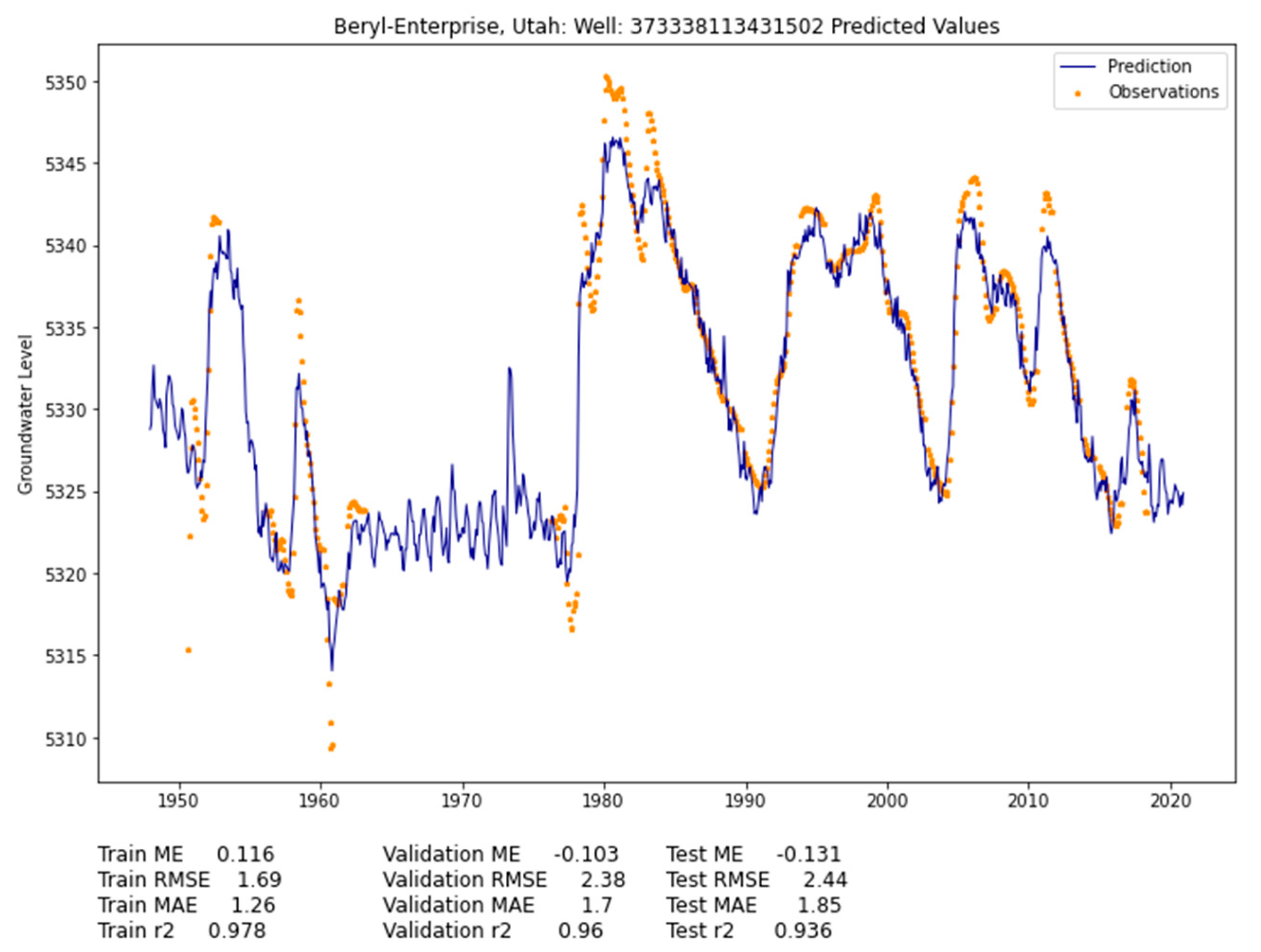
Our approach is a general method and can be scaled and applied to any location in the world if sufficient data exist. We tested the method by using wells and water-level records from the Utah Beryl-Enterprise aquifer described in Section 4.1. Figure 11 shows an imputation example for Well 373338113431502. This is a simple example because there are many observations spread over time. These data provide a good context for long-term trends and other structures in the record. This well has 545 observations within the imputation window with two major gaps: the first is a smaller 4-year gap between October 1952 and March 1956, and the second is a larger 13-year gap between February 1963 and April 1976 (Figure 11). Figure 11 shows both the estimated values, labeled “prediction”, as a blue line, and the measured data, labeled “training data”, as orange points. We included both in Figure 11 to show how well the machine-learning model predicts the observed excursions in the data and closely approximates observed minima. The computed mean error shows that model predictions are slightly biased low with an RMSE of ±2.39 feet (6.2%). Based on the slow-changing nature of groundwater, the values that appear during the gaps seem like reasonable estimations where imputed values continue having seasonal trends that follow meteorological observations while maintaining the overall trend in the data (Figure 11).

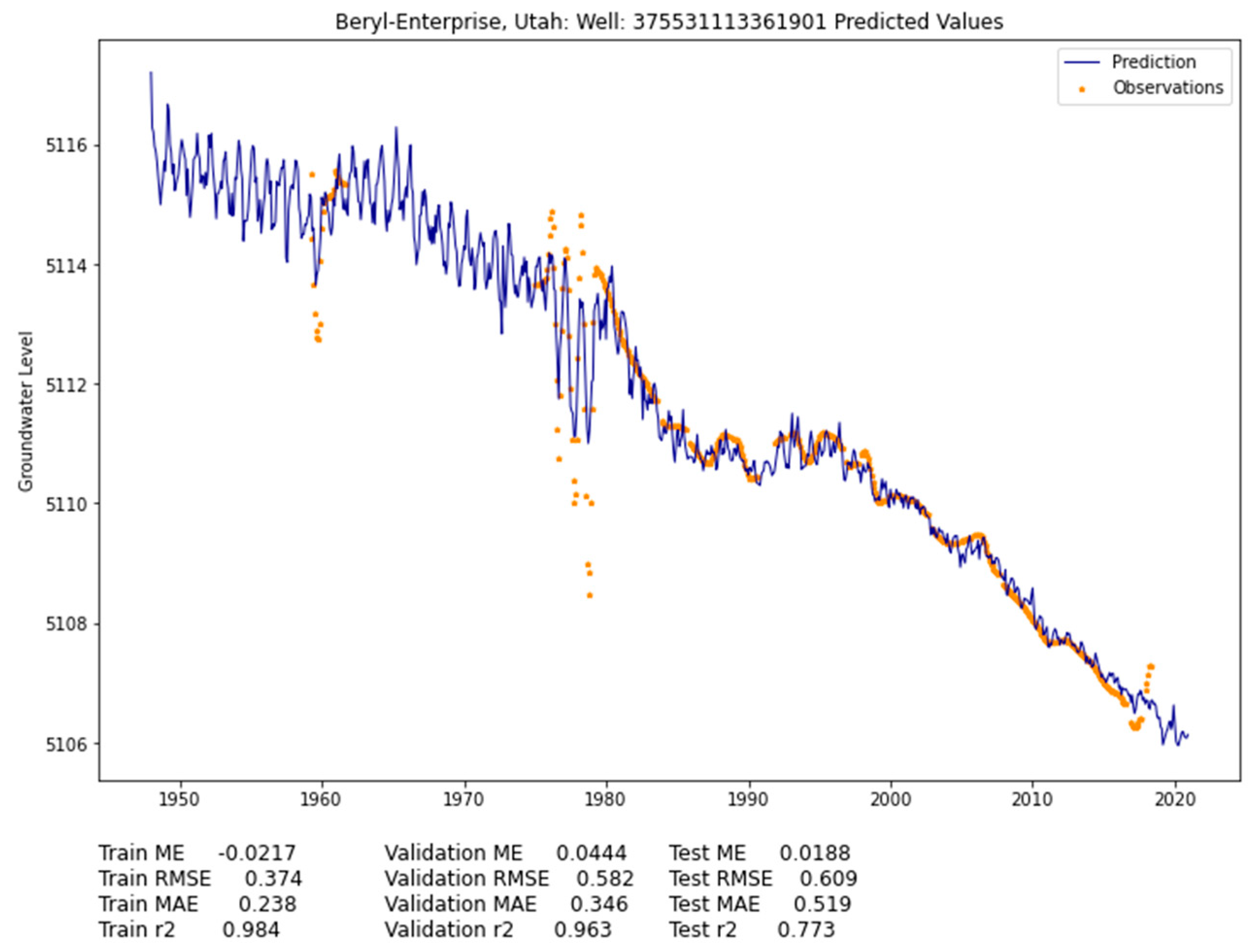
Figure 12 shows an increasingly more difficult well structure to impute. We have most of the observation points from 1973 through 2018, with large gaps from 1948 to 1957 and from 1961 to 1973. The reason why this well is more difficult to model is because we have many rapid changes in the groundwater levels from 1979 to 1980, and from then onward, the well has a rather complex shape. The imputation model performs exceptionally well on this well, having an RMSE of 0.609 (0.05%) and being able to capture a reasonable shape based on the observations.

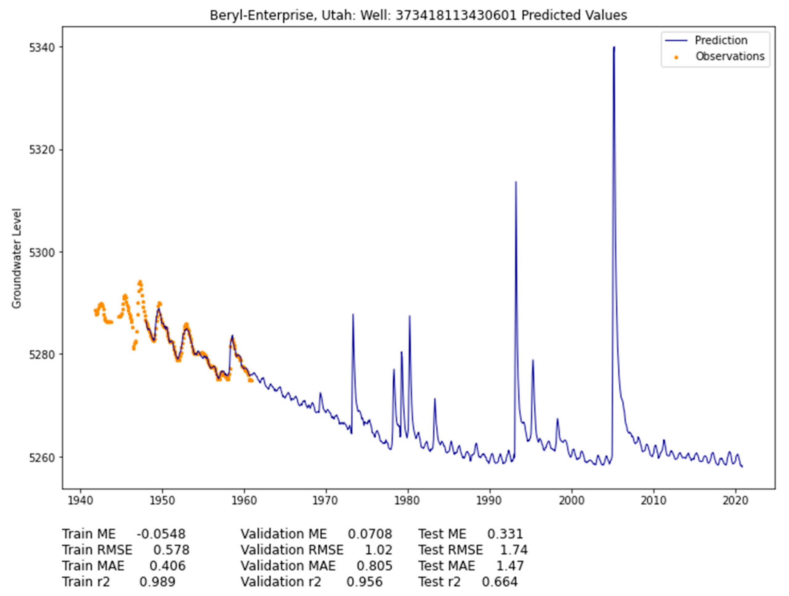
Figure 13 shows a more difficult well to impute. This well has 149 unique monthly observations between 1948 and 1966, with 62 unique months of data before 1948. This well has no data after 1966—a 55-year gap—meaning that the trends and structure in this period must all be inferred from the features provided to the model. This situation relies more on the prior estimates to provide trends and structure to the algorithm. The existing early observations display seasonal periodicity with a significant decreasing trend. The prediction replicates the seasonal periodicity and much of the variation with the downward trend continuing until approximately 1990. The increases in 1982 and 1983 were very wet years, so this matches expectations. However, this model contains large excursions that are unreasonable during 1993, and 2008 for groundwater movement. Although this is a good initial estimate of how groundwater at this well has changed, it could be improved. The general trends and periodicity are consistent with expectations, with the exception of these excursions, which we discuss further in the context of all the wells in the aquifer. This model depicts the challenges of evaluating the models statistically since based on our tests, we have a predictive error of only 1.74 feet (~10.2%).

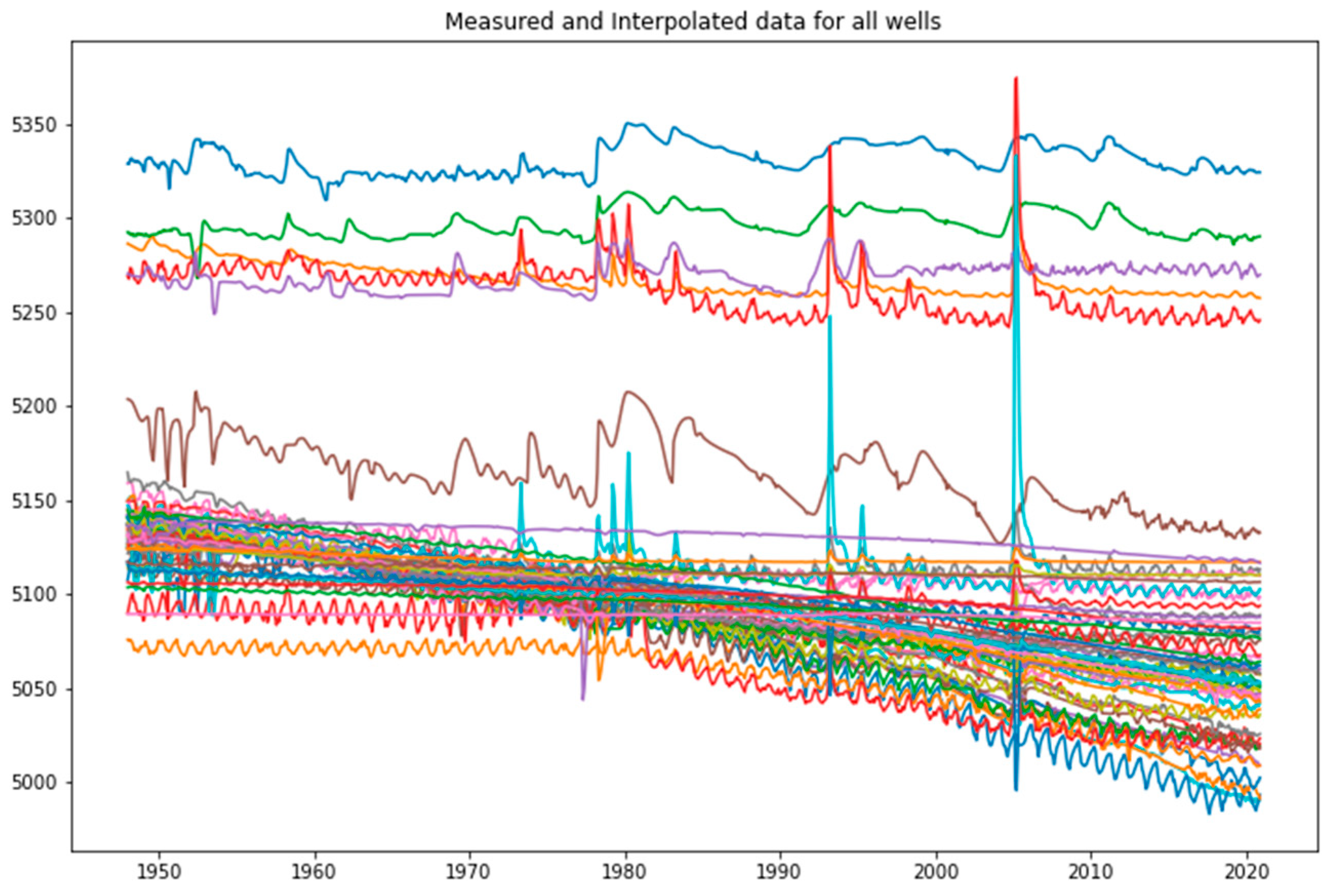
After imputation, at any location with an observed value, we replaced predictions with the observed value; this is known as direct insertion. Figure 14 shows the imputation results for all of the wells in the Beryl-Enterprise aquifer after direct insertion and imputed data for all missing values.

Figure 14 shows that several wells depict the same anomalies in 1993 and 2008, as shown in Figure 13. These wells have insufficient historical observations during this time, similar to the well presented in Figure 13. The general trend in the other wells shows that groundwater levels were generally increasing during this period, but these increases are not as extreme as these excursions.

Figure 14 seems to show that the five wells with significantly higher levels are in a different aquifer, though the data do not indicate this. These five wells show variation over imputation period, but no general trends. The wells exhibit a range of trends and structure; there appear to be two or three different pumping patterns in the aquifer in these complete datasets which were not as obvious in the observed data shown in Figure 10. This could be because the wells are used for different purposes, such as potable water supply or irrigation.

The use of induction bias to influence long-term trends and structure represents a significant step forward in this field. Imputation results generated without using these prior features do not typically express the long-term trends associated with groundwater data. The use of these priors for data with long gaps may not be accurate, as any long trend extrapolation can result in unrealistic values. However, this methodology provides a good initial estimate of the complete dataset for an aquifer representing groundwater storage changes. The method presented shows a way to develop priors based on the in situ data. Theoretically, different initial priors could be developed if the data-centric prior does not fit the specific bias of the researcher for the specific location. For these situations, the prior features would be extracted in the same way as presented once the initial prior is made, though justification would be required as to why a different initial prior better represents the situation.

These results show that the imputation method works well, even over long periods with no data. If the relationship between pumping, recharge, and climate changes, then the correlations modeled will not be stationary but change with time and, therefore, will not be representative of reality. As a result, seasonal trends or natural anomalies that do not appear in the original data may be lost or overrepresented in long periods with no data, causing large excursions, such as those shown in Figure 13. Nevertheless, the imputed values contain reasonable trends based on the observed data and hydrogeological principles. Even though there may be issues with individual wells during certain times, generally, the imputation depicts trends and structures shown by other wells with observed values in the aquifer.

5. Conclusions

Monitoring groundwater levels is important to determine the sustainable use of groundwater resources. It is difficult to obtain and manage groundwater data, and once a measurement has been missed, the record can no longer be obtained. To solve the problem of missing historical observations, we developed a groundwater imputation method that attempts to model groundwater levels by using a groundwater prior, namely meteorological variation from GLDAS, PDSI, and their embedded temporal components. We built a model that fits the groundwater observations based on the general shape of the prior, while containing the seasonal variation embedded in the meteorological data, using a multilayer perceptron. This was performed based on the assumption that groundwater moves slowly and observations in time are not necessarily independent from one another. This methodology showed great results over the Beryl-Enterprise aquifer in Utah where many wells were missing large periods of observations. Though this methodology was applied at Beryl-Enterprise, it can be used globally based on the global forcings, as long as quality groundwater observations exist.

We developed and presented our method for imputing missing groundwater data by using a case-study approach with 57 wells. We compared the resulting groundwater storage trends, estimated using wells with imputed data with another study of this aquifer. We did not directly compare our imputation method with other methods. To our knowledge, there are not any published descriptions of imputation methods specifically for well data, though there are many published data-imputation methods. A search on Google Scholar for “imputation” returns 687,000 results. Since well data are so varied, some are relatively stable, most have trends, some do not, some are periodic, and others are not, so it would be difficult to select candidate wells for a defensible comparison. We could easily select candidates to either show that our method was superior or show that another method was superior. Rather than comparing imputation methods, we felt that it was better to present our method by using a case study and then allow practitioners and researchers to decide if would be applicable to their data.

References

- Gleick, P.H. Water in Crisis: Paths to Sustainable Water Use. Ecol. Appl. 1998, 8, 571–579. [Google Scholar] [CrossRef]
- Kenny, J.F.; Barber, N.L.; Hutson, S.S.; Linsey, K.S.; Lovelace, J.K.; Maupin, M.A. Estimated Use of Water in the United States in 2005; US Geological Survey: Reston, VA, USA, 2009.
- Alsdorf, D.E.; Rodríguez, E.; Lettenmaier, D.P. Measuring Surface Water from Space. Rev. Geophys. 2007, 45, RG2002. [Google Scholar] [CrossRef]
- Butler, J.J.; Stotler, R.L.; Whittemore, D.O.; Reboulet, E.C. Interpretation of Water Level Changes in the High Plains Aquifer in Western Kansas. Groundwater 2013, 51, 180–190. [Google Scholar] [CrossRef]
- Beran, B.; Piasecki, M. Availability and Coverage of Hydrologic Data in the US Geological Survey National Water Information System (NWIS) and US Environmental Protection Agency Storage and Retrieval System (STORET). Earth Sci. Inform. 2008, 1, 119–129. [Google Scholar] [CrossRef]
- Glennon, R. The Perils of Groundwater Pumping. Issues Sci. Technol. 2002, 19, 73–79. [Google Scholar]
- Barbosa, S.A.; Pulla, S.T.; Williams, G.P.; Jones, N.L.; Mamane, B.; Sanchez, J.L. Evaluating Groundwater Storage Change and Recharge Using GRACE Data: A Case Study of Aquifers in Niger, West Africa. Remote Sens. 2022, 14, 1532. [Google Scholar] [CrossRef]
- Thomas, B.F.; Behrangi, A.; Famiglietti, J.S. Precipitation Intensity Effects on Groundwater Recharge in the Southwestern United States. Water 2016, 8, 90. [Google Scholar] [CrossRef]
- Bakker, M.; Schaars, F. Solving Groundwater Flow Problems with Time Series Analysis: You May Not Even Need Another Model. Groundwater 2019, 57, 826–833. [Google Scholar] [CrossRef]
- Rajaee, T.; Ebrahimi, H.; Nourani, V. A Review of the Artificial Intelligence Methods in Groundwater Level Modeling. J. Hydrol. 2019, 572, 336–351. [Google Scholar] [CrossRef]
- Coulibaly, P.; Anctil, F.; Aravena, R.; Bobée, B. Artificial Neural Network Modeling of Water Table Depth Fluctuations. Water Resour. Res. 2001, 37, 885–896. [Google Scholar] [CrossRef]
- Yoon, H.; Jun, S.-C.; Hyun, Y.; Bae, G.-O.; Lee, K.-K. A Comparative Study of Artificial Neural Networks and Support Vector Machines for Predicting Groundwater Levels in a Coastal Aquifer. J. Hydrol. 2011, 396, 128–138. [Google Scholar] [CrossRef]
- Emamgholizadeh, S.; Moslemi, K.; Karami, G. Prediction the Groundwater Level of Bastam Plain (Iran) by Artificial Neural Network (ANN) and Adaptive Neuro-Fuzzy Inference System (ANFIS). Water Resour. Manag. 2014, 28, 5433–5446. [Google Scholar] [CrossRef]
- Suryanarayana, C.; Sudheer, C.; Mahammood, V.; Panigrahi, B.K. An Integrated Wavelet-Support Vector Machine for Groundwater Level Prediction in Visakhapatnam, India. Neurocomputing 2014, 145, 324–335. [Google Scholar] [CrossRef]
- Karthikeyan, L.; Nagesh Kumar, D. Predictability of Nonstationary Time Series Using Wavelet and EMD Based ARMA Models. J. Hydrol. 2013, 502, 103–119. [Google Scholar] [CrossRef]
- Hussein, E.A.; Thron, C.; Ghaziasgar, M.; Bagula, A.; Vaccari, M. Groundwater Prediction Using Machine-Learning Tools. Algorithms 2020, 13, 300. [Google Scholar] [CrossRef]
- Asoka, A.; Gleeson, T.; Wada, Y.; Mishra, V. Relative Contribution of Monsoon Precipitation and Pumping to Changes in Groundwater Storage in India. Nat. Geosci. 2017, 10, 109–117. [Google Scholar] [CrossRef]
- Changnon, S.A.; Huff, F.A.; Hsu, C.-F. Relations between Precipitation and Shallow Groundwater in Illinois. J. Clim. 1988, 1, 1239–1250. [Google Scholar] [CrossRef]
- Petersen-Perlman, J.D.; Aguilar-Barajas, I.; Megdal, S.B. Drought and Groundwater Management: Interconnections, Challenges, and Policy Responses. Curr. Opin. Environ. Sci. Health 2022, 28, 100364. [Google Scholar] [CrossRef]
- Wang, F.; Lai, H.; Li, Y.; Feng, K.; Zhang, Z.; Tian, Q.; Zhu, X.; Yang, H. Identifying the Status of Groundwater Drought from a GRACE Mascon Model Perspective across China during 2003–2018. Agric. Water Manag. 2022, 260, 107251. [Google Scholar] [CrossRef]
- Evans, S.; Williams, G.P.; Jones, N.L.; Ames, D.P.; Nelson, E.J. Exploiting Earth Observation Data to Impute Groundwater Level Measurements with an Extreme Learning Machine. Remote Sens. 2020, 12, 2044. [Google Scholar] [CrossRef]
- Azizan, I.; Karim, S.A.B.A.; Raju, S.S.K. Fitting Rainfall Data by Using Cubic Spline Interpolation. MATEC Web Conf. 2018, 225, 05001. [Google Scholar] [CrossRef]
- Santopietro, S.; Gargano, R.; Granata, F.; de Marinis, G. Generation of Water Demand Time Series through Spline Curves. J. Water Resour. Plan. Manag. 2020, 146, 04020080. [Google Scholar] [CrossRef]
- Zaghiyan, M.R.; Eslamian, S.; Gohari, A.; Ebrahimi, M.S. Temporal Correction of Irregular Observed Intervals of Groundwater Level Series Using Interpolation Techniques. Theor. Appl. Climatol. 2021, 145, 1027–1037. [Google Scholar] [CrossRef]
- Dai, A. Dai Global Palmer Drought Severity Index (PDSI) 2017. Available online: https://climatedataguide.ucar.edu/climate-data/palmer-drought-severity-index-pdsi (accessed on 27 October 2022).
- Rodell, M.; Houser, P.R.; Jambor, U.; Gottschalck, J.; Mitchell, K.; Meng, C.-J.; Arsenault, K.; Cosgrove, B.; Radakovich, J.; Bosilovich, M.; et al. The Global Land Data Assimilation System. Bull. Am. Meteorol. Soc. 2004, 85, 381–394. [Google Scholar] [CrossRef]
- Palmer, W.C. Meteorological Drought; U.S. Department of Commerce, Weather Bureau: Silver Spring, MD, USA, 1965.
- Cook, E.R.; Seager, R.; Cane, M.A.; Stahle, D.W. North American Drought: Reconstructions, Causes, and Consequences. Earth-Sci. Rev. 2007, 81, 93–134. [Google Scholar] [CrossRef]
- Orwig, D.; Abrams, M. Variation in Radial Growth Responses to Drought Among Species, Site, and Canopy Strata. Trees-Struct. Funct. 1997, 11, 474–484. [Google Scholar] [CrossRef]
- Dai, A. Drought under Global Warming: A Review. WIREs Clim. Change 2011, 2, 45–65. [Google Scholar] [CrossRef]
- Dai, A.; Trenberth, K.E.; Qian, T. A Global Dataset of Palmer Drought Severity Index for 1870–2002: Relationship with Soil Moisture and Effects of Surface Warming. J. Hydrometeorol. 2004, 5, 1117–1130. [Google Scholar] [CrossRef]
- Vicente-Serrano, S.M.; López-Moreno, J.I. Hydrological Response to Different Time Scales of Climatological Drought: An Evaluation of the Standardized Precipitation Index in a Mountainous Mediterranean Basin. Hydrol. Earth Syst. Sci. 2005, 9, 523–533. [Google Scholar] [CrossRef]
- Khan, S.; Gabriel, H.F.; Rana, T. Standard Precipitation Index to Track Drought and Assess Impact of Rainfall on Watertables in Irrigation Areas. Irrig. Drain. Syst. 2008, 22, 159–177. [Google Scholar] [CrossRef]
- Dennison, P.E.; Brewer, S.C.; Arnold, J.D.; Moritz, M.A. Large Wildfire Trends in the Western United States, 1984–2011. Geophys. Res. Lett. 2014, 41, 2928–2933. [Google Scholar] [CrossRef]
- Lobell, D.B.; Roberts, M.J.; Schlenker, W.; Braun, N.; Little, B.B.; Rejesus, R.M.; Hammer, G.L. Greater Sensitivity to Drought Accompanies Maize Yield Increase in the U.S. Midwest. Science 2014, 344, 516–519. [Google Scholar] [CrossRef] [PubMed]
- Vicente-Serrano, S.M.; Beguería, S.; Lorenzo-Lacruz, J.; Camarero, J.J.; López-Moreno, J.I.; Azorin-Molina, C.; Revuelto, J.; Morán-Tejeda, E.; Sanchez-Lorenzo, A. Performance of Drought Indices for Ecological, Agricultural, and Hydrological Applications. Earth Interact. 2012, 16, 1–27. [Google Scholar] [CrossRef]
- Mishra, A.K.; Singh, V.P. A Review of Drought Concepts. J. Hydrol. 2010, 391, 202–216. [Google Scholar] [CrossRef]
- Karl, T.R. The Sensitivity of the Palmer Drought Severity Index and Palmer’s Z-Index to Their Calibration Coefficients Including Potential Evapotranspiration. J. Clim. Appl. Meteorol. 1986, 25, 77–86. [Google Scholar] [CrossRef]
- Ramirez, S.G.; Hales, R.C.; Williams, G.P.; Jones, N.L. Extending SC-PDSI-PM with Neural Network Regression Using GLDAS Data and Permutation Feature Importance. Environ. Model. Softw. 2022, 157, 105475. [Google Scholar] [CrossRef]
- Rui, H.; Beaudoing, H.; Loeser, C. README for NASA GLDAS Version 2 Data Products; NASA Goddard Space Flight Center: Greenbelt, MD, USA, 2021; p. 22.
- Landerer, F.W.; Flechtner, F.M.; Save, H.; Webb, F.H.; Bandikova, T.; Bertiger, W.I.; Bettadpur, S.V.; Byun, S.H.; Dahle, C.; Dobslaw, H.; et al. Extending the Global Mass Change Data Record: GRACE Follow-On Instrument and Science Data Performance. Geophys. Res. Lett. 2020, 47, e2020GL088306. [Google Scholar] [CrossRef]
- Rzepecka, Z.; Birylo, M. Groundwater Storage Changes Derived from GRACE and GLDAS on Smaller River Basins—A Case Study in Poland. Geosciences 2020, 10, 124. [Google Scholar] [CrossRef]
- McStraw, T.C.; Pulla, S.T.; Jones, N.L.; Williams, G.P.; David, C.H.; Nelson, J.E.; Ames, D.P. An Open-Source Web Application for Regional Analysis of GRACE Groundwater Data and Engaging Stakeholders in Groundwater Management. JAWRA J. Am. Water Resour. Assoc. 2021. [Google Scholar] [CrossRef]
- Dunbar, B. “GRACE Mission”. Spacecraft. Available online: http://www.nasa.gov/mission_pages/Grace/spacecraft/index.html (accessed on 4 January 2022).
- Wahr, J.; Molenaar, M.; Bryan, F. Time Variability of the Earth’s Gravity Field: Hydrological and Oceanic Effects and Their Possible Detection Using GRACE. J. Geophys. Res. Solid Earth 1998, 103, 30205–30229. [Google Scholar] [CrossRef]
- Géron, A. Hands-On Machine Learning with Scikit-Learn, Keras, and TensorFlow, 2nd ed.; O’Reilly Media, Incorporated: Sebastopol, CA, USA, 2019. [Google Scholar]
- EmilienDupont Interactive Visualization of Optimization Algorithms in Deep Learning. Available online: https://emiliendupont.github.io/2018/01/24/optimization-visualization/ (accessed on 1 February 2021).
- Abadi, M.; Barham, P.; Chen, J.; Chen, Z.; Davis, A.; Dean, J.; Devin, M.; Ghemawat, S.; Irving, G.; Isard, M.; et al. TensorFlow: A System for Large-Scale Machine Learning. In Proceedings of the 12th USENIX Symposium on Operating Systems Design and Implementation (OSDI’16), Savannah, GA, USA, 2–4 November 2016; p. 21. [Google Scholar]
- Chollet, F. Deep Learning with Python; Manning Publications, Co.: Shelter Island, NY, USA, 2018; ISBN 978-1-61729-443-3. [Google Scholar]
- Mower, R.W.; Sandberg, G.W. Hydrology of the Beryl-Enterprise Area, Escalante Desert, Utah, with Emphasis on Ground Water; With a Section on Surface Water; Technical Publication; Utah Department of Natural Resources, Division of Water Rights: Salt Lake City, UT, USA, 1982; Volume 73, p. 86.
- Farr, T.G.; Rosen, P.A.; Caro, E.; Crippen, R.; Duren, R.; Hensley, S.; Kobrick, M.; Paller, M.; Rodriguez, E.; Roth, L.; et al. The Shuttle Radar Topography Mission. Rev. Geophys. 2007, 45, RG2004. [Google Scholar] [CrossRef]
- USGS Water Data for the Nation. Available online: https://waterdata.usgs.gov/nwis (accessed on 22 May 2022).
- Freeze, R.A.; Cherry, J.A. Groundwater; Prentice-Hall: Hoboken, NJ, USA, 1979; ISBN 978-0-13-365312-0. [Google Scholar]
Publisher’s Note: MDPI stays neutral with regard to jurisdictional claims in published maps and institutional affiliations. |
© 2022 by the authors. Licensee MDPI, Basel, Switzerland. This article is an open access article distributed under the terms and conditions of the Creative Commons Attribution (CC BY) license (https://creativecommons.org/licenses/by/4.0/).