Article

Assimilation of Deep Learning and Machine Learning Schemes into a Remote Sensing-Incorporated Crop Model to Simulate Barley and Wheat Productivities

1
Department of Applied Plant Science, Chonnam National University, Gwangju 61186, Korea
2
Satellite Application Division, Korea Aerospace Research Institute, Daejeon 34133, Korea
3
Department of Agricultural Environment, National Institute of Agricultural Science, Wanju-gun 55365, Korea
4
Department of Agricultural Science, Gyeongsang National University, Jinju 52828, Korea
*
Author to whom correspondence should be addressed.
These authors contributed equally to this work.
Remote Sens. 2022, 14(21), 5443; https://doi.org/10.3390/rs14215443
Submission received: 29 August 2022 / Revised: 19 October 2022 / Accepted: 26 October 2022 / Published: 29 October 2022

Abstract

:
Deep learning (DL) and machine learning (ML) procedures are prevailing data-driven schemes capable of advancing crop-modelling practices that assimilate these techniques into a mathematical crop model. A DL or ML modelling scheme can effectively represent complicated algorithms. This study reports on an advanced fusion methodology for evaluating the leaf area index (LAI) of barley and wheat that employs remotely sensed information based on deep neural network (DNN) and ML regression approaches. We investigated the most appropriate ML regressors for exploring LAI estimations of barley and wheat through the relationships between the LAI values and four vegetation indices. After analysing ten ML regression models, we concluded that the gradient boost (GB) regressor most effectively estimated the LAI for both barley and wheat. Furthermore, the GB regressor outperformed the DNN regressor, with model efficiencies of 0.89 for barley and 0.45 for wheat. Additionally, we verified that it would be possible to simulate LAI using proximal and remote sensing data based on assimilating the DNN and ML regressors into a process-based mathematical crop model. In summary, we have demonstrated that if DNN and ML schemes are integrated into a crop model, they can facilitate crop growth and boost productivity monitoring.

1. Introduction

Deep neural networks (DNNs) and machine learning (ML) can be assimilated into a mathematical crop modelling system integrated with remote sensing (RS) information. The DNN and ML techniques have been recognised as practical schemes for resolving the many problems of conventional empirical modelling approaches to crop yield simulations that use RS data because they consider the nonlinearity between input variables and yields [1,2,3]. Previous investigations have attempted to integrate an ML structure with crop models to develop an estimation of yield [4,5,6]. These investigations consisted of crop model variables that were used as input features in ML models. It has also been reported that recent improvements in DNN methodologies based on their influential estimate performance can be applied to increasingly advanced and precise crop yield simulations [7,8,9]. The DNN and ML methodologies employed to crop yield prediction include the support vector machine, random forests (RFs), convolutional neural networks, and long short-term memory. Additionally, DNN and ML schemes can facilitate mathematical crop-modelling methodologies to assimilate them into a mathematical crop model so as to replicate and predict the morphogenesis of crops [10].
RS has also proven to be a valuable technique for monitoring crop growth and development conditions influenced by geographic and spatial inconsistencies during crop-growing seasons [11]. RS techniques help acquire crop growth data for specific geographical areas of interest. Despite temporal limitations in observational scouting, and depending on the platform, RS can be useful for analysing active spatial variations in crop morphogenesis within agricultural ecosystems [12]. Crop morphogenesis conditions and yields can be evaluated by investigating the associations between crop growth variables and RS information [12,13,14]. For example, many studies have been conducted on estimating crop yields using optical RS data based on empirical modelling [15,16]. Such modelling structures are both practical and suitable for determining growth conditions and productivity in specific regions. However, these empirical modelling procedures cannot adequately describe the morphogenesis (i.e., the growth and development courses) of plants or their influences on productivity [17,18].
Process-based crop models are articulated using mathematical formulations to simulate progression in crop growth and development conditions [19,20]. While these crop models can present consistent modelling performance, gathering numerous spatial inputs and complex crop-specific coefficients for geospatial simulation can significantly limit the effectiveness of the models [21].
A fusion approach that assimilates RS information into a crop model could strengthen both methodologies and compensate for each specific strategy’s limitations, minimising the discrete performances or spatiotemporal gaps for both RS-observed and model-simulated information [22,23]. Widespread investigative efforts have advanced crop-modelling practices by integrating RS information into a crop model using multiple data integration techniques linking crop-modelling and RS [23,24,25]. For example, the RS-incorporated crop model (RSCM) was formulated as a result of a synthesis scheme that can simulate agronomic crops such as barley, paddy rice, soybeans, and wheat [23,26,27,28]. Furthermore, the RSCM system can integrate the leaf area index (LAI) or RS-based vegetation indices (VIs) from different operational platforms.
The LAI is an essential variable for crop simulation in most process-based mathematical crop models. It can be combined with RS data using mathematical optimisation procedures [23,24,25]. For example, the LAI variable in the RSCM scheme was developed using a linear mathematical relationship with VIs achieved from different RS platforms [23,26,29,30,31]. Nevertheless, formulating stable mathematical equations can present challenges, which mainly comprise differences in a plant canopy dimension (D) between LAI (i.e., 3D) and VIs (i.e., 2D) or likely discrepancies in the associations between various RS platforms and associated dynamic inconsistencies among crop cultivars. These differences even appear in various growth stages, especially when leaf senescence occurs. An innovative approach is, therefore, necessary to estimate consistent LAI values and to improve the functioning of mathematical crop models incorporated with RS information and the RSCM.
Both DNN and ML approaches are expected to assist in the advancement of the simulation performances of current process-based crop models via the efficient integration of data-driven modelling procedures. Although earlier fusion efforts were able to include crop simulation variables in DNN and ML models [10], further studies will be necessary to more effectively amalgamate these processes into a mathematical crop model. Therefore, the overall goal of the current study was to develop an advanced fusion methodology that can integrate DNN and ML procedures into a mathematical crop model based on estimations of the LAI values of barley and wheat. We researched appropriate DNN and ML models to calculate the LAI values of barley and wheat per the relationship between LAI and RS-based VIs. We employed an ensemble approach in the relationship investigation using four structural VIs rather than a single VI to integrate the advantage of the unique features of each VI.

2. Materials and Methods

2.1. Field Experiment

The field experiment took place at Gyeongsang National University (GNU; 35°8′N, 128°5′E; 33 m) in Jinju, South Gyeongsang Province, Republic of Korea, during the barley and wheat seasons from 2018 to 2021. Its aim was to assess the model coefficients and achieve datasets for assessing the modelling system. The study site experiences a characteristic East Asian monsoon weather condition. Average yearly temperatures and mean annual precipitation rates have been recorded as 13.1 °C and 1513 mm, respectively, during the previous 30 years by the Korea Meteorological Administration (https://www.kma.go.kr/eng/, accessed on 20 August 2022). Approximately 60% of the annual rainfall occurs in the summer monsoonal periods from July to August. The topsoil zone (0–20 cm) is categorised as a sandy loam (9.7% clay, 18.8% silt, and 71.4% sand), with an organic carbon content of 8.6 g C kg1, a pH of 5.9, available phosphorus (P) of 185 mg P2O5 kg1, a cation exchange capacity of 6.3 cmolc kg1, and entire nitrogen content before fertilisation of 0.053 g N kg−1, as stated by the National Institute of Agricultural Sciences (www.naas.go.kr/english/, accessed on 20 August 2022).
A wheat cultivar, Chokyung, and a barley cultivar, Heenchal, were sown between 30 October and 5 November for autumn seeding (18–20 February for spring seeding) and harvested between 7 and 25 June (Table 1) over an area of approximately 714 m2. Additional information regarding the respective crop varieties can be accessed through the National Institute of Crop Science (www.nics.go.kr/english/, accessed on 20 August 2022). The N fertiliser for the standard treatment in this study was set at an amount of 100 kg ha−1 for wheat and 80 kg ha−1 for barley, with 40% dispersed beneath the soil surface as a basal quantity before sowing and 30% used at the tillering and panicle initiation phases as a side dressing. In addition, potassium (K) and P fertilisers were treated at 70 and 35 kg ha−1 for both barley and wheat, respectively. Before seeding, the K and P fertilisers were dispersed beneath the soil surface as a basal treatment. The N treatments during each crop season involved three varying applications. The N treatments for wheat were 40% (40 kg ha−1) at seeding, 30% (30 kg ha−1) at rejuvenation, and 0% (0 kg ha−1) at early reproduction (N40-30-0), N40-30-30, and N40-30-60. The treatments for barley were 40% (34 kg ha−1) at seeding, 30% (24 kg ha−1) at rejuvenation, and 30% (24 kg ha−1) at early reproduction (N40-30-30). All the experimental blocks were arranged in a completely randomised block design in three duplications for each crop field. The barley and wheat were seeded in a 0.2 m row spacing and a 0.1 m hill-to-hill spacing using a mechanical seed drilling hand machine.
The LAI was determined using an LAI-2200C (LI-COR Inc., Lincoln, NE, USA) during the primary barley and wheat development stages. The LAI-2200C can measure the LAI of a canopy below diffuse or direct sunlight via its light-diffusing cover and light-scattering rectification scheme, providing accurate and comprehensive results. LAI was calculated five or six times during the crop-growing season (Table 1) and three times for each plot.
Weather conditions at the research site were automatically recorded using a mechanical MetPRO (Campbell, Logan, UT, USA) weather station. The diurnal solar radiation, average mean temperature, and precipitation ranged from 11.81–15.81 MJ m−2 d−1, 8.28–15.96 °C, and 1.95–2.96 mm d−1, respectively, throughout the crop-growing period (Table 1).

2.2. Proximal and UAS-Based Remote Sensing Data

We collected proximal sensing information on the ground and from the unmanned aerial system (UAS) RS images at the study site between 2018 and 2021. All field operations to determine the barley and wheat canopy reflectances were carried out either an hour before or after the local solar noon (12:40 pm KST) to minimise the potential perspective influences on the plants of an image of interest or sensing scene. We measured canopy reflectance to define the barley and wheat growth conditions during the primary development stages using an MSR16R (CROPSCAN, Inc., Rochester, MN, USA), a portable multispectral radiometer. The MSR16R can quantity the reflectance values at 16 wavebands ranging from 450 to 1750 nm. The proximal sensing practices were carried out on dates matching the LAI measurements (Table 1) to obtain vegetation indices (VIs) through the use of canopy reflectances at wavebands of 560, 660, and 800 nm. The VIs of interest were the normalised difference vegetation index (NDVI) [32], the optimised soil-adjusted vegetation index (OSAVI) [33], the modified triangular vegetation index 1 (MTVI1) [34], and the re-normalised difference vegetation index (RDVI) [35]. The VIs were determined using the following calculations:
MTVI1 = 1.2·[1.2·(ρ800ρ660) − 2.5·(ρ660ρ560)]
NDVI = (ρ800ρ660)/(ρ800 + ρ660)
OSAVI = (ρ800ρ660)/(ρ800 + ρ560 + 0.16)
RDVI = ( ρ 800 ρ 660 ) / ( ρ 800 + ρ 660 )
where ρ560, ρ660, and ρ800 represent reflectances at 560, 660, and 800 nm, respectively.
A UAS, eBee (senseFly, Cheseaux-sur-Lausanne, Switzerland), was employed to acquire remotely controlled airborne sensing images for the barley and wheat fields. The UAS weighted 700 g, had a wing length of 960 mm, and was equipped with a Powershot S110 NIR digital camera (Canon, Inc., Tokyo, Japan) with a 12.1 MP sensor and three spectral bands (green at the centre band (CB) of 550 nm, red at the CB of 625 nm, and near-infrared at the CB of 850 nm). UAS RS images were obtained six times throughout the crop-growing season each year (Table 1). First, these UAS RS data were radiometrically corrected and mosaicked using a Pix4D mapper (Pix4D S.A., Prilly, Switzerland) to characterise barley and wheat growth conditions for all experimental field scenes. Next, the radiometrically rectified UAS images were geometrically adjusted using ERDAS IMAGINE (Hexagon Geospatial, Madison, AL, USA). Finally, the image data were georeferenced and registered using ArcGIS (ESRI, Inc., Redlands, CA, USA).

2.3. Model Design

The RSCM for barley and wheat employed in this study is a simple crop model integrated with either an ML or DNN regressor based on specific crop growth parameters using a mathematical optimisation procedure (Figure 1). We combined the DNN and ML regressors into the RSCM system in line with the investigations of the DNN or ML regressors outlined in the subsequent subsection. The DNN and ML procedures improved the mathematical regression method for the LAI and RS-based VIs relationships.
The RSCM scheme implements several mathematical calculations incorporating growth-specific coefficients to simulate growth and grain yield using a radiation use efficiency (RUE) approach [36]. The growth-specific coefficients comprise base temperature, leaf partitioning and senescence function parameters, radiation extinction coefficient (k), RUE, and specific leaf area (Figure A1). The modelling schemes used the same barley and wheat growth-specific parameters determined in earlier studies [27,28].
The RSCM can adapt the crop growth-specific model parameters to replicate the growth variables according to the within-season calibration procedure, which can compare the simulation with the observation of readily available crop state variables (i.e., LAI) and adjust the model parameters [23]. This procedure uses POWELL optimisation [37] or quasi-Newton minimisation calculations [38] to achieve a mathematical agreement between the simulated and observed LAI. This mathematical procedure optimises the simulated and observed LAIs using the crop growth-specific parameters (L0, a, b, and c) describing canopy growth processes. Furthermore, the mathematical procedure calibrates all parameters to ensure congruence between simulations and observations. The updated RSCM system also employed this within-season calibration procedure to input RS-observed or ML and DNN-estimated LAI data (Figure 1). The within-season calibration procedure was formulated to moderate the uncertainties in crop modelling induced by probable inaccuracies or the unapproachability of state variables such as LAI [39]. In addition, the crop growth-specific coefficients can be rectified using the Bayesian process to gain suitable values with a prior distribution in accordance with the estimates provided by previous studies [23,40].

2.4. DNN and ML Regression Models

We investigated 10 ML models and DNN model regressors. The ML models comprised Extra Trees (ET), Extreme Gradient Boosting (XGB), Gradient Boosting (GB), Histogram-based Gradient Boosting (HGB), Least Absolute Shrinkage and Selection Operator (LASSO), Light Gradient Boosting Machine (LGBM), Polynomial Regression, RF, Ridge, and Support Vector Regression (SVR) regressors. All the ML and DNN models adopted have the features of a statistic regressor [10]. The models are accessible as Python packages (https://www.python.org/, accessed 20 August 2022). In addition, the ML models are contained within the Scikit-learn module (https://scikit-learn.org/, accessed on 20 August 2022), while the DNN model is included in the Keras model (https://keras.io/, accessed on 20 August 2022).
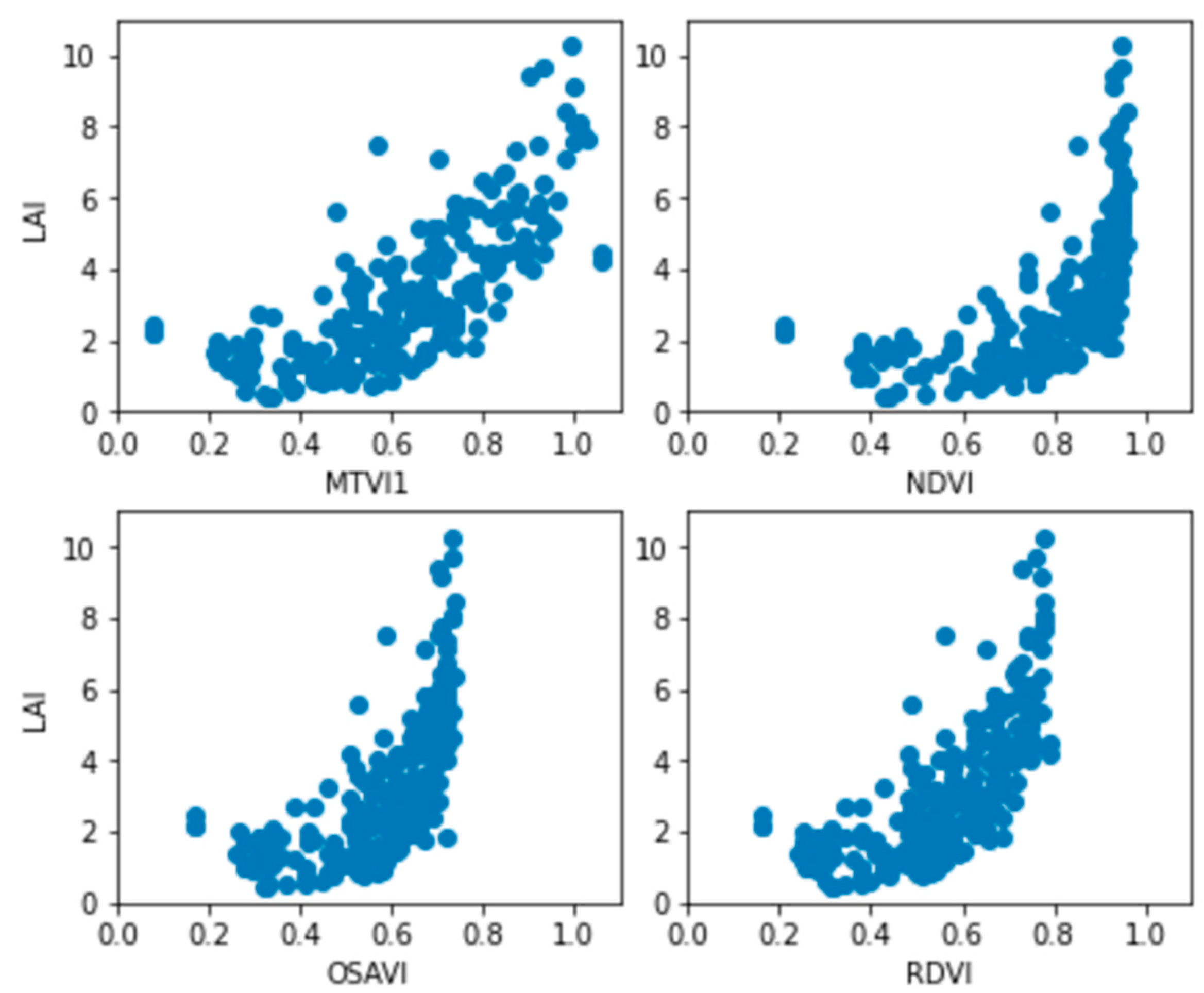
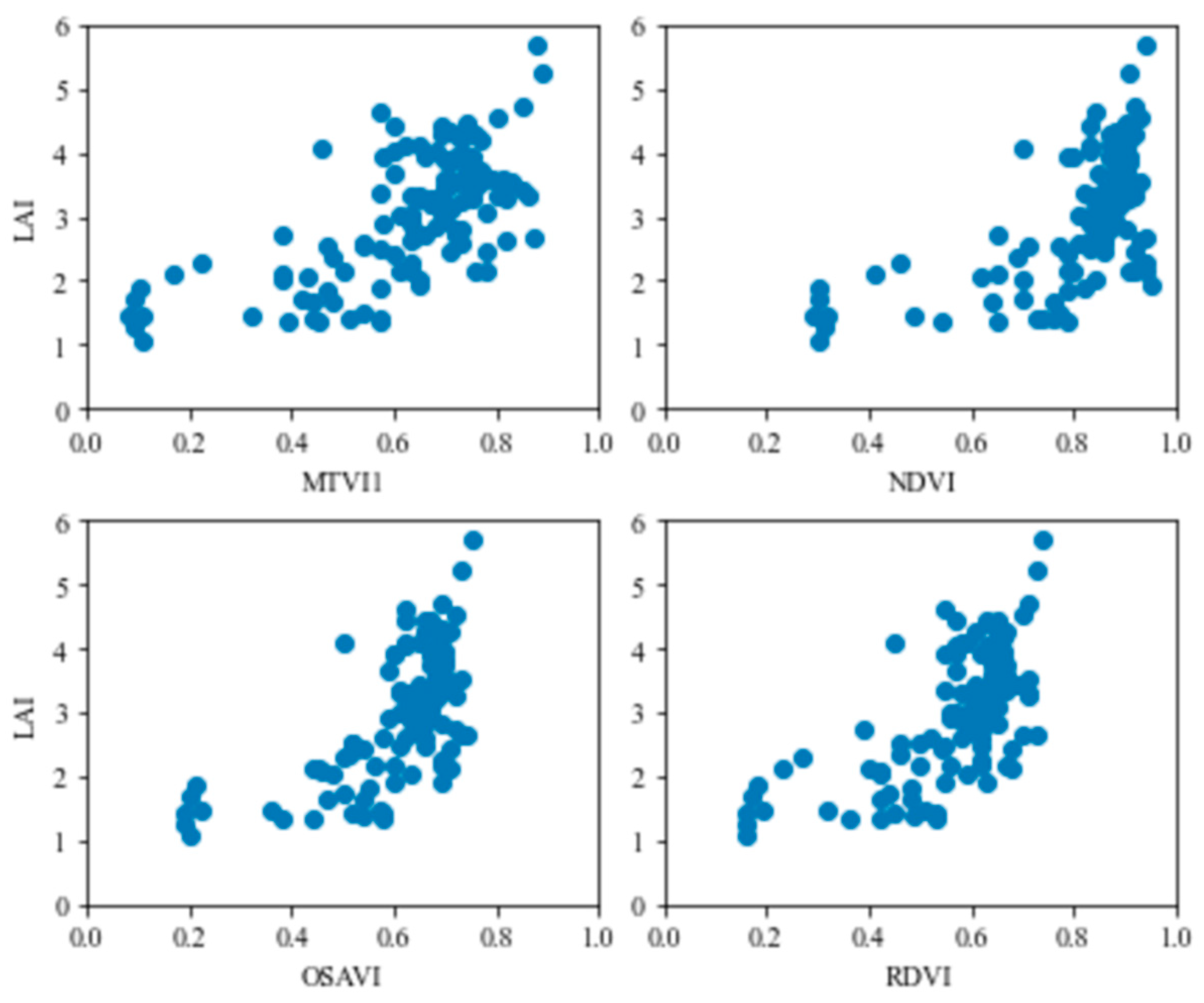
The current study used proximal and UAS-based RS VIs to estimate LAI values during the barley and wheat growing seasons by utilising the DNN and ML regressors. Three annual datasets from 2018 to 2020 were utilised to build the DNN and ML models, and the 2021 dataset was employed for model evaluation. We simulated the LAI values using the DNN and ML-based empirical relationships between LAI and the proximally sensed VIs for both barley (Figure 2) and wheat (Figure 3). The datasets employed for model development were separated into training and test sets with ratios of 0.7 and 0.3, respectively, using the Scikit-learn ML design. The regression models were trained and tested in order to define suitable hyperparameters. Alpha values for LASSO and Ridge were estimated as 0.0001 by both regressors for barley and 0.001 and 10 for wheat according to a grid search approach with a specific value range (Figure A2). The activation function used by the DNN models for both barley and wheat was the rectified linear unit (ReLU), which applied six fully connected layers with a design of gradually incrementing and reducing units from 100 to 1000 (Figure A3). The models were performed with dropout rates of 0.17 for barley and 0.19 for wheat while adopting the ‘RMSprop’ optimiser at a learning rate of 0.001 with 500 epochs and a batch size of 100. We employed grid search and trial-and-error approaches to defining the DNN hyperparameters, seeking minimum and steady root mean square errors for barley and wheat (Figure A4).

2.5. Model Evaluation

We adopted four statistical indices to assess the RSCM system’s performance: a p-value determined by a two-sample t-test, mean absolute error (MAE), root mean squared deviation (RMSD), and Nash–Sutcliffe model efficiency (ME) [41]. We used the Python statistics module to calculate MAE, RMSD, and ME based on the following formulas:
M A E = i = 1 n | S i O i | n
R M S D = 1 n i = 1 n ( S i O i ) 2
M E = 1 i = 1 n ( S i O i ) 2 i = 1 n ( O i O m ) 2
where Si, Oi, Om, and n show the simulated value, the observed value, the mean observed value, and the whole number of observations, respectively. ME values can range from −∞ to 1. An ME value closer to 1 specifies greater reliability of the model. An ME value less than 0 indicates more consistency in the observation but poor reliability of the model. We also adopted normalised ME (NME) for more advanced analysis, permitting the ME measurement in model validation methods. Thus, ME = 1, 0, and −∞ matches with NME = 1, 0.5, and 0, respectively.

3. Results

3.1. DNN and ML Evaluation

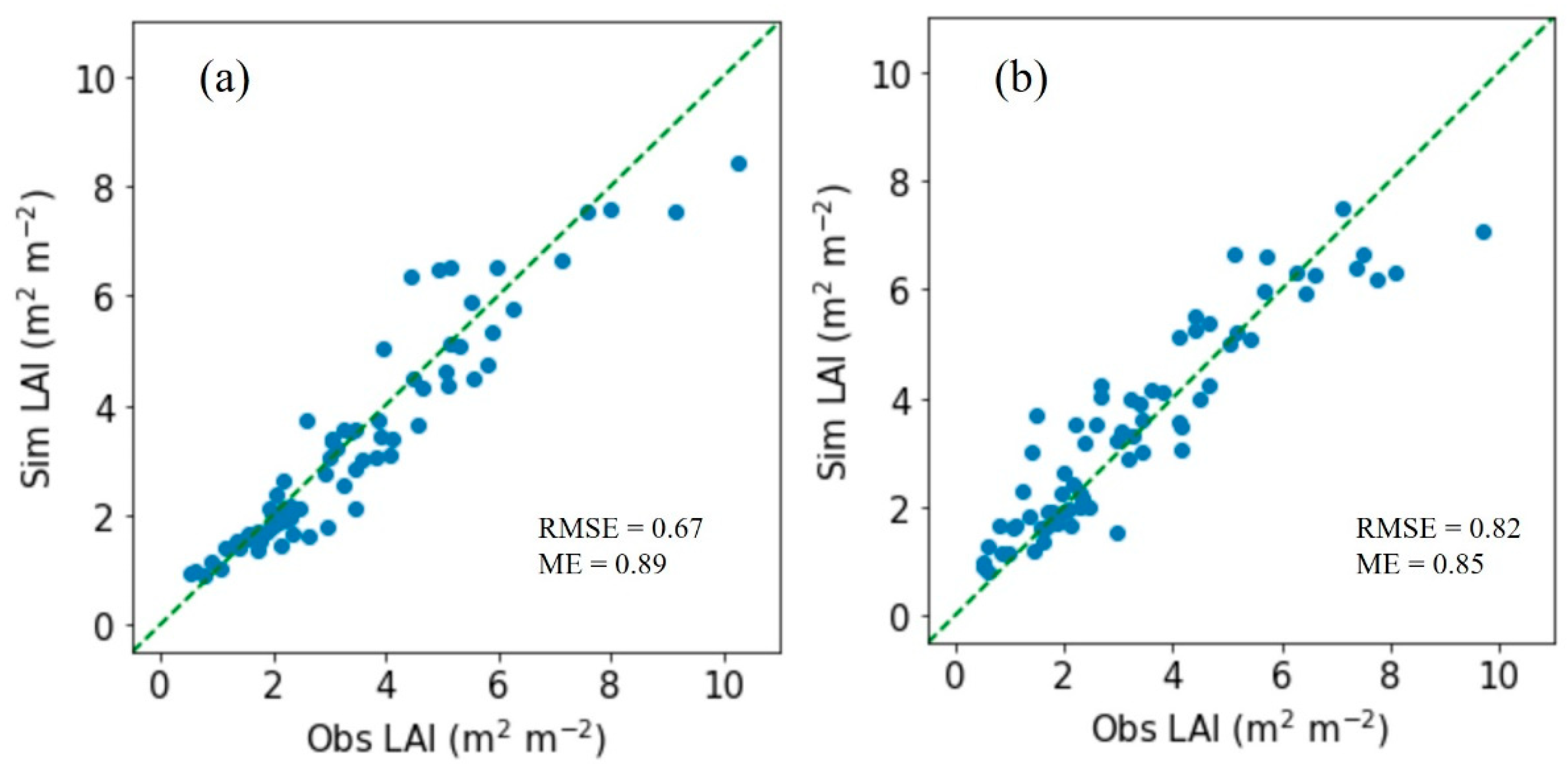
The training scores using 10 ML regression models for LAI regression analyses in relation to VIs for barley were 0.872–0.999, whereas the test scores ranged from 0.759 to 0.814 (Table 2). On the other hand, the training scores for wheat ranged between 0.542 and 0.999, while the test scores ranged between 0.335 and 0.685. Therefore, the GB regressor was considered as the optimal model for both crops according to training and test performances and its capacity for simulating the LAI in comparison with the DNN model was analysed. Simulated LAI values for wheat concurred with the matching observed LAI values, with an RMSD of 0.71 m2 m2 and an ME of 0.45 using the GB regression and an RMSD of 0.64 m2 m2 and an ME of 0.41 using the DNN regression (Figure 4 and Table 2). Additionally, the simulated LAI values for barley aligned with the observed LAI values, with an RMSD of 0.67 m2 m2 and an ME of 0.89 for the GB regression and an RMSD and ME of 0.82 m2 m2 and 0.85, respectively, for the DNN structure (Figure 5 and Table 3).

3.2. RSCM Evaluation

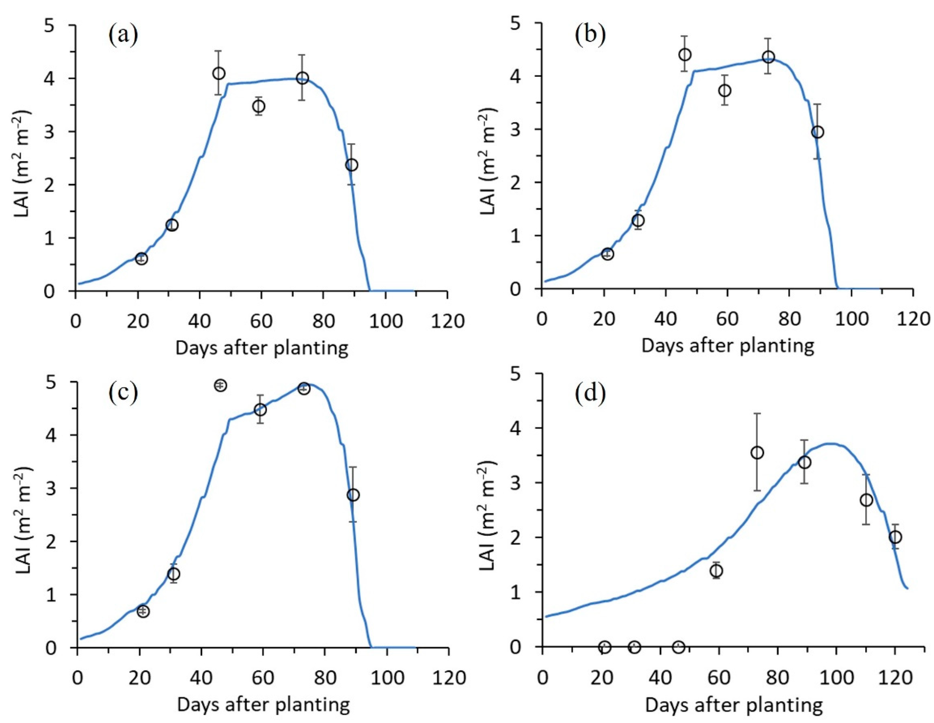
The GB and DNN-projected LAI values were used to simulate the LAI and grain yields of wheat (Figure 6) and barley (Figure 7) employing the RSCM regime. Consequently, the estimated LAI values matched the observed LAI values with MAEs of 0.29, 0.31, and 0.35 m2 m−2; RMSDs of 0.39, 0.41, and 0.52 m2 m−2; and MEs of 0.919, 0.925, and 0.906 for the different N treatments for the autumn-seeded wheat (Table A1). In addition, the simulated and observed LAI values matched, with an MAE of 0.44 m2 m−2, an RMSD of 0.54 m2 m−2, and an ME of 0.631 for the spring-seeded wheat. Likewise, simulated grain yields aligned significantly with the observed grain yields (p = 0.850, 0.537, and 0.669) as shown by the t-tests with MAEs of 0.659, 0.546, and 0.840 tonne ha−1; RMSDs of 0.754, 0.594, and 1.129 tonnes ha−1; and NMEs of 1.000, 0.995, and 0.998 for the different N treatments for the autumn-seeded wheat (Table 4). Simulated and observed grain yields also showed significant agreement (p = 0.922) as shown by the t-test, with an MAE of 0.543 tonne ha−1, an RMSD of 0.592 tonne ha−1, and an NME of 0.790 for the spring-sown wheat.
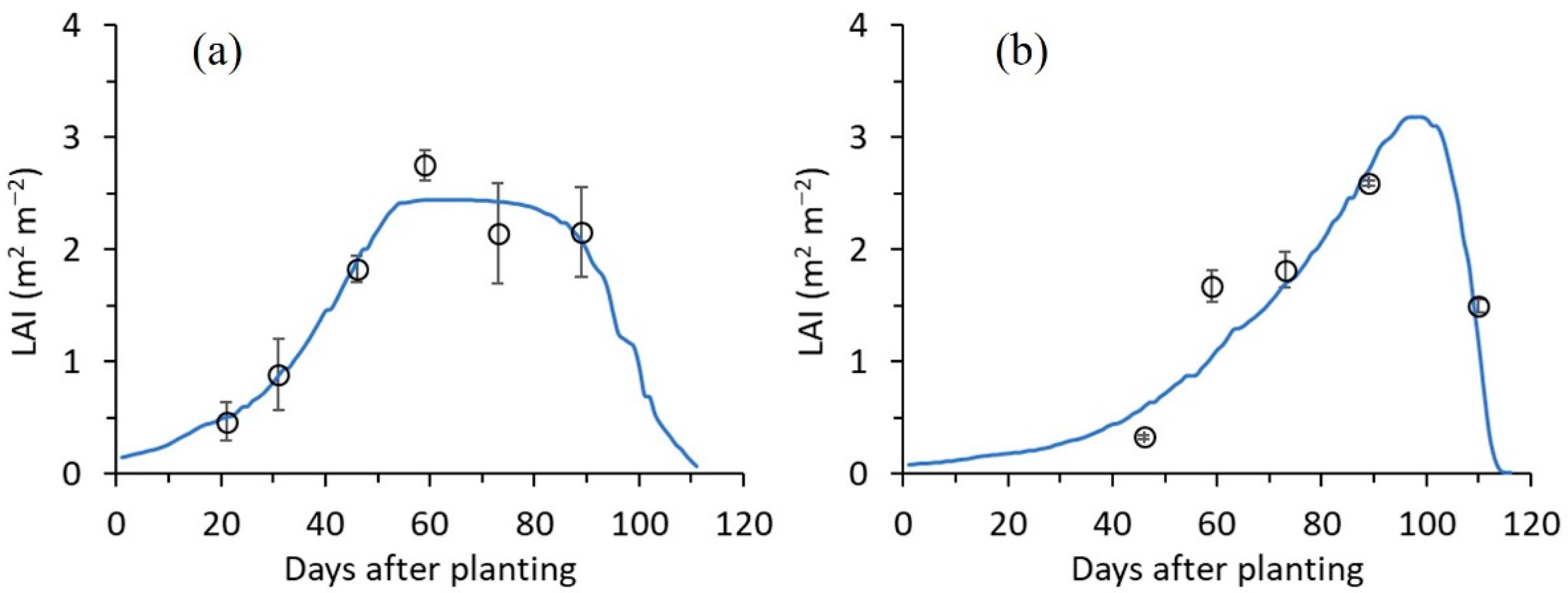
The simulated LAI values matched the observed LAI values, with MAEs of 0.16 and 0.32 m2 m−2, RMSDs of 0.21 and 0.37 m2 m−2, and MEs of 0.938 and 0.766 for the autumn and spring-sown barley, respectively (Figure 7 and Table A1). Likewise, simulated grain yields agreed significantly with the measured grain yields (p = 0.825 and 0.007) according to two-sample t-tests, with MAEs of 0.519 and 0.211 tonne ha−1, RMSDs of 0.559- and 0.212 tonne ha−1, and NMEs of 0.989 and 0.0 for the autumn and spring-sown barley, respectively (Table 5).

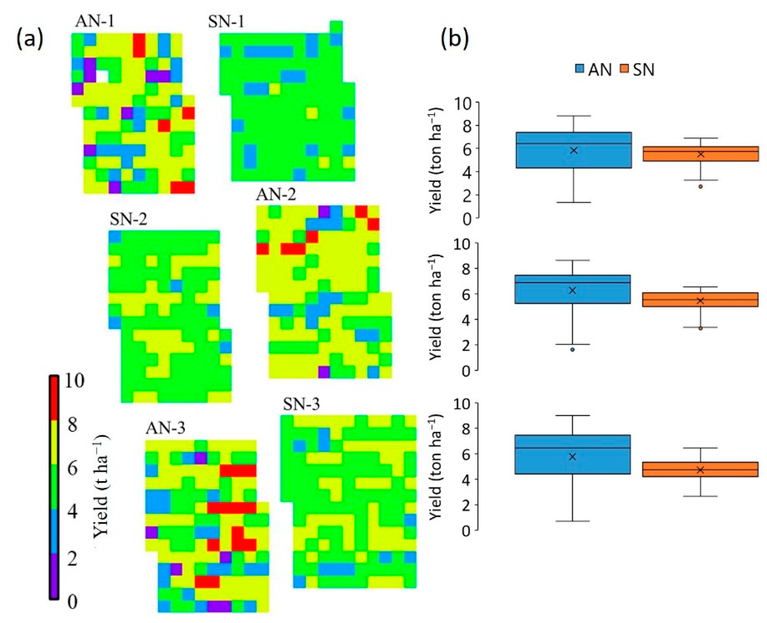
3.3. Geographical Projection

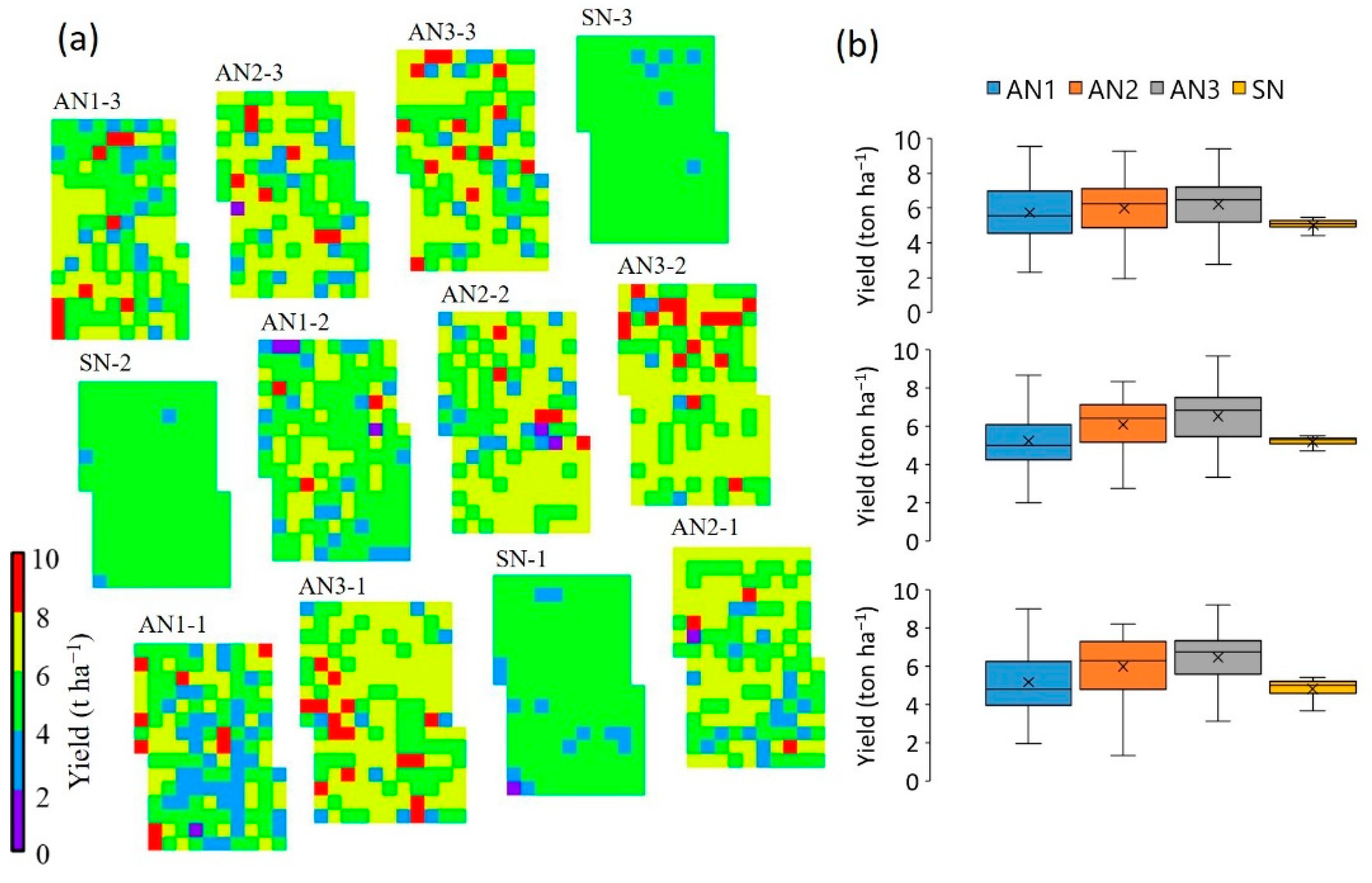
We found that the RSCM system could simulate spatiotemporal field variations in the grain yields of wheat and barley (Figure 8 and Figure 9). Wheat yields were reproduced with mean ± one standard deviation values of 5.381 ± 1.505 tonne ha−1 for AN1 (autumn seeding, N30-30-0 kg ha−1), 6.021 ± 1.441 tonne ha−1 for AN2 (autumn seeding, N30-30-30 kg ha−1), 6.401 ± 1.379 tonne ha−1 for AN3 (autumn seeding, N30-30-60 kg ha−1), and 5.008 ± 0.438 tonne ha−1 for SN (spring seeding, N30-30-30 kg ha−1) treatments (Figure 8).
Barley yields were reproduced with mean ± one standard deviation values of 5.962 ± 1.893 tonne ha−1 for AN (autumn seeding, N24-24-32 kg ha−1) and 5.236 ± 0.789 tonne ha−1 for SN (spring seeding, N24-24-32 kg ha−1) treatments (Figure 9).

4. Discussion

The current study investigated how effectively DNN and ML approaches could be assimilated into a process-based mathematical crop model. To perform this investigation, we developed a mixed crop-modelling methodology using effective DNN and ML techniques to replicate barley and wheat LAI values using plant structural VIs based on datasets to advance crop-modelling practices. We found that the ET model was the optimal ML regressor for simulating the barley and wheat LAI values and that it was superior to the DNN regressors. While this study’s findings closely resemble those of a recent report [10], they generally conflict with earlier research that showed the DNN approaches outperforming the best ML approaches [42,43]. Therefore, the simulation consequences may depend on the data scope and accompanying characteristics attributed to study cases. However, if a broader range of data is applied in future studies than was used in our approach, the DNN regressor may prove to be as effective as it was in previous studies [42,43].
Our study also evaluated and tested the RSCM system, which integrated proximal and RS information to simulate the spatiotemporal variations in barley and wheat growth and grain yield. The simulation outcome using the updated RSCM regime verified that it could reproduce temporal variations in barley and wheat growth and grain yield in fields. Furthermore, by using UAS-based RS imagery, the simulation results showed that the RSCM could simulate spatiotemporal variations in grain yield induced by field conditions. Our findings also confirmed the ability of the RSCM to use LAI data to minimise inaccuracies between simulated and observed canopy growth variables.
Crop models are typically designed to simulate crop responses to environmental conditions, thus helping examine ideal crop growth and best management practices [44]. Some endeavours made by crop modellers were meant to develop parameter estimation protocols in order to simplify crop models and minimise differences between simulations and measurements [22,45]. A sufficiently adjusted crop model should precisely replicate crop growth and development, output, and associated environmental factors [45].
The RSCM system is designed to perform the parameter optimisation function and replicate crop growth and productivity using modest input requirements by assimilating proximal sensing or RS information [23]. Researchers have attempted to establish similar integrated crop-modelling regimes for different staple crops, including barley [27], cotton [46], rice [30], soybeans [26], and wheat [28]. The proposed RSCM system could accurately simulate barley and wheat productivities under different planting and N application regimes to a statistically significant degree. We showed that RSCM-simulated LAI and grain yield values correlated significantly with the equivalent measured values. The RSCM system can be used to determine suitable seeding and N applications and simulate geospatial variations in yield based on pixel-based two-dimensional simulations. Therefore, integrated barley and wheat modelling systems are likely to be applied in simulation study cases for other farming and management practices. The results of our study also suggest that the RSCM system could be applied to the monitoring of barley and wheat growth and grain yields using operational satellite information.
There were many advantages to assimilating DNN and ML procedures into the process-based RSCM regime. First, as the present proximal sensing-based VI observations are utilised as critical features in representing environmental driving factors, the modelling system only needs a relatively small number of input parameters and variables [22,23]. Second, the featured methodology enhanced the simulation’s performance. Third, this approach allowed the RSCM system to integrate RS information from various croplands and platforms, such as UAVs [27,28,29] and optical satellite-aboard sensors of different ground resolutions [23,31,39]. Consequently, the optimisation procedure would be expected to assimilate RS information from multiple platforms into the RSCM system, and the modelling system could help monitor growth conditions for multiple crops and may be able to predict yield accurately. Fourth, this methodology caused a dependence on the LAI inputs estimated from proximally or remotely sensed information.
Nevertheless, there were some limitations to this study because of the model’s strong dependency on proximal or RS data, such as partial representations of the crop conditions and local observations during the active crop season. Limitations such as these can create discrepancies between simulations and observations, which can lead to ambiguous predictions of crop growth and production.
Our study projected LAI from proximally or remotely sensed VI data according to ML and DNN-based empirical modelling approaches. VI has been commonly adopted to characterise the canopy conditions of crops by addressing information essential for assessing crop production [14,47,48]. In addition, we assume that the estimated LAI will likely allow for significant agreement between simulations and field measurements if provided with several evenly scattered data points typical of a crop development stage over the growing season as input, as shown in the preceding RSCM system [40]. However, the estimated LAI is more likely to reduce the accuracy of the simulation if only single or skewed data points are used. Therefore, the timing of proximal or RS data gathering is critical to increasing the accuracy of crop simulation.
The RSCM system can still be advanced as a decision support system to inform decisions regarding cultivation practices and best management options. We believe this enhanced system would offer the security of various crop management practices, thereby eventually allowing for more stable and higher crop productivity. Future developments to advance the modelling system could include the formulation of forecast capability in the short term within the crop-growing season as well as over a more prolonged period. One option would be employing the recently developed RSCM system to estimate LAI based on climate factors [10], allowing a prediction capability. These enhancements would also mean that the RSCM could be used as an information delivery system to deliver essential information and explore adaptation measures in response to changing environments.

5. Conclusions

In this study, we demonstrated and verified that amalgamating DNN and ML procedures into a process-based mathematical crop model using proximally and remotely sensed VI information could improve crop growth and productivity monitoring technologies. We initially investigated the modelling performance of existing ML regression models to simulate barley and wheat LAI information using RS-based VI data. The test scores that estimated the LAI values using the 10 ML models suggested that the ET regressor gave the best performance scores for both barley and wheat. Moreover, we found that a well-calibrated contemporary ML model, such as ET, could replicate the barley and wheat LAI values using proximal sensing-based VIs at least as operatively as a well-trained DNN model. These associated studies could allow for the successful development of an innovative fusion system using LAI and VIs obtained from various RS platforms. To make this technology possible, further efforts will be necessary to determine how to integrate DNN and ML systems into crop models more proficiently.

Author Contributions

Conceptualisation, J.K. (Jonghan Ko), T.S., and S.J.; methodology, J.K. (Jiwoo Kang), S.J., and T.S.; software, J.K. (Jonghan Ko); validation, J.K. (Jonghan Ko), S.J., and T.S.; formal analysis, J.K. (Jonghan Ko), K.L., and S.S.; investigation, J.K. (Jiwoo Kang), K.L., and S.S.; resources, K.L. and S.S.; data curation, S.J., T.S., and J.K. (Jiwoo Kang); writing—original draft preparation, J.K. (Jonghan Ko); writing—review and editing, J.K. (Jonghan Ko); visualisation, J.K. (Jiwoo Kang), S.J., and T.S.; funding acquisition, K.L., J.K. (Jonghan Ko), and S.S. All authors have read and agreed to the published version of the manuscript.

Funding

This research was funded by Chonnam National University (Grant no. 2018-3251). The Basic Science Research Program also partially supported this work via the National Research Foundation of Korea (NRF-2021R1A2C2004459).

Data Availability Statement

Not applicable.

Acknowledgments

The authors would like to thank Tim Ng for contributing to initial RSCM development.

Conflicts of Interest

The authors declare no conflict of interest.

Appendix A

Figure A1. Modelling scheme of daily growth and formulations employed in the remote sensing-incorporated crop model for barley and wheat. ∆D, diurnal variation in GDD; T, diurnal mean temperature; Tb, crop-generic base temperature; Q, photosynthetically active radiation (PAR) absorption; β, the fraction of PAR; k, light extinction coefficient; LAI, leaf area index; ∆M, diurnal growth in above-ground dry mass; Ɛ, crop-specific light use efficiency; ∆L, diurnal LAI growth; P1, the fraction of ∆M allocated to leaves; S, specific leaf area; ∆G, diurnal accumulation in grain; P2, the fraction of ∆M segregated to grains; P2, grain-allocating coefficient; Pa and Pb, coefficients that adjust the extent and form of the function; fGd, the grain-allocating factor based on the accumulated GDD.
Remotesensing 14 05443 g0a1
Figure A2. Train and test scores of the Ridge (a,c) and LASSO (b,d) ML regressors for the barley (a,b) and wheat (c,d) datasets. The alpha ranges used were 0.000001, 0.0001, 0.001, 0.01, 0.1, 0, 1, and 100.
Remotesensing 14 05443 g0a2
Figure A3. A graphical representation of the deep neural network structure. The numbers in the parentheses represent units in each layer and f(x) is the activation function.
Remotesensing 14 05443 g0a3
Figure A4. Changes in training and test root mean squared error (RMSE) of the DNN regressors for the barley (a) and wheat (b) datasets.
Remotesensing 14 05443 g0a4
Table A1. Observed versus simulated leaf area index (LAI) values of barley and wheat for the different treatments in terms of the mean absolute error (MAE), the root mean squared deviation (RMSD), and Nash–Sutcliffe model efficiency (ME).
CropTreatmentLAI (mean ± 1 SD)MAERMSDME
SimulatedObserved
--------- m−2 ------------- m−2 ----unitless
WheatAN12.58 ± 1.342.64 ± 1.400.290.390.919
AN22.82 ± 1.412.91 ± 1.520.310.410.925
AN33.01 ± 1.573.22 ± 1.750.350.520.906
SN2.55 ± 0.822.61 ± 0.920.440.540.631
BarleyAN1.71 ± 0.811.70 ± 0.850.160.210.938
SN1.46 ± 0.801.61 ± 0.780.320.370.766
AN1 = autumn-sown with nitrogen (N) treatments of 40% at seeding, 30% at rejuvenation, and 0% at early reproduction (N40-30-0); AN2 and AN = autumn-sown N40-30-30; AN3 = autumn-sown N40-30-60; SN = spring-sown N40-30-30. The numbers adjacent to the dash symbols represent experimental blocks.
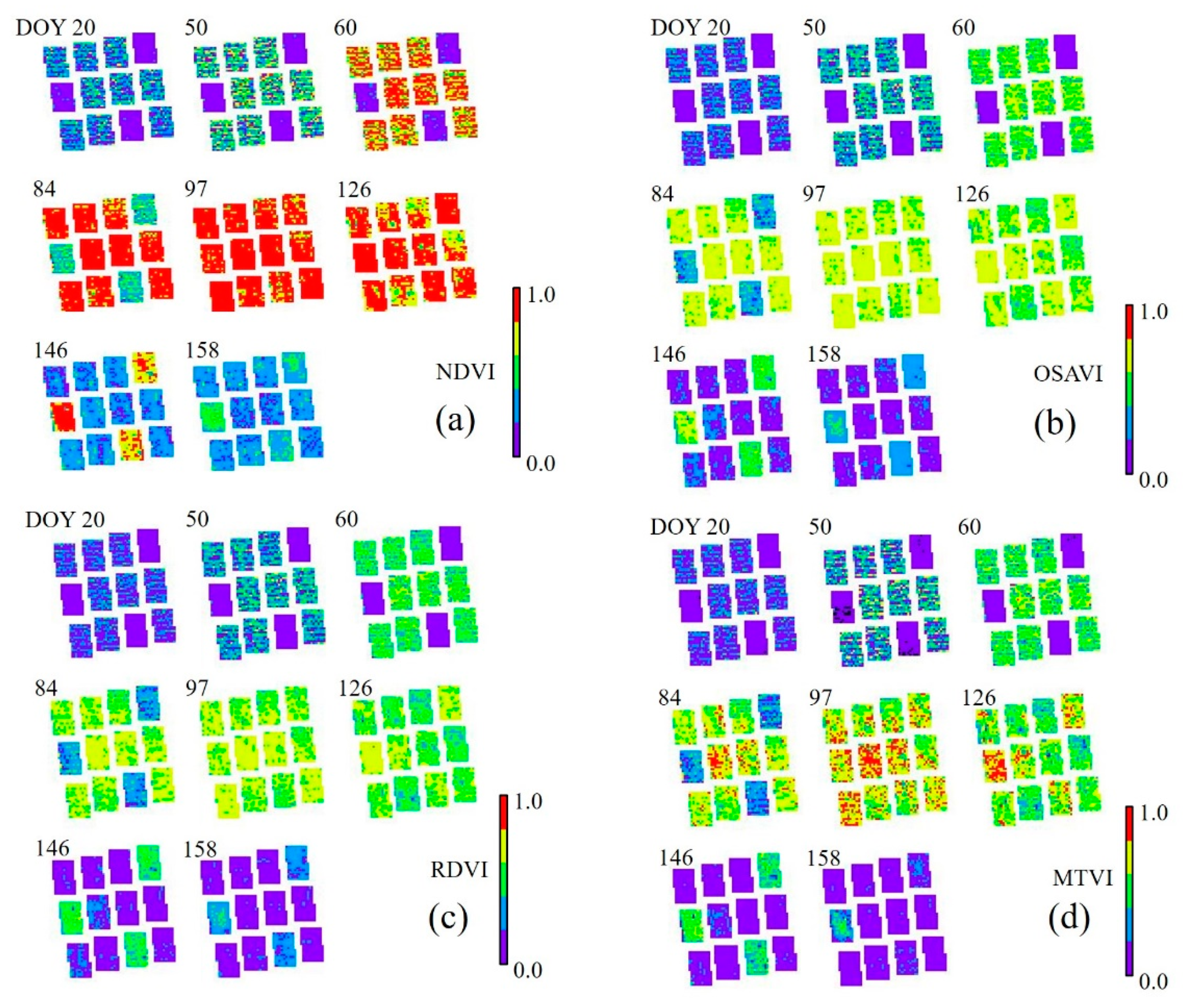
Figure A5. Variations in observed wheat vegetation indices at the Gyeongsang National University field in 2021. NDVI, normalised difference vegetation index (a), OSAVI, optimised soil-adjusted vegetation index (b), RDVI, re-normalised difference vegetation index (c), and MTVI, modified triangular vegetation index (d).
Remotesensing 14 05443 g0a5
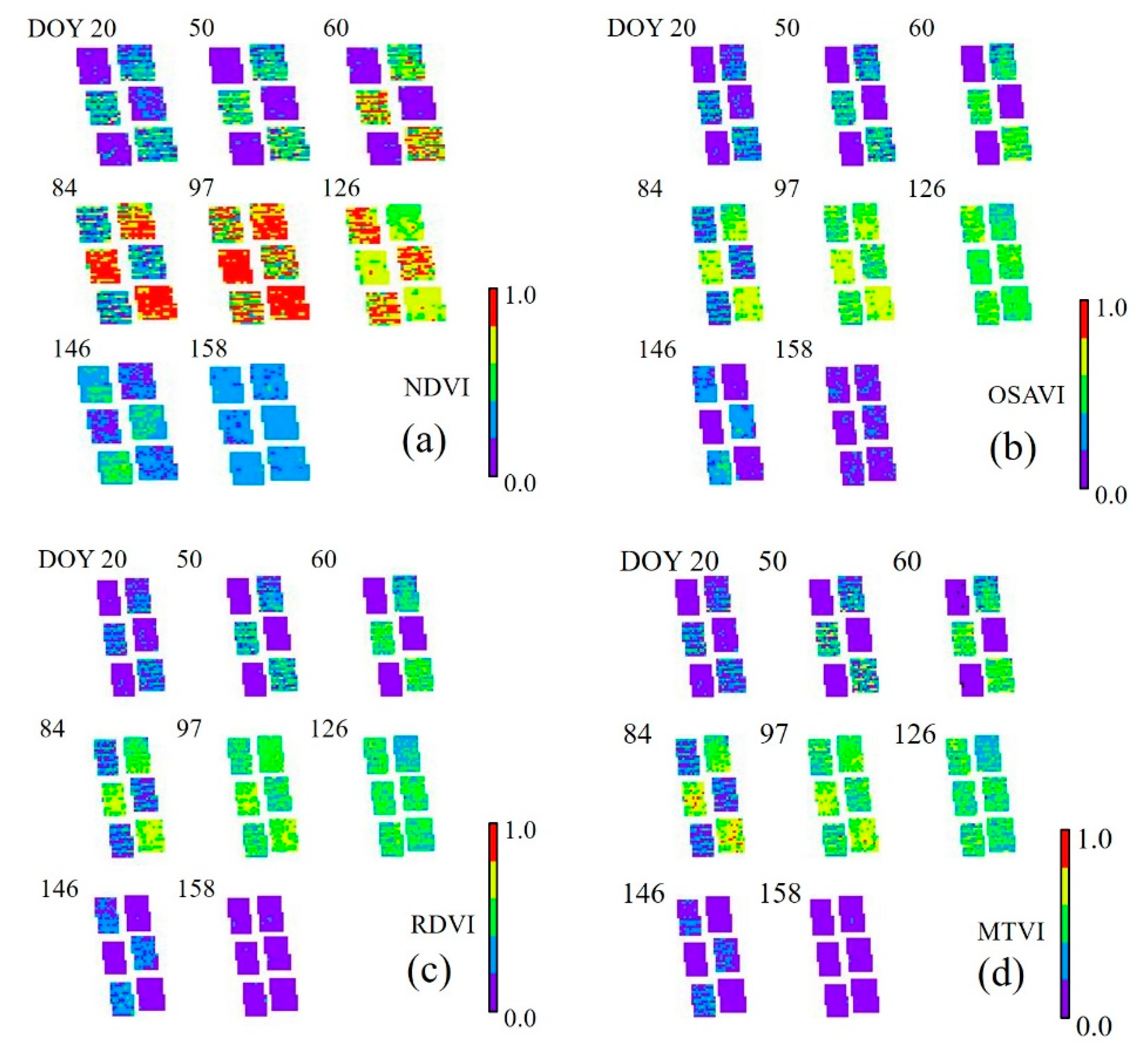
Figure A6. Variations in observed barley vegetation indices at the Gyeongsang National University field in 2021. NDVI, normalised difference vegetation index (a), OSAVI, optimised soil-adjusted vegetation index (b), RDVI, re-normalised difference vegetation index (c), and MTVI, modified triangular vegetation index (d).
Remotesensing 14 05443 g0a6

References

  1. Khaki, S.; Wang, L.; Archontoulis, S.V. A CNN-RNN framework for crop yield prediction. Front. Plant Sci. 2020, 10, 1750. [Google Scholar] [CrossRef] [PubMed]
  2. Kim, N.; Na, S.-I.; Park, C.-W.; Huh, M.; Oh, J.; Ha, K.-J.; Cho, J.; Lee, Y.-W. An artificial intelligence approach to prediction of corn yields under extreme weather conditions using satellite and meteorological data. Appl. Sci. 2020, 10, 3785. [Google Scholar] [CrossRef]
  3. Kumar, P.; Prasad, R.; Choudhary, A.; Gupta, D.K.; Mishra, V.N.; Vishwakarma, A.K.; Singh, A.K.; Srivastava, P.K. Comprehensive evaluation of soil moisture retrieval models under different crop cover types using C-band synthetic aperture radar data. Geocarto Int. 2019, 34, 1022–1041. [Google Scholar] [CrossRef]
  4. Everingham, Y.; Sexton, J.; Skocaj, D.; Inman-Bamber, G. Accurate prediction of sugarcane yield using a random forest algorithm. Agron. Sustain. Dev. 2016, 36, 27. [Google Scholar] [CrossRef] [Green Version]
  5. Feng, P.; Wang, B.; Li Liu, D.; Waters, C.; Yu, Q. Incorporating machine learning with biophysical model can improve the evaluation of climate extremes impacts on wheat yield in south-eastern Australia. Agric. For. Meteorol. 2019, 275, 100–113. [Google Scholar] [CrossRef]
  6. Shahhosseini, M.; Hu, G.; Huber, I.; Archontoulis, S.V. Coupling machine learning and crop modelling improves crop yield prediction in the US Corn Belt. Sci. Rep. 2021, 11, 1606. [Google Scholar] [CrossRef] [PubMed]
  7. Cai, Y.; Guan, K.; Nafziger, E.; Chowdhary, G.; Peng, B.; Jin, Z.; Wang, S.; Wang, S. Detecting in-season crop nitrogen stress of corn for field trials using UAV- and CubeSat-based multispectral sensing. IEEE J. Sel. Top. Appl. Earth Obs. Remote Sens. 2019, 12, 5153–5166. [Google Scholar] [CrossRef]
  8. van Klompenburg, T.; Kassahun, A.; Catal, C. Crop yield prediction using machine learning: A systematic literature review. Comput. Electron. Agric. 2020, 177, 105709. [Google Scholar] [CrossRef]
  9. Jeong, S.; Ko, J.; Yeom, J.-M. Predicting rice yield at pixel scale through synthetic use of crop and deep-learning models with satellite data in South and North Korea. Sci. Total Environ. 2022, 802, 149726. [Google Scholar] [CrossRef] [PubMed]
  10. Jeong, S.; Ko, J.; Shin, T.; Yeom, J.-m. Incorporation of machine learning and deep neural network approaches into a remote sensing-integrated crop model for the simulation of rice growth. Sci. Rep. 2022, 12, 9030. [Google Scholar] [CrossRef] [PubMed]
  11. Campbell, J.B.; Wynne, R.H. Introduction to Remote Sensing; Guilford Press: New York, NY, USA, 2011. [Google Scholar]
  12. Khanal, S.; KC, K.; Fulton, J.P.; Shearer, S.; Ozkan, E. Remote sensing in agriculture—Accomplishments, limitations, and opportunities. Remote Sens. 2020, 12, 3783. [Google Scholar] [CrossRef]
  13. Dorigo, W.A.; Zurita-Milla, R.; de Wit, A.J.W.; Brazile, J.; Singh, R.; Schaepman, M.E. A review on reflective remote sensing and data assimilation techniques for enhanced agroecosystem modelling. Int. J. Appl. Earth Obs. Geoinf. 2007, 9, 165–193. [Google Scholar] [CrossRef]
  14. Zarco-Tejada, P.J.; Ustin, S.L.; Whiting, M.L. Temporal and spatial relationships between within-field yield variability in cotton and high-spatial hyperspectral remote sensing imagery. Agron. J. 2005, 97, 641–653. [Google Scholar] [CrossRef] [Green Version]
  15. Kern, A.; Barcza, Z.; Marjanović, H.; Árendás, T.; Fodor, N.; Bónis, P.; Bognár, P.; Lichtenberger, J. Statistical modelling of crop yield in Central Europe using climate data and remote sensing vegetation indices. Agric. For. Meteorol. 2018, 260, 300–320. [Google Scholar] [CrossRef]
  16. Labus, M.P.; Nielsen, G.A.; Lawrence, R.L.; Engel, R.; Long, D.S. Wheat yield estimates using multi-temporal NDVI satellite imagery. Int. J. Remote Sens. 2002, 23, 4169–4180. [Google Scholar] [CrossRef]
  17. Delécolle, R.; Maas, S.J.; Guérif, M.; Baret, F. Remote sensing and crop production models: Present trends. ISPRS J. Photogramm. Remote Sens. 1992, 47, 145–161. [Google Scholar] [CrossRef]
  18. Becker-Reshef, I.; Vermote, E.; Lindeman, M.; Justice, C. A generalised regression-based model for forecasting winter wheat yields in Kansas and Ukraine using MODIS data. Remote Sens. Environ. 2010, 114, 1312–1323. [Google Scholar] [CrossRef]
  19. Jones, J.W.; Hoogenboom, G.; Porter, C.H.; Boote, K.J.; Batchelor, W.D.; Hunt, L.; Wilkens, P.W.; Singh, U.; Gijsman, A.J.; Ritchie, J.T. The DSSAT cropping system model. Eur. J. Agron. 2003, 18, 235–265. [Google Scholar] [CrossRef]
  20. van Diepen, C.A.; Wolf, J.; van Keulen, H.; Rappoldt, C. WOFOST: A simulation model of crop production. Soil Use Manag. 1989, 5, 16–24. [Google Scholar] [CrossRef]
  21. Cao, J.; Zhang, Z.; Tao, F.; Zhang, L.; Luo, Y.; Zhang, J.; Han, J.; Xie, J. Integrating multi-source data for rice yield prediction across China using machine learning and deep learning approaches. Agric. For. Meteorol. 2021, 297, 108275. [Google Scholar] [CrossRef]
  22. Maas, S.J. Parameterized model of gramineous crop growth: II. within-season simulation calibration. Agron. J. 1993, 85, 354–358. [Google Scholar] [CrossRef]
  23. Nguyen, V.; Jeong, S.; Ko, J.; Ng, C.; Yeom, J. Mathematical integration of remotely sensed information into a crop modelling process for mapping crop productivity. Remote Sens. 2019, 11, 2131. [Google Scholar] [CrossRef] [Green Version]
  24. Huang, J.; Gómez-Dans, J.L.; Huang, H.; Ma, H.; Wu, Q.; Lewis, P.E.; Liang, S.; Chen, Z.; Xue, J.-H.; Wu, Y.; et al. Assimilation of remote sensing into crop growth models: Current status and perspectives. Agric. For. Meteorol. 2019, 276, 107609. [Google Scholar] [CrossRef]
  25. Jin, X.; Kumar, L.; Li, Z.; Feng, H.; Xu, X.; Yang, G.; Wang, J. A review of data assimilation of remote sensing and crop models. Eur. J. Agron. 2018, 92, 141–152. [Google Scholar] [CrossRef]
  26. Shawon, A.R.; Ko, J.; Ha, B.; Jeong, S.; Kim, D.K.; Kim, H.-Y. Assessment of a proximal sensing-integrated crop model for simulation of soybean growth and yield. Remote Sens. 2020, 12, 410. [Google Scholar] [CrossRef] [Green Version]
  27. Shawon, A.R.; Ko, J.; Jeong, S.; Shin, T.; Lee, K.D.; Shim, S.I. Two-dimensional simulation of barley growth and yield using a model integrated with remote-controlled aerial imagery. Remote Sens. 2020, 12, 3766. [Google Scholar] [CrossRef]
  28. Shin, T.; Ko, J.; Jeong, S.; Shawon, A.R.; Lee, K.D.; Shim, S.I. Simulation of wheat productivity using a model integrated with proximal and remotely controlled aerial sensing information. Front. Plant Sci. 2021, 12, 649660. [Google Scholar] [CrossRef]
  29. Jeong, S.; Ko, J.; Choi, J.; Xue, W.; Yeom, J.-M. Application of an unmanned aerial system for monitoring paddy productivity using the GRAMI-rice model. Int. J. Remote Sens. 2018, 39, 2441–2462. [Google Scholar] [CrossRef]
  30. Jeong, S.; Ko, J.; Kang, M.; Yeom, J.; Ng, C.T.; Lee, S.-H.; Lee, Y.-G.; Kim, H.-Y. Geographical variations in gross primary production and evapotranspiration of paddy rice in the Korean Peninsula. Sci. Total Environ. 2020, 714, 136632. [Google Scholar] [CrossRef]
  31. Yeom, J.-M.; Jeong, S.; Deo, R.C.; Ko, J. Mapping rice area and yield in north-eastern Asia by incorporating a crop model with dense vegetation index profiles from a geostationary satellite. GIScience Remote Sens. 2021, 58, 1–27. [Google Scholar] [CrossRef]
  32. Rouse, J.W., Jr.; Haas, R.H.; Schell, J.A.; Deering, D.W. Monitoring vegetation systems in the Great Plains with ERTS. In Proceedings of the NASA Goddard Space Flight Center 3d ERTS-1 Symp., Washington, DC, USA, 1 January 1974; pp. 309–317. [Google Scholar]
  33. Rondeaux, G.; Steven, M.; Baret, F. Optimization of soil-adjusted vegetation indices. Remote Sens. Environ. 1996, 55, 95–107. [Google Scholar] [CrossRef]
  34. Haboudane, D.; Miller, J.R.; Pattey, E.; Zarco-Tejada, P.J.; Strachan, I.B. Hyperspectral vegetation indices and novel algorithms for predicting green LAI of crop canopies: Modeling and validation in the context of precision agriculture. Remote Sens. Environ. 2004, 90, 337–352. [Google Scholar] [CrossRef]
  35. Roujean, J.-L.; Breon, F.-M. Estimating PAR absorbed by vegetation from bidirectional reflectance measurements. Remote Sens. Environ. 1995, 51, 375–384. [Google Scholar] [CrossRef]
  36. Monteith, J.L. Solar radiation and productivity in tropical ecosystems. J. Appl. Ecol. 1972, 9, 747–766. [Google Scholar] [CrossRef] [Green Version]
  37. Press, W.H.; Teukolsky, S.A.; Vetterling, W.T.; Flannery, B.P. Numerical Recipes: The Art of Scientific Computing; Cambridge University Press: New York, NY, USA, 1992. [Google Scholar]
  38. Nash, J.C. Compact Numerical Methods for Computers: Linear Algebra and Function Minimisation; CRC Press: New York, NY, USA, 1990. [Google Scholar]
  39. Yeom, J.-M.; Jeong, S.; Jeong, G.; Ng, C.T.; Deo, R.C.; Ko, J. Monitoring paddy productivity in North Korea employing geostationary satellite images integrated with GRAMI-rice model. Sci. Rep. 2018, 8, 16121. [Google Scholar] [CrossRef] [Green Version]
  40. Ko, J.; Jeong, S.; Yeom, J.; Kim, H.; Ban, J.-O.; Kim, H.-Y. Simulation and mapping of rice growth and yield based on remote sensing. J. Appl. Remote Sens. 2015, 9, 096067. [Google Scholar] [CrossRef]
  41. Nash, J.E.; Sutcliffe, J.V. River flow forecasting through conceptual models part I—A discussion of principles. J. Hydrol. 1970, 10, 282–290. [Google Scholar] [CrossRef]
  42. Bui, D.T.; Tsangaratos, P.; Nguyen, V.-T.; Liem, N.V.; Trinh, P.T. Comparing the prediction performance of a Deep Learning Neural Network model with conventional machine learning models in landslide susceptibility assessment. CATENA 2020, 188, 104426. [Google Scholar] [CrossRef]
  43. Sahoo, A.K.; Pradhan, C.; Das, H. Performance evaluation of different machine learning methods and deep-learning based convolutional neural network for health decision making. In Nature Inspired Computing for Data Science; Rout, M., Rout, J.K., Das, H., Eds.; Springer: Berlin/Heidelberg, Germany, 2020; pp. 201–212. [Google Scholar]
  44. Lövenstein, H.; Rabbinge, R.; van Keulen, H. World Food Production, Textbook 2: Biophysical Factors in Agricultural Production; Wageningen University & Research: Wageningen, The Netherlands, 1992. [Google Scholar]
  45. Ahuja, L.R.; Rojas, K.W.; Hanson, J.D.; Shaffer, M.J.; Ma, L. Root Zone Water Quality Model: Modelling Management Effects on Water Quality and Crop Production; Water Resources Publications, LLC.: Highland Ranch, CO, USA, 2000. [Google Scholar]
  46. Jeong, S.; Shin, T.; Ban, J.-O.; Ko, J. Simulation of spatiotemporal variations in cotton lint yield in the Texas High Plains. Remote Sens. 2022, 14, 1421. [Google Scholar] [CrossRef]
  47. Johnson, D.M. An assessment of pre-and within-season remotely sensed variables for forecasting corn and soybean yields in the United States. Remote Sens. Environ. 2014, 141, 116–128. [Google Scholar] [CrossRef]
  48. Bolton, D.K.; Friedl, M.A. Forecasting crop yield using remotely sensed vegetation indices and crop phenology metrics. Agric. For. Meteorol. 2013, 173, 74–84. [Google Scholar] [CrossRef]
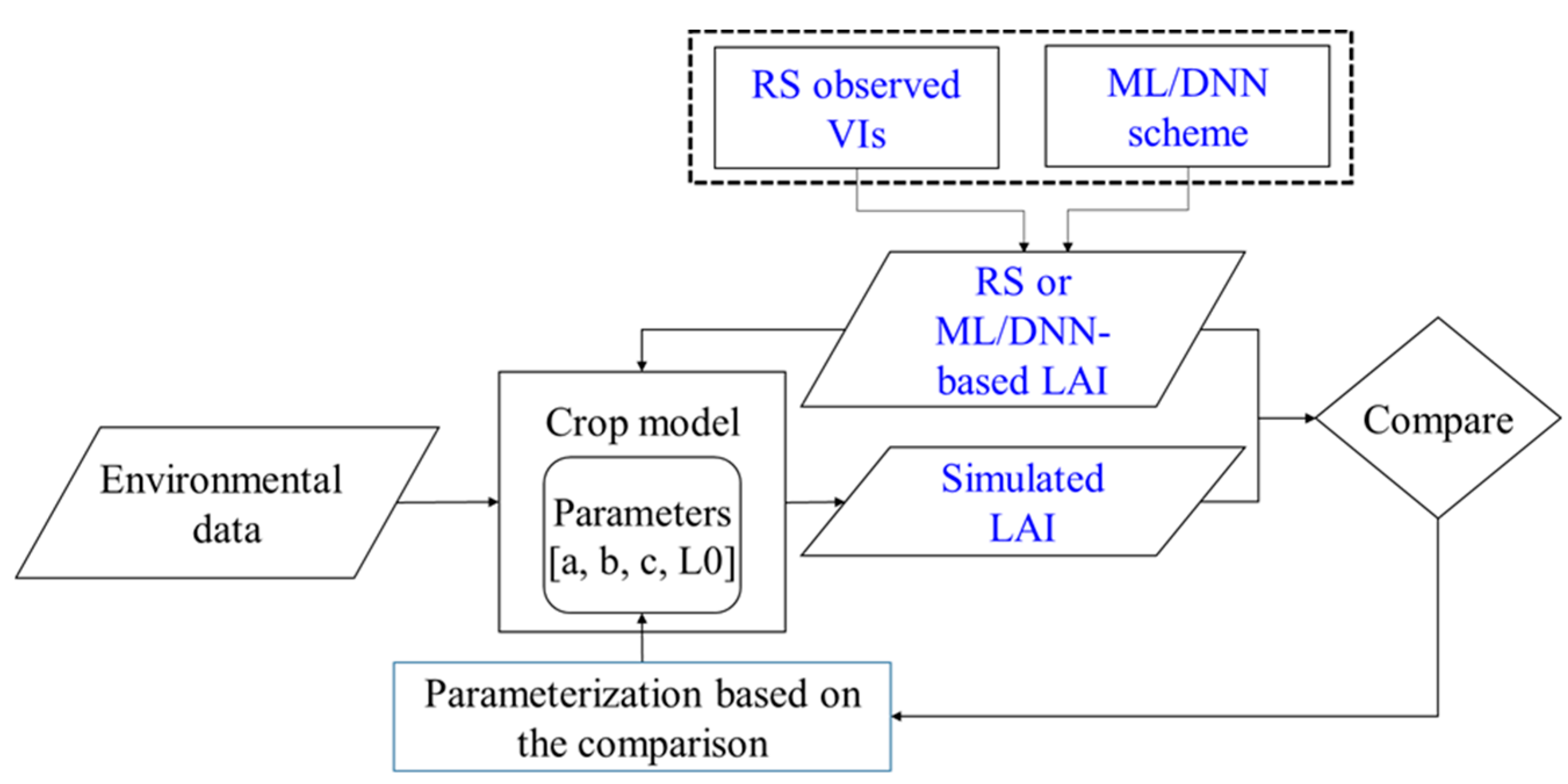
Figure 1. Schematic diagram of the process-based mathematical crop model integrated with RS-observed vegetation indices (VIs) or machine learning (ML) and DNN schemes to simulate LAI and yield. A statistical comparison between the RS or ML/DNN-based LAI and the simulated LAI values is achieved. The dotted line box represents the optional input procedure of the mathematical regression for the ML or DNN regressor to the estimated LAI. The environmental data include incident solar radiation and minimum and maximum atmospheric temperatures.
Remotesensing 14 05443 g001
Figure 2. Leaf area index (LAI) in association with four different vegetation indices of interest for barley. MTVI1, NDVI, OSDVI, and RDVI represent the modified triangular vegetation index 1, normalised difference vegetation index, optimised soil-adjusted vegetation index, and re-normalised difference vegetation index, respectively.
Remotesensing 14 05443 g002
Figure 3. Leaf area index (LAI) in association with four different vegetation indices of interest for wheat. MTVI1, NDVI, OSDVI, and RDVI represent the modified triangular vegetation index 1, normalised difference vegetation index, optimised soil-adjusted vegetation index, and re-normalised difference vegetation index, respectively.
Remotesensing 14 05443 g003
Figure 4. Comparisons between simulated (Sim) and observed (Obs) leaf area index (LAI) values for wheat by (a) Gradient Boost and (b) deep neural network regression models.
Remotesensing 14 05443 g004
Figure 5. Comparisons between simulated (Sim) and observed (Obs) LAI values for barley by (a) Gradient Boost and (b) deep neural network (DNN) regression models.
Remotesensing 14 05443 g005
Figure 6. Simulated (Sim) versus observed (Obs) leaf area index (LAI) values of wheat at the Gyeongsang National University field, Jinju, South Gyeongsang Province, Republic of Korea: (a) autumn-sown with nitrogen (N) treatments of 40% (40 kg ha−1) at seeding, 30% (30 kg ha−1) at rejuvenation, and 0% (0 kg ha−1) at early reproduction (N40-30-0); (b) autumn-sown N40-30-30, (c) autumn-sown N40-30-60, and (d) spring-sown N40-30-30.
Remotesensing 14 05443 g006
Figure 7. Simulated (Sim) versus observed (Obs) leaf area index (LAI) values of barley at the Gyeongsang National University field: (a) autumn-sown with nitrogen (N) treatments of 40% (32 kg ha−1) at seeding, 30% (24 kg ha−1) at rejuvenation, and 30% (24 kg ha−1) at early reproduction (N40-30-30) and (b) spring-sown N40-30-30.
Remotesensing 14 05443 g007
Figure 8. The plots show 2D variations in simulated wheat yield (a) and the corresponding box and whisker plots (b) at the Gyeongsang National University field in 2021. AN1 = autumn-sown with nitrogen (N) treatments of 40% (40 kg ha−1) at seeding, 30% (30 kg ha−1) at rejuvenation, and 0% (0 kg ha−1) at early reproduction (N40-30-0); AN2 = autumn-sown N40-30-30; AN3 = autumn-sown N40-30-60; SN = spring-sown N40-30-30. The numbers adjacent to the dash symbols represent experimental blocks. Error bars and boxes represent the yield data’s 10th, 25th, 75th, and 90th percentiles, presenting the median (solid line) and mean (×).
Remotesensing 14 05443 g008
Figure 9. The plots show 2D variations in simulated barley yield (a) and the corresponding box and whisker plots (b) at the Gyeongsang National University field in 2021. AN = autumn-sown with nitrogen (N) treatments of 40% (32 kg ha−1) at seeding, 30% (24 kg ha−1) at rejuvenation, and 30% (24 kg ha−1) at early reproduction (N40-30-30); SN = spring-sown N40-30-30. The numbers adjacent to the dash symbols represent experimental blocks. Error bars and boxes represent the yield data’s 10th, 25th, 75th, and 90th percentiles, presenting the median (solid line) and mean (×).
Remotesensing 14 05443 g009
Table 1. Records of seeding, harvest, leaf area index (LAI) measurements, unmanned aerial system (UAS) image acquisitions events, and daily mean weather conditions during the barley and wheat growing seasons from 2018 to 2021.
DivisionUnit 2018201920202021
SeedingDD/MM/YY30/10/1705/11/18
(18/02/19)
30/10/19
(20/02/20)
30/10/20
(19/02/21)
HarvestDD/MM/YY25/06/1810/06/1909/06/2007/06/21
LAI
measurement
DOY87, 101, 115, 130, 14468, 81, 102, 111, 14562, 79, 93, 107, 129, 14359, 69, 84, 97, 111, 127
UAS image
acquisition
DOY87, 101, 115, 130, 144, 15853, 67, 81, 102, 123, 14475, 85, 99, 107, 120, 134, 14320, 50, 60, 84, 97, 126, 146, 158
Temperature°C8.798.2815.9615.55
Solar radiationMJ m−2 d−111.8113.1115.8114.71
Precipitationmm d12.961.952.602.05
DD/MM/YY and DOY are two-digit numbers representing ‘date/month/year’ and ‘day of year’. The values in the parentheses represent spring-seeded dates.
Table 2. Training and test scores for the leaf area index estimation analyses of barley and wheat in relation to remote sensing data using ten machine learning regression models.
RegressorBarelyWheat
TrainingTestTrainingTest
Extra Trees0.9990.7780.9990.681
Gradient Boosting0.9720.8140.9910.685
HGB0.9180.7900.5680.335
Lasso0.8430.7870.6120.492
LGBM0.9150.7730.5420.344
Polynomial Linear0.8720.7590.7140.455
Random Forest0.9750.8030.9470.631
Ridge0.8720.7610.6090.502
Support Vector0.8630.7710.7330.525
XGB0.9990.7820.9990.554
HGB, LGBM, and XGB stand for Histogram-based Gradient Boosting, Light Gradient Boosting Machine, and Extreme Gradient Boosting models.
Table 3. Observed (Obs) versus simulated (Sim) LAI values of barley and wheat according to absolute mean error (MAE), root mean squared deviation (RMSD), and Nash–Sutcliffe model efficiency (ME) for the Gradient Boost (GB) and deep neural network (DNN) regression models.
CropGBDNN
SimObsMAERMSDMESimObsMAERMSDME
--------------- m2 m−2 -------------None-------------- m2 m−2 --------------None
Barley3.32 ± 1.923.47 ± 2.020.490.670.893.45 ± 1.843.32 ± 2.100.620.820.85
Wheat2.93 ± 0.752.81 ± 0.970.590.710.452.93 ± 0.643.07 ± 0.840.540.640.41
Table 4. Observed versus simulated wheat grain yields for the different treatments in terms of the p-value shown by the t-test, the mean absolute error (MAE), the root mean squared deviation (RMSD), and normalised Nash–Sutcliffe model efficiency (NME).
TreatmentYield (mean ± 1 SD)pMAERMSDNME
SimulatedObserved
--------- tonne ha−1 ---------unitless---- tonne ha−1 ----unitless
AN14.538 ± 0.2374.415 ± 1.0490.8500.6590.7541.000
AN25.611 ± 0.2065.920 ± 0.7660.5370.5460.5940.995
AN37.221 ± 0.2327.627 ± 1.5120.6690.8401.1290.998
SN4.308 ± 0.5254.272 ± 0.2850.9220.5430.5920.790
AN1 = autumn-sown with nitrogen (N) treatments of 40 kg ha−1 at seeding, 30 kg ha−1 at rejuvenation, and 0 kg ha−1 at early reproduction (N40-30-0); AN2 = autumn-sown N40-30-30; AN3 = autumn-sown N40-30-60; SN = spring-sown N40-30-30. The numbers next to each dash symbol represent experimental blocks.
Table 5. Observed versus simulated barley grain yields for the different treatments in terms of the p-value shown by the t-test, the mean absolute error (MAE), the root mean squared deviation (RMSD), and normalised Nash–Sutcliffe model efficiency (NME).
TreatmentYield (mean ± 1 SD)pMAERMSDNME
SimulatedObserved
--------- tonne ha−1 ---------unitless---- tonne ha−1 ----unitless
AN4.415 ± 0.7794.276 ± 0.6590.8250.5190.5590.989
SN3.790 ± 0.0534.001 ± 0.0490.0070.2110.2120.000
AN = autumn-sown with nitrogen (N) treatments of 40% (32 kg ha−1) at seeding, 30% (24 kg ha−1) at rejuvenation, and 30% (24 kg ha−1) at early reproduction (N40-30-30) and SN = spring-sown N40-30-30.
Publisher’s Note: MDPI stays neutral with regard to jurisdictional claims in published maps and institutional affiliations.