Simulation of Spatiotemporal Variations in Cotton Lint Yield in the Texas High Plains

Abstract

This study aimed to simulate the spatiotemporal variation in cotton (Gossypium hirsutum L.) growth and lint yield using a remote sensing-integrated crop model (RSCM) for cotton. The developed modeling scheme incorporated proximal sensing data and satellite imagery. We formulated this model and evaluated its accuracy using field datasets obtained in Lamesa in 1999, Halfway in 2002 and 2004, and Lubbock in 2003–2005 in the Texas High Plains in the USA. We found that RSCM cotton could reproduce the cotton leaf area index and lint yield across different locations and irrigation systems with a statistically significant degree of accuracy. RSCM cotton was also used to simulate cotton lint yield for the field circles in Halfway. The RSCM system could accurately reproduce the spatiotemporal variations in cotton lint yield when integrated with satellite images. From the results of this study, we predict that the proposed crop-modeling approach will be applicable for the practical monitoring of cotton growth and productivity by farmers. Furthermore, a user can operate the modeling system with minimal input data, owing to the integration of proximal and remote sensing information.

1. Introduction

Cotton is a perennial warm-season crop and the most common material used in textiles [1]. The top cotton producing countries include China, India, and the United States (https://www.statista.com/statistics/263055/, accessed on 30 December 2021). Within the United States, Texas produces the greatest share of cotton. There are more than 2 million ha of cotton farms in Texas, which account for approximately 50% of the cotton fields and 40% of the total production in the United States (https://www.nass.usda.gov/, accessed on 30 December 2021). Therefore, agricultural sector stakeholders, policymakers, and researchers are interested in gathering pre-, post-, and mid-season productivity information for these cotton-producing regions. Developing an effective monitoring system is necessary for gathering this information.

Remote sensing is a valuable technique used to measure crop growth and development conditions, which are affected by geographic and spatial variability during crop growing seasons [2]. It helps obtain detailed information about crop growth conditions from a region of interest. Crop growth conditions and yields can be estimated by analyzing the relationship between crop growth variables and remote sensing information [3,4]. For example, many endeavors have been made to estimate crop yields based on optical remote sensing data [5,6]. Such empirical modeling approaches are practical and suitable for determining growth conditions and productivity in specific regions of interest. However, these empirical modeling methodologies are not sufficient for explaining the growth and development processes or their influences on productivity [7,8]. In addition, it is not possible to obtain the necessary information from a continuous source when using most satellite images because of the restricted revisit time of the fields of interest or unfavorable environmental conditions [9].

A crop model integrated with remote sensing information can be effectively applied to model crop growth and development, and thus to monitor productivity [10]. Most mathematical crop models are beneficial for describing seasonal variations in crop growth and development [11,12]. However, they are limited in providing spatiotemporal projections based on crop modeling, owing to either the restricted availability of input parameters and variables or high input requirements. While remote sensing techniques are suitable for providing two-dimensional images of crop conditions [13,14], these approaches have limitations in generating information regarding temporal variations in crop growth and performance [10]. As a result, there have been substantial efforts to integrate remote sensing information into crop models to strengthen their advantages and compensate for their weaknesses [10,15,16,17]. One such effort is developing a remote sensing-integrated crop model (RSCM) [10,18]. RSCM (previously GRAMI) was designed to model gramineous crops (such as maize, sorghum, and wheat), using simple weather variables and remote sensing data. The RSCM technique has been applied to various aspects of crop production monitoring, from proximal sensing to remote sensing, using remote-controlled aerial systems and satellite platforms [19,20].

An earlier version of the RSCM for simulating cotton growth [21] was developed based on the GRAMI model [22,23]. This modeling approach integrated proximal sensing data and was also applied to simulate cotton growth and yield under conditions of poor irrigation [24]. However, no further efforts have been made to employ an integrated system using other established remote sensing platforms such as airborne or satellite sensing. Therefore, the objective of the present study was to improve the previous cotton modeling approach with integrated proximal sensing data and to investigate the practical monitoring capabilities of integrating satellite-based remote sensing data.

2. Materials and Methods

2.1. Study Site Description

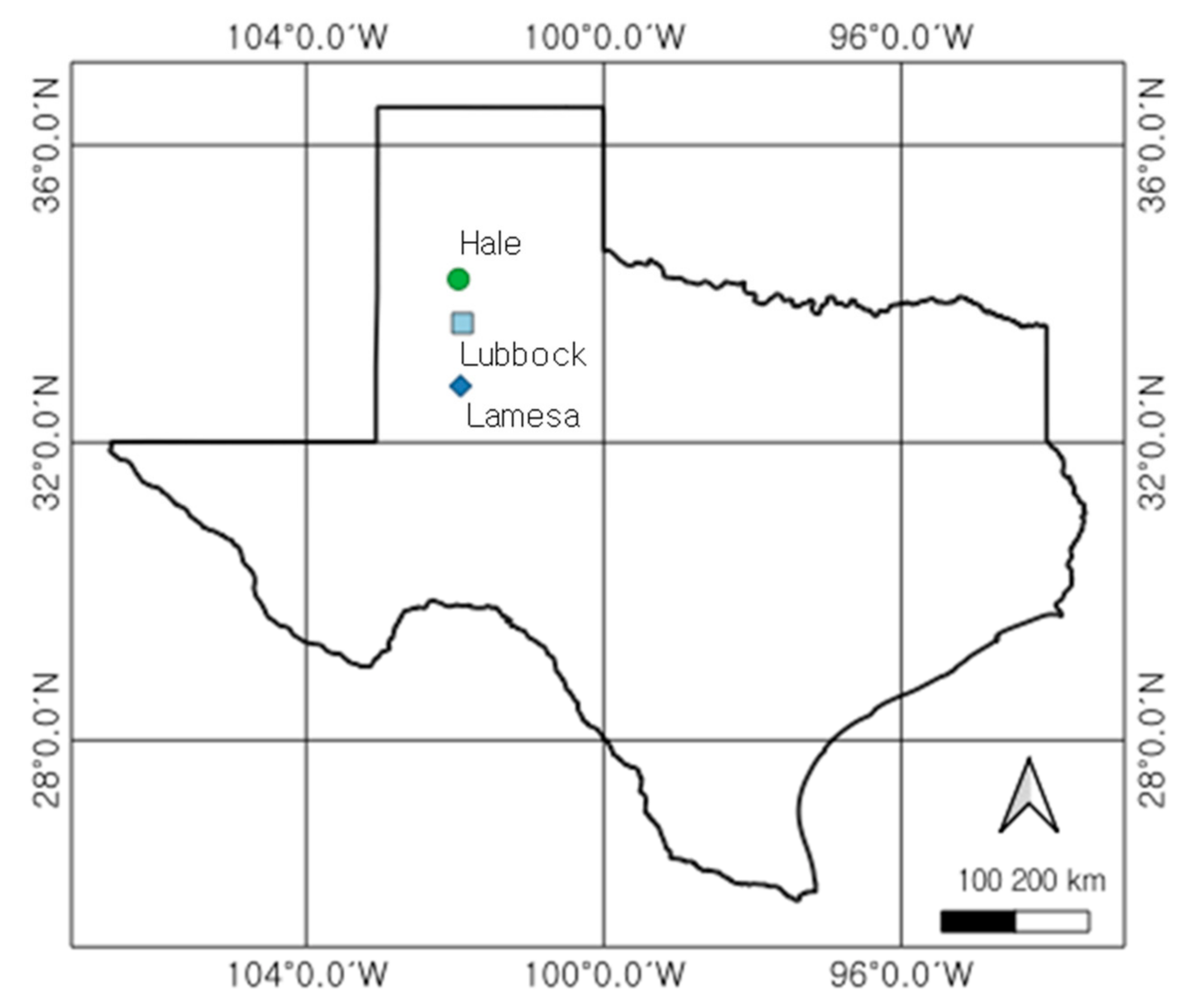
The study field sites were in Hale, Lamesa, and Lubbock, Texas, USA (Figure 1). These study locations are located in the Southern Great Plains region, which experiences a continental climate with low precipitation and humidity, high winds, and sudden temperature changes (https://www.britannica.com/place/Great-Plains, accessed on 14 January 2022). As a result, the southern plains experience cold winters and warm summers. The average rainfall is 380 to 640 mm, but there are substantial yearly variations in both total and seasonal rainfall.

The High Plains region of Texas, where the study sites were located, produces 64% of the state’s cotton (https://www.nass.usda.gov/Data_and_Statistics/, accessed on 24 January 2022). Fifty percent of the cotton in this region requires irrigation. Additionally, the area’s warm days and cool nights, as well as its loam and sandy soil types, mean that soil and water conservation processes are crucial in this region.

Figure 1. Map of study field locations in Hale, Lubbock, and Lamesa counties, Texas, USA.

Figure 1. Map of study field locations in Hale, Lubbock, and Lamesa counties, Texas, USA.

2.2. Cotton Data

The field datasets of this study were obtained from commercial cotton farm fields #26, #28, and #30 near Halfway in Hale, a Plant Stress and Water Conservation Laboratory (PSWCL) field in Lubbock, and a Texas A&M University Agricultural Research (TAMUAR) farm near Lamesa, Texas, USA (

Table 1. Summarized information on the study fields and irrigation methods.

Field Division	Location	Size (ha)	Field Shape	Soil Type	Irrigation Method
#26	Halfway	50	Circle	Brownfield fine sand	LEPA
#28	Halfway	50	Circle	Brownfield fine sand	LEPA
#30	Halfway	50	Circle	Brownfield fine sand	LEPA
TAMUAR	Lamesa	45	Circle	Amarillo fine sandy loam	LEPA
PSWCL	Lubbock	5	Rectangle	Amarillo fine sandy loam	Subsurface drip

TAMUAR, PSWCL, and LEPA stand for Texas A&M University Agricultural Research, Plant Stress and Water Conservation Laboratory, and low-energy precision application.

). Halfway fields #26 (34°2′41″ N, 102°2′18″ W), #28 (34°4′6″ N, 102°11′10″ W), and #30 (34°4′5″ N, 102°11′8″ W) were circular and approximately 50 ha in size. These fields had Brownfield fine sands [21,25]. The TAMUAR farm (32°16′ N, 101°56′ W) was also circular, with Amarillo fine sandy loam [21]. Finally, the PSWCL field (33°35′38″ N, 101°54′04″ W) had three irrigation treatments in 2003 and 2004 and four irrigation treatments in 2005 with 165 × 10 m study plots at three replications with Amarillo fine sandy loam [24].

The cotton cultivar Paymaster 2326 BG/RR (Delta and Pine Land Co., Scott, MS, USA) was typically seeded in mid-May from 2000 to 2003, with a row spacing of 1.0 m in Halfway fields #26, #28, and #30. In the TAMUAR farm, Paymaster 2326 RR was planted with a row spacing of 1.0 m on 10 May 1999 and 28 May 2001. Paymaster 2326 BG/RR was sown in north–south rows spaced 1.0 m apart on 13 May for 4 years (2002–2005) in the PSWCL field. Deficit irrigation was applied using a low-energy precision application system at Halfway and TAMUAR. The irrigation application quantities varied over the years, depending on the precipitation amounts received during the growing seasons. Irrigation treatments at PSWCL were established using a subsurface drip irrigation system with different application levels. Irrigation water was applied at 2, 4, 6, and 8 mm per day in 2005. Then, irrigation was conducted at 5.5, 6.5, and 8.5 h intervals in 2003 and 2004. Field cultivation and management were performed based on general cotton production guides from Texas A&M AgriLife Research and Extension Center (https://lubbock.tamu.edu/programs/crops/cotton/general-production/, accessed on 25 January 2022).

Leaf area was measured using an LI-3100 leaf area meter (LI-COR Inc., Lincoln, NE, USA) in the laboratory, using ten representative plant samples. Plants were sampled in Halfway fields #26, #28, and #30 and at the TAMUAR farm every two weeks. Plant samples were collected from PSWCL on the following days of the year: 171, 191, 210, 226, and 254 in 2002; 174, 190, 224, and 266 in 2003; 173, 194, 229, and 264 in 2004; and 187, 206, 243, and 296 in 2015. The leaf area index (LAI) was calculated as the leaf area per plant, divided by ground area per plant. The cotton lint yield was measured at the end of the growing season by hand-harvesting randomly chosen zones from each plot (or by harvesting rows using a cotton stripper in the case of the TAMUAR farm). Additionally, the cotton lint yield for each year from the entire #26, #28, and #30 fields was measured using a cotton stripper equipped with optical yield monitors (Model AG700, AGRIplan, Stow, MA, USA) and a differential global positioning system (DGPS) with sub-meter accuracy [26]. These yield data were calibrated and composited into a single yield data file and combined into 30 × 30 m pixels using the Interpolation to Raster routine (inverse distance weighting to the power of two) of Spatial Analyst in ArcMap (ESRI, Redlands, CA, USA). The cotton yield pixel files were then georeferenced to the Universal Transverse Mercator (UTM) Zone 13N projection and the North American Datum of 1983 (NAD83).

Weather data for the field sites at Halfway and Lubbock were obtained from the Texas ET Network (https://texaset.tamu.edu/, accessed on 5 March 2022) and the PSWC weather stations respectively. Meanwhile, weather data at Lamesa were collected using a standard Campbell Scientific meteorological station (Campbell Scientific Inc., Logan, UT, USA).

2.3. Proximal Sensing and Satellite Data

The cotton canopy reflectance at PSWCL from 2003 to 2005 was measured using a handheld multispectral radiometer (CROPSCAN Inc., Rochester, MN, USA). The proximal radiometer uses 16 bands to measure incident and reflected solar radiation with a 28° field of view. The center wavebands (CWB) and bandwidths (BW) for the three filters used in this study were CWB 460 nm with BW 10.0 nm, CWB 660 nm with BW 10.0 nm, and CWB 800 nm with BW 65.0 nm. Radiometer calibration was performed according to the one-point calibration procedure, using a white reference panel to compare down sensor readings and measure reflectance. The field measurement, including LAI measurement, was periodically conducted at 2 m vertically above objective zones. This measurement condition was determined to represent the cotton canopy reflectance in the field. The canopy reflectance was measured five times between 1100 and 1300 h CDT on clear days at three distinct spots for each experimental plot.

The satellite image data were obtained from Landsat-5 TM and Landsat-7 TM (https://www.usgs.gov/landsat-missions, accessed on 1 February 2022) during the cotton growing seasons from 2000 to 2003 and georeferenced to the UTM World Geodetic Survey 1984 (WGS84), Zone 14 [26]. The satellite data were radiometrically normalized so that the reflectance of different bands on different dates over the 4 years were consistent [27]. An area of interest (AOI) comprising fields #26, #28, and #30 was established for each satellite image. The AOI’s normalized difference vegetation index (NDVI) was calculated using the Transform process in ENVI software (Geospatial Solutions, Inc., Broomfield, CO, USA). NDVI image data were exported as ASCII format grid data and then imported to ArcToolbox (ESRI, Redlands, CA, USA). Next, the ASCII text grid files were converted to floating raster grids and projected to UTM Zone 13 NAD83, before being imported to ArcMap (ESRI, Redlands, CA, USA). Finally, the grid data were carefully georeferenced to ensure an accurate overlay of grid images. Landsat image grids were converted to polygons and then superimposed on the 4 m pixels with data on cotton lint yield.

2.4. Model Calculation and Evaluation

The RSCM for cotton created in this study was a simple crop model that adopted a radiation use efficiency (RUE) approach [28], simulating crop growth and lint yield (Figure 2a). It was integrated with proximal and remote sensing data based on specific crop growth parameters using a mathematical optimization procedure (Figure 2b), which is further explained following this section’s cotton growth modeling description. RSCM reproduces canopy growth and development using four mathematical calculations that incorporate growth-specific coefficients (

Table A1. Parameters for RSCM cotton simulation used in this study.

Parameter	Symbol or Acronym	Unit	Value
Radiation use efficiency	ε	g MJ−1	3.49
Light extinction coefficient	k	-	0.9
Specific leaf area	S	m2 g−1	0.01
Base temperature	Tb	°C	15.6
Leaf area index at transplanting	L0	m2 m−2	0.02
Partitioning parameter A	a	-	0.1
Partitioning parameter B	b	-	0.00125
Leaf senescence parameter	c	-	0.00125
Lint partitioning coefficient A	Pa	-	2
Lint partitioning coefficient B	Pb	-	3

). These coefficients include RUE, specific leaf area (SLA), light extinction coefficient (k), base temperature, and leaf partition and senescence coefficients. This modeling scheme used the same cotton growth-specific parameters determined by Ko et al. [21].

The four calculations used for cotton growth modeling (Figure 2a) take into account (a) buildup of growing degree-days (GDD), (b) solar radiation absorption in LAI, (c) daily production of above-ground dry mass (AGDM) by photosynthesis, and (d) LAI partitioning or senescence as calculated by the formula below. First, daily GDD (ΔD) was determined using the following equation.

ΔD = Max [T − T_b, 0]

(1)

where T and T_b are daily mean temperature and the base temperature of cotton, respectively. The daily production of AGDM (ΔM) and daily total intercepted PAR above the canopy (Q) were estimated using the following calculations:

ΔM = ε × Q,
Q = β × R × (1 − exp (−k × LAI))

(2)

where ε, β, R, and k represent RUE, the fractional constant (0.45) of solar radiation (β) used to calculate PAR [29], daily solar radiation, and the light extinction coefficient, respectively. The daily increase in LAI (ΔL) was calculated using the following formula:

ΔL = ΔM × P1 × S,
P1 = Max [1 – a × exp (b × D), 0]

(3)

where P1 and S represent the fraction of ΔM attributed to new leaves and specific leaf area, respectively. P1 is calculated using the above formula, where a and b are two coefficients that define the magnitude and shape, respectively, of the leaf partitioning process, and D is the accumulated GDD. The leaf senescence (L_s) coefficient used in the model was determined using the following formula:

L_s = c × (∆R_m − ∆M),
∆R_m = f_m × M

(4)

where c is a coefficient that defines the magnitude of the leaf senescence function, ∆R_m is the maintenance respiration function needed for conversion to biomass, M is the AGDM, and f_m is the maintenance respiration coefficient. The f_m value was calculated theoretically as ~1.5% of the current dry weight of a crop. The LAI typically starts to senesce after reaching a maximum value.

The cotton lint yield (ΔY) was partitioned from the fraction of ΔM to cotton lint using a dimensionless lint-partitioning function (P2).

ΔY = P2 × ΔM,
P2 = Max [1 – a × exp (b × f_GD), 0],
f_GD = GDD_pm − (P_a × GDD_m)/(GDD_m − GDD_r/P_b)

(5)

where f_GD is the lint-partitioning factor based on the cumulative G.D.D. In the f_GD function, GDD_pm, GDD_m, and GDD_r represent G.D.D.s at potential maturity, actual maturity, and reproduction, respectively, and P_a and P_b are lint partitioning coefficients. The lint yield partitioning function described earlier [21] can also be used in this context. All parameters applied in this study are listed in Table A1.

RSCM can adapt the model parameters and initial conditions to modify the crop growth variables. Mid-season calibration procedures are typically used to adjust the model approach based on the simulation and observation of readily available crop state variables of LAI or vegetation indices (VIs) [10]. The mathematical agreement between the simulated and observed LAIs is typically achieved using POWELL optimization [30] or Quasi-Newton minimization calculation [31]. Following this adjustment, all parameters was calibrated to ensure agreement between the simulations and observations. The updated RSCM system also employed this mid-season calibration procedure to input the proximal or remote sensing data (Figure 2b). This mathematical procedure optimizes the simulated and observed LAIs using the model parameters (L₀, a, b, and c) that describe the cotton canopy growth processes. As an example, the combined model parameters used for this evaluation at different locations are listed in

Table A2. Initial leaf area index (L₀), leaf partitioning and senescence (a, b, and c) parameters combined after the mid-season calibration of the remote sensing-integrated cotton model. Measurements were taken in fields #26, #28, and #33 in Halfway (HW), Texas; the Texas A&M University Agricultural Research (TAMUAR) farm near Lamesa; and the Plant Stress and Water Conservation Laboratory (PSWCL) in Lubbock of the Texas High Plains region, USA.

Field Location	Year	Cultivar	L0	a	b	c
#26, HW	2002	Paymaster 2326 BG/RR	0.00022	0.2607	0.0014	0.0185
#28, HW	2002	Paymaster 2326 BG/RR	0.00026	0.3338	0.0012	0.0408
#33, HW	2002	Paymaster 2326 BG/RR	0.00041	0.3515	0.0011	0.0429
TAMUAR	1999	Paymaster 2326 RR	0.00228	0.4821	0.0007	0.0416
TAMUAR	2001	Paymaster 2326 RR	0.00028	0.0901	0.0022	0.0086
PSWCL	2002	Paymaster 2326 BG/RR	0.01528	0.3856	0.0012	0.0002
PSWCL	2004	Paymaster 2326 BG/RR	0.01939	0.4529	0.0008	0.0223

. This mid-season calibration procedure was accomplished by incorporating observed values into the model using the mathematical approach described above to mitigate the uncertainties in crop modeling induced by possible inaccuracies or the inaccessibility of state variables such as VIs or LAI.

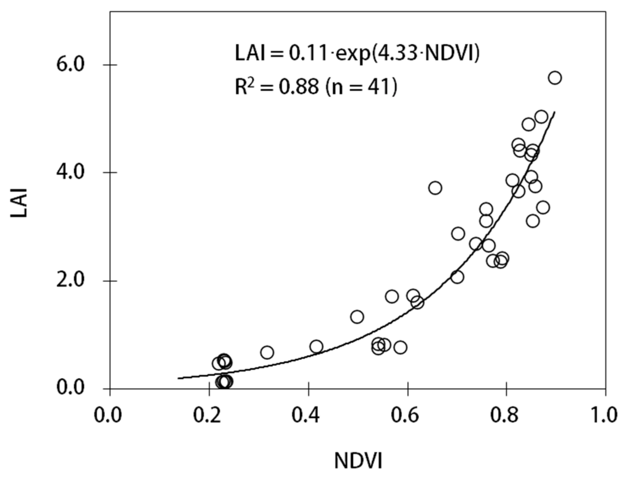
In this study, the observed LAI values for RSCM cotton simulation application for fields #26 and #28 over four years (2000–2003) were extrapolated using the parameters from the exponential relationship between LAI and NDVI (Figure 3). We assumed that the LAI and NDVI relationships at the proposed cotton fields were consistent with the experimental data obtained at PSWCL over three years (2003–2005). This hypothesis was made considering that all the cultivars planted in the study were similar to upland cotton, which should allow limited genetic variation. In addition, all the cotton cultivars were grown and cultivated in the same High Plains region environment.

Four statistical indices were employed to evaluate the performance of the RSCM cotton system: a p-value calculated using the two-sample t-test, mean absolute error (MAE), root mean square error (RMSE), and Nash–Sutcliffe model efficiency (NSME) [32]. The MAE, RMSE, and NSME were determined using the following equations.

$$\mathrm{MAE}=\frac{{{\displaystyle \sum }}_{i=1}^n\left|S_i-O_i\right|}{n}$$

(6)

$$\mathrm{RMSE}=\sqrt{\frac{1}{n}{{\displaystyle \sum }}_{i=1}^n{\left(S_i-O_i\right)}^2}$$

(7)

$$\mathrm{NSME}=1-\frac{{{\displaystyle \sum }}_{i=1}^n{\left(S_i-O_i\right)}^2}{{{\displaystyle \sum }}_{i=1}^n{\left(O_i-O_m\right)}^2}$$

(8)

where n, S_i, O_i, and O_m represent the total number of observations, the simulated value, the observed value, and the mean observed value, respectively. NSME can range from −∞ values to one. NSME values closer to one indicate more consistency and reliability, and values less than zero indicate poor reliability.

3. Results

3.1. Model Evaluation

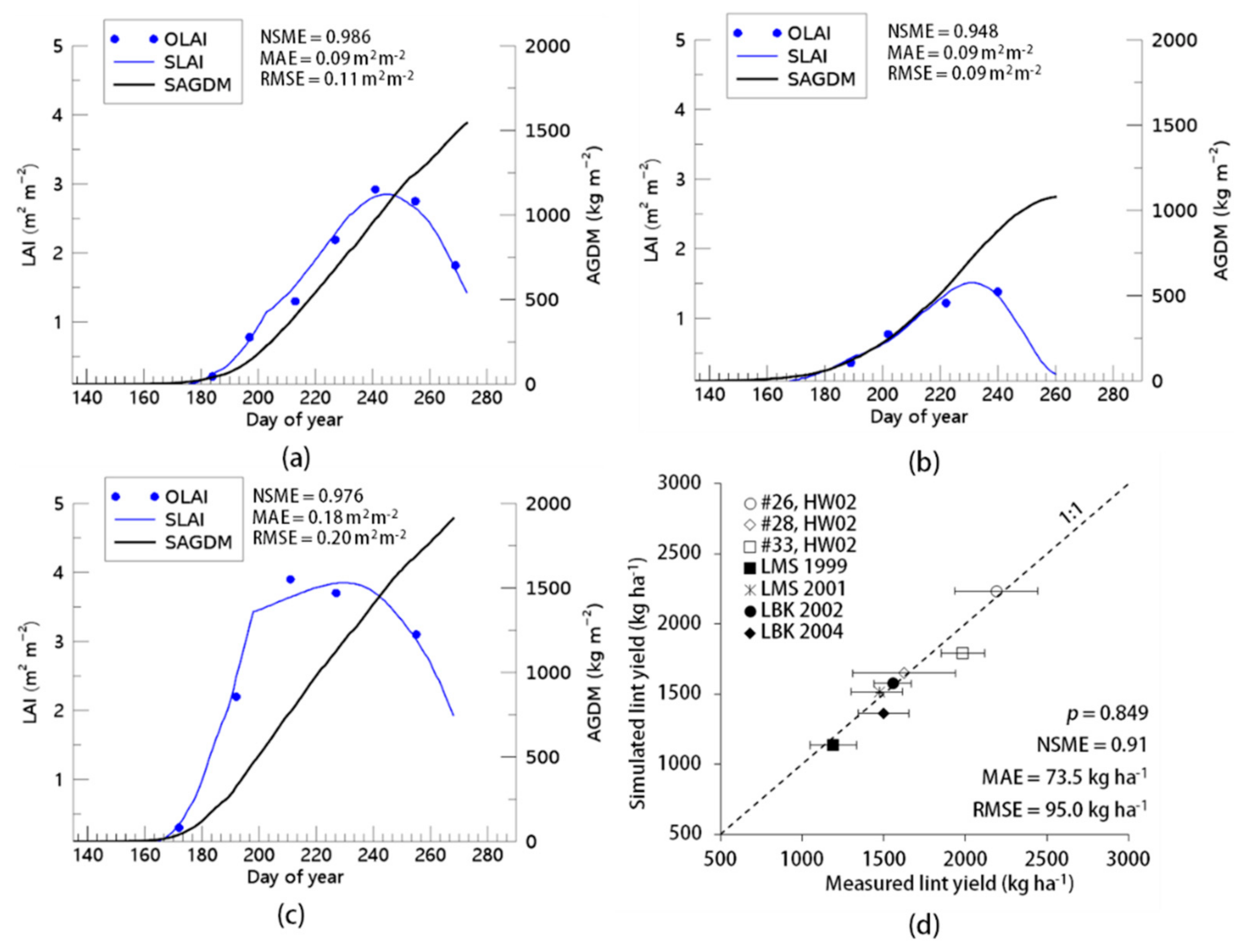
The simulated LAI values agreed with the observed LAI values to a statistically significant degree for the datasets obtained at all locations (Figure 4). For example, NSME, MAE, and RMSE were 0.986, 0.09 m² m⁻², and 0.11 m² m⁻², respectively, at Halfway field #26; 0.948, 0.09 m² m⁻², and 0.09 m² m⁻², respectively, at the Lamesa field in 1999; and 0.976, 0.18 m² m⁻², and 0.20 m² m⁻², respectively, at the Lubbock field in 2002. The simulated lint yields agreed with the measured lint yields with a p-value of 0.849 calculated by a two-sample t-test, an NSME of 0.91, an MAE of 73.5 kg ha⁻¹, and an RMSE of 95.0 kg ha⁻¹.

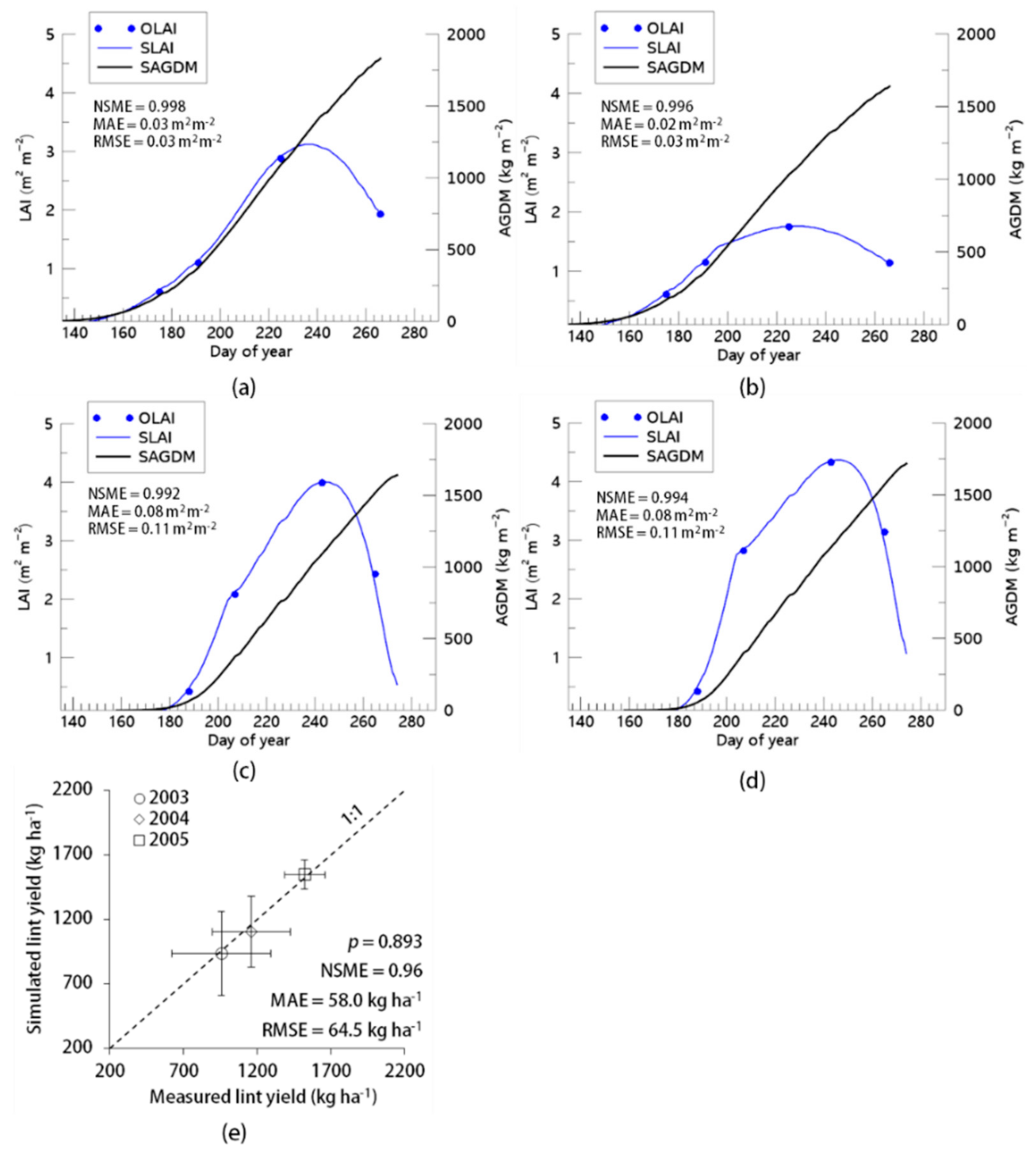
We also generated LAI observation data estimated from proximal sensing at the PSWCL field under different irrigation conditions. These were extrapolated from the LAI and NDVI relationship data (Figure 3). The simulated LAI values agreed with the observed LAI values to a statistically significant degree (Figure 5 and Figure A1) for all locations. For example, NSME, MAE, and RMSE were 0.999, 0.03 m² m⁻², and 0.04 m² m⁻², respectively, at 5.5 h irrigation intervals; 0.998, 0.09 m² m⁻², and 0.05 m² m⁻², respectively, at 6.5 h irrigation intervals; and 0.993, 0.05 m² m⁻², and 0.07 m² m⁻², respectively, with an irrigation amount of 2 mm (Figure 5). In addition, the simulated lint yields corresponded to the measured lint yields with a p-value of 0.893 according to a two-sample t-test, an NSME of 0.96, an MAE of 58.0 kg ha⁻¹, and an RMSE of 64.5 kg ha⁻¹. This calculation accounted for the differences in the times of data collection and the variations in irrigation treatments.

3.2. Geographical Projection

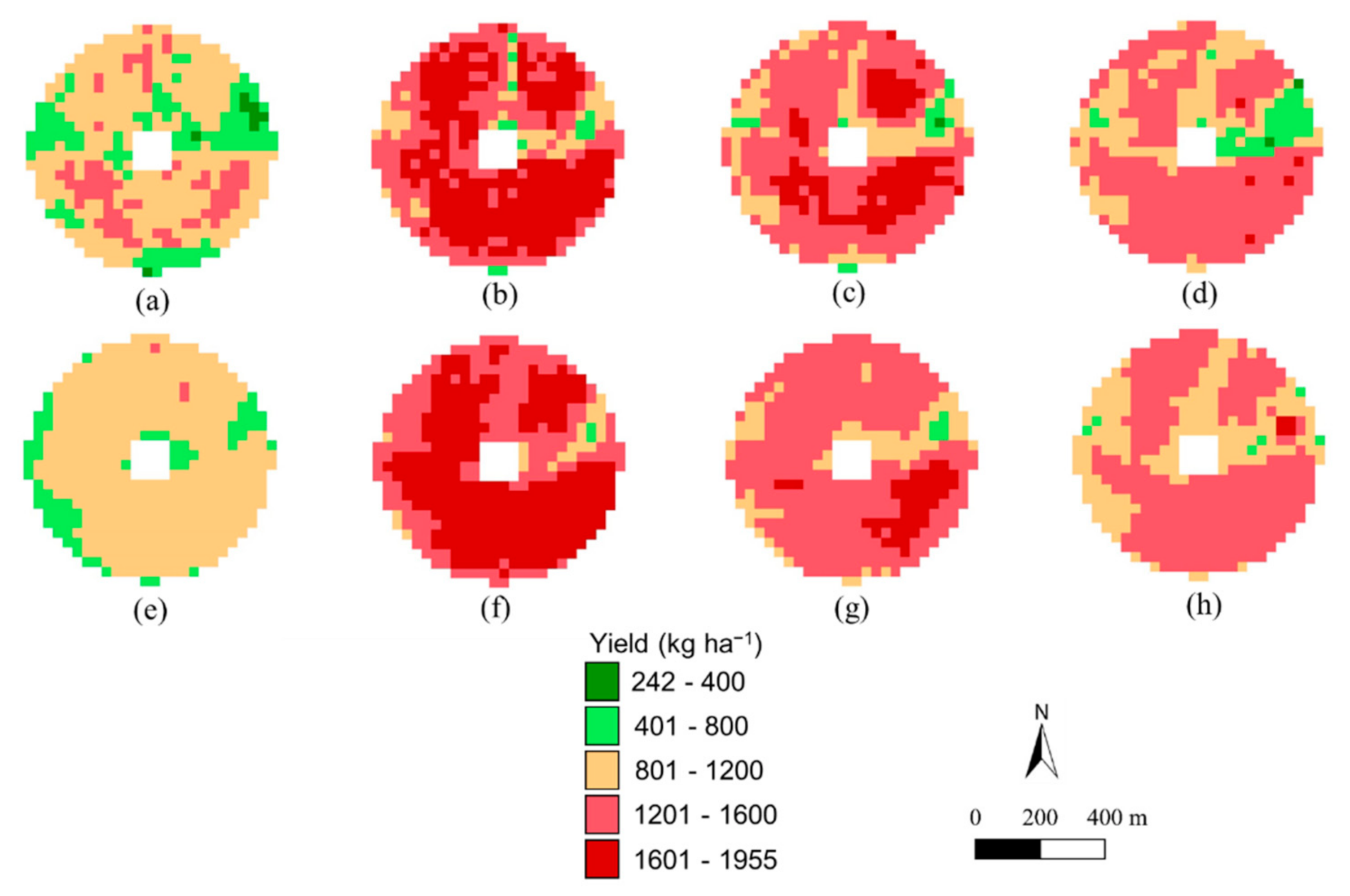
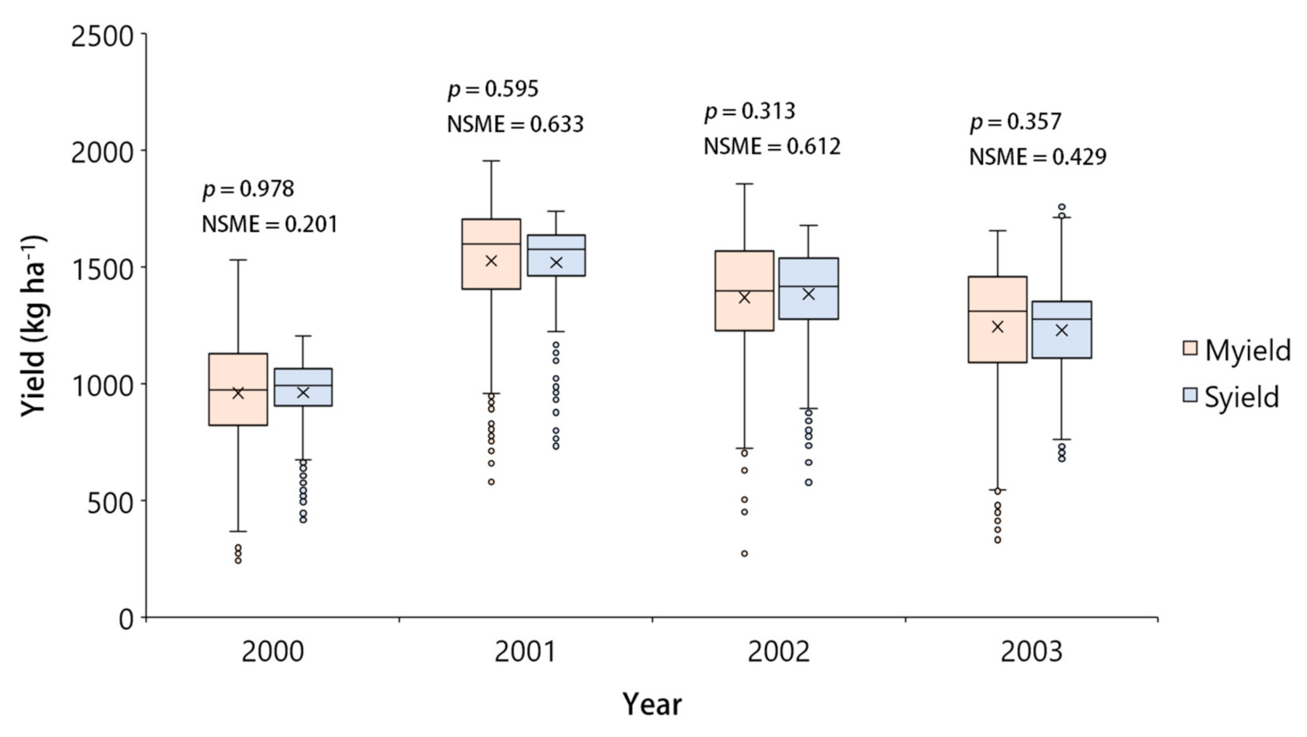
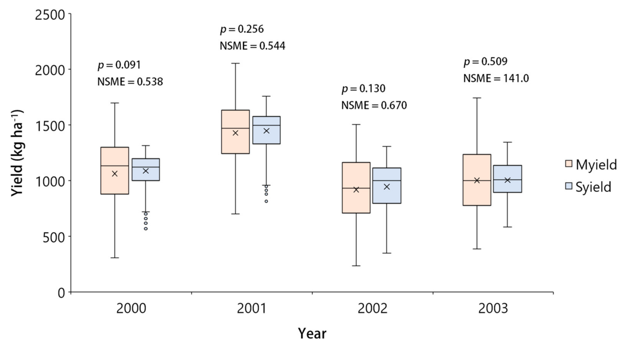
We found that the RSCM cotton system could reproduce spatiotemporal field variations in lint yield at Halfway fields #26 and #28 in the Texas High Plains region (Figure 6 and Figure A2). The simulated lint yields agreed with the measured yields without significant differences at the two locations over four years (Figure 7 and Figure A3). For example, the p-value, NSME value, MAE value, and RMSE value were 0.978, 0.201, 168.6 kg ha⁻¹, and 212.1 kg ha⁻¹, respectively, in 2000; 0.595, 0.633, 117.8 kg ha⁻¹, and 161.2 kg ha⁻¹, respectively, in 2001; 0.313, 0.612, 121.8 kg ha⁻¹, and 164.5 kg ha⁻¹, respectively, in 2002; and 0.357, 0.429, 160.8 kg ha⁻¹, and 200.9 kg ha⁻¹, respectively, in 2003 (Table 2).

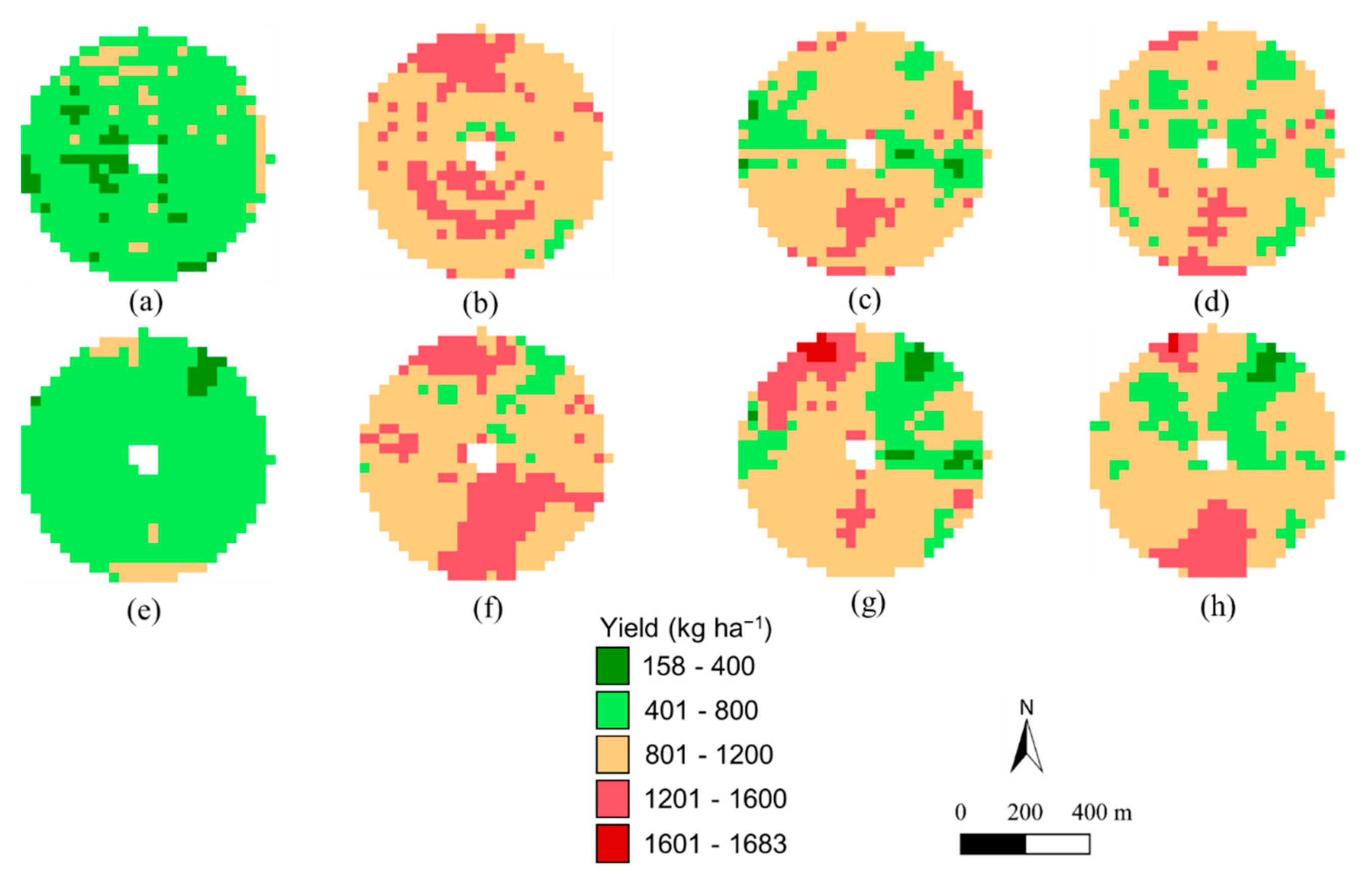
We also demonstrated that the RSCM cotton regime could reproduce lint yields in significant agreement with the measured yields using a separate dataset at field #30 for model validation (Figure 8 and Figure 9). The p-value, NSME value, MAE value, and RMSE value were 0.979, −1.535, 139.5 kg ha⁻¹, and 173.9 kg ha⁻¹, respectively, in 2000; 0.749, 0.053, 141.7 kg ha⁻¹, and 180.3 kg ha⁻¹, respectively, in 2001; 0.823, 0.167, 190.4 kg ha⁻¹, and 243.8 kg ha⁻¹, respectively, in 2002; and 0.848, 0.561, 122.9 kg ha⁻¹, and 155.7 kg ha⁻¹, respectively, in 2003 (Table 2).

Figure 6. Geospatial variations in (a–d) observed and (e–h) simulated cotton lint yield at field #26, Halfway, Texas, USA, in (a,e) 2000, (b,f) 2001, (c,g) 2002, and (d,h) 2003.

Figure 6. Geospatial variations in (a–d) observed and (e–h) simulated cotton lint yield at field #26, Halfway, Texas, USA, in (a,e) 2000, (b,f) 2001, (c,g) 2002, and (d,h) 2003.

Figure 7. Box and whisker plots comparing p values according to the t-test (α = 0.05) and Nash–Sutcliffe model efficiency (NSME) values for the simulated (S) and measured (M) cotton lint yields of field #26 over time. Error bars and boxes represent the 10th, 25th, 75th, and 90th percentiles of the yield data, showing the median (solid line) and mean (×), where circles indicate outliers.

Figure 7. Box and whisker plots comparing p values according to the t-test (α = 0.05) and Nash–Sutcliffe model efficiency (NSME) values for the simulated (S) and measured (M) cotton lint yields of field #26 over time. Error bars and boxes represent the 10th, 25th, 75th, and 90th percentiles of the yield data, showing the median (solid line) and mean (×), where circles indicate outliers.

Figure 8. Geospatial variations in (a–d) observed and (e–h) simulated cotton lint yield at field #30, Halfway, Texas, USA, in (a,e) 2000, (b,f) 2001, (c,g) 2002, and (d,h) 2003.

Figure 8. Geospatial variations in (a–d) observed and (e–h) simulated cotton lint yield at field #30, Halfway, Texas, USA, in (a,e) 2000, (b,f) 2001, (c,g) 2002, and (d,h) 2003.

Figure 9. Box and whisker plots comparing p values according to the t-test (α = 0.05) and Nash–Sutcliffe model efficiency (NSME) values for the simulated (S) and measured (M) cotton lint yields of field #30 over time. Error bars and boxes represent the 10th, 25th, 75th, and 90th percentiles of the yield data, showing the median (solid line) and mean (×), where circles indicate outliers.

Figure 9. Box and whisker plots comparing p values according to the t-test (α = 0.05) and Nash–Sutcliffe model efficiency (NSME) values for the simulated (S) and measured (M) cotton lint yields of field #30 over time. Error bars and boxes represent the 10th, 25th, 75th, and 90th percentiles of the yield data, showing the median (solid line) and mean (×), where circles indicate outliers.

Table 2. Comparison statistics of p (t-test at α = 0.05), mean absolute error (MAE), root mean square deviation (RMSD) and Nash–Sutcliffe model efficiency (NSME) for the simulated and observed cotton yields of the fields #26, #28, and #30.

Field #	Year	Mean (Median) ± 1 SD		p	MAE	RMSD	NSME
		Simulated	Observed
		kg ha−1		Unitless	kg ha−1		Unitless
26	2000	961.5 (994.1) ± 146.3	961.2 (975.1) ± 237.4	0.978	168.6	212.1	0.201
	2001	1518.9 (1576.2) ± 178.0	1526.7 (1597.7) ± 266.4	0.595	117.8	161.2	0.633
	2002	1384.8 (1417.1) ± 196.9	1369.6 (1397.3) ± 264.3	0.313	121.8	164.5	0.612
	2003	1230.0 (1277.0) ± 183.9	1243.8 (1312.6) ± 270.3	0.357	132.1	204.2	0.429
28	2000	1088.1 (1122.8) ± 160.8	1063.2 (1131.8) ± 296.0	0.091	160.8	200.9	0.538
	2001	1446.8 (1496.3) ± 184.8	1428.9 (1471.8) ± 297.9	0.256	157.7	201.1	0.544
	2002	945.3 (1001.6) ± 233.9	919.7 (933.4) ± 295.9	0.130	134.8	169.8	0.670
	2003	1038.6 (1045.8) ± 190.3	1049.4 (1053.4)± 311.2	0.509	141.0	172.1	0.694
30	2000	604.4 (613.9) ± 143.4	604.6 (595.7) ± 109.3	0.979	139.5	173.9	−1.535
	2001	1104.5 (1101.6) ± 146.0	1107.9 (1121.9) ± 185.4	0.749	141.7	180.3	0.053
	2002	949.7 (980.3) ± 208.9	953.1 (974.3) ± 267.3	0.823	190.4	243.8	0.167
	2003	952.7 (941.9) ± 167.4	950.2 (944.8) ± 235.0	0.848	122.9	155.7	0.561

Table 2. Comparison statistics of p (t-test at α = 0.05), mean absolute error (MAE), root mean square deviation (RMSD) and Nash–Sutcliffe model efficiency (NSME) for the simulated and observed cotton yields of the fields #26, #28, and #30.

Field #	Year	Mean (Median) ± 1 SD		p	MAE	RMSD	NSME
		Simulated	Observed
		kg ha−1		Unitless	kg ha−1		Unitless
26	2000	961.5 (994.1) ± 146.3	961.2 (975.1) ± 237.4	0.978	168.6	212.1	0.201
	2001	1518.9 (1576.2) ± 178.0	1526.7 (1597.7) ± 266.4	0.595	117.8	161.2	0.633
	2002	1384.8 (1417.1) ± 196.9	1369.6 (1397.3) ± 264.3	0.313	121.8	164.5	0.612
	2003	1230.0 (1277.0) ± 183.9	1243.8 (1312.6) ± 270.3	0.357	132.1	204.2	0.429
28	2000	1088.1 (1122.8) ± 160.8	1063.2 (1131.8) ± 296.0	0.091	160.8	200.9	0.538
	2001	1446.8 (1496.3) ± 184.8	1428.9 (1471.8) ± 297.9	0.256	157.7	201.1	0.544
	2002	945.3 (1001.6) ± 233.9	919.7 (933.4) ± 295.9	0.130	134.8	169.8	0.670
	2003	1038.6 (1045.8) ± 190.3	1049.4 (1053.4)± 311.2	0.509	141.0	172.1	0.694
30	2000	604.4 (613.9) ± 143.4	604.6 (595.7) ± 109.3	0.979	139.5	173.9	−1.535
	2001	1104.5 (1101.6) ± 146.0	1107.9 (1121.9) ± 185.4	0.749	141.7	180.3	0.053
	2002	949.7 (980.3) ± 208.9	953.1 (974.3) ± 267.3	0.823	190.4	243.8	0.167
	2003	952.7 (941.9) ± 167.4	950.2 (944.8) ± 235.0	0.848	122.9	155.7	0.561

4. Discussion

This study evaluated and tested a crop modeling system that integrated proximal and remote sensing information to simulate the spatiotemporal variations in cotton growth and lint yield. The current simulation study using the updated RSCM cotton system demonstrated that it is possible to simulate temporal variations in cotton growth and lint yield in fields at different locations and with various irrigation systems. Furthermore, the simulation results using the Landsat satellite imagery showed that RSCM cotton could reproduce spatiotemporal variations in lint yield induced by different field conditions and climate variability. In addition, our findings verified the ability of RSCM cotton to use LAI data to minimize the inaccuracies between the simulated and observed canopy growth variables.

The ability to perform mid-season calibration allowed RSCM cotton to reproduce cotton growth and lint yields using proximally or remotely sensed data. This process also required minimal environmental data input [10,23]. Furthermore, the method has been validated for use for several staple crops using inputs from various proximal or remote sensing platforms from a range of fields [18,19,20]. Thus, the modeling system could facilitate the monitoring of growth conditions for multiple crops and may be able to accurately predict yield. However, limitations exist because of the model’s strong dependency on proximal or remote sensing data. Hereafter, we discuss the reliance of RSCM cotton on the timing, spatial resolution, and area coverage information provided by the remotely sensed data.

We estimated LAI from VI using an empirical modeling approach reliant on inputs from remotely sensed data. We assumed that the LAI and NDVI relationships at the proposed cotton fields were consistent with the experimental data obtained at PSWCL over three years (2003–2005). VI has been frequently used as an indicator of the canopy conditions of crops and has delivered the information required to accurately determine crop growth and yield [4,33,34]. However, VI data collected too early or too late during the growing season may yield poor estimates of the actual canopy conditions. Furthermore, similar to the RSCM system, VI data are not accurate when only single data points are provided as input [35]. However, agreement between the simulation and field measurements could be achieved when several evenly distributed data points representative of crop conditions over the growing season were provided. Therefore, the timing of remote sensing data acquisition is crucial for increasing simulation accuracy.

Crop models are usually created to simulate crop responses to changes in the surrounding environment, thus helping to establish practices for ideal growth and optimum crop management [36]. Previously, efforts have been made to establish parameter estimate protocols for crop modeling to simplify the models and to minimize differences between simulations and measurements [23,37]. A properly calibrated crop model can precisely reproduce crop growth and productivity, as well as environmental factors such as soil water content [37]. The RSCM system can easily perform these functions, and is designed to simulate crop growth and productivity with simple input prerequisites that integrate proximal or remote sensing data. There have been many attempts to establish similar integrated crop modeling systems for various staple crops, including rice [10] and wheat [18]. The proposed RSCM cotton system could simulate cotton growth and productivity with statistically significant precision. We showed that RSCM cotton produced simulated LAI and lint yield values that were in statistically significant agreement with the corresponding measured values across multiple locations and irrigation treatment conditions. Therefore, the integrated cotton-modeling system has potential for application in simulation case studies of other cultivation and management systems. This system could be applied to determine appropriate planting and N treatments and to model geospatial variations in growth and productivity by employing pixel-based, two-dimensional simulations. The results of the current study also suggest that the RSCM system could be applied to cotton growth and lint yield monitoring using operational satellite information.

Crop monitoring tasks using satellite remote sensing involve two conflicting criteria for data acquisition: a high pixel resolution and large coverage area. Although the RSCM cotton system can be applied to cotton growth simulation over large areas, it has limited simulation performance because of its inaccurate representation of plant canopy conditions. This inaccuracy was mainly attributable to the low ground resolution of satellite images with mixed pixels. The orbital height, swath width, and revisit time of a satellite system affect the spatial resolution of satellite imagery [2,38]. It is also challenging to acquire satellite images over large areas within a short period of time using satellite platforms aboard very high-ground resolution sensors, e.g., GeoEye-2 (https://www.aerospace-technology.com/projects/geoeye-2-satellite/, accessed on 1 February 2022) and WorldView-3 (https://earth.esa.int/eogateway/missions/worldview-3, accessed on 1 February 2022). These satellite systems are generally designed for observing relatively narrow swaths. Other satellite sensors with a coarse ground resolution, e.g., MODIS (https://modis.gsfc.nasa.gov/, accessed on 1 February 2022), benefit from higher revisit rates and more comprehensive area coverage. However, these satellite sensors do not capture the detailed spectral characteristics of homogeneous crop conditions as they have low ground resolution [39]. Therefore, identifying the optimum ground resolution for applying satellite data to the RSCM cotton system is necessary for practical modeling applications. The data regarding spectral crop characteristics from satellite images can be determined with homogeneous types from mixed pixels using simple data processing strategies. Following this, the RSCM cotton system could be used to produce an effective crop information delivery system that utilizes satellite imagery data with a rapid data processing pipeline. In this context, Landsat imagery, which has a pixel resolution of 30 m and a swath width of 185 km, would be ideal for monitoring and mapping agricultural lands and crop productivities in medium-sized farms [40,41], in comparison with the other medium resolution satellite images including those from MODIS. The mission of Landsat was to help land managers, researchers, and policymakers make informed decisions about natural and agricultural resources and the environment.

We observed that the simulated lint yields often had fewer field variabilities than the corresponding measured values in this study. One of the reasons for this disagreement was the lack of sensitivity of the wavebands regarding the spectral resolution used in the satellite images collected for the crop canopy. The RSCM system, which employs remote sensing imagery, requires accurately quantified image data to generate specific growth information on the crop of interest during its growing season [10,35]. Once this issue is resolved, the application of RSCM is likely to increase. A relatively sophisticated and dependable satellite sensor should be used to complement radiometrically well-calibrated imagery. Increasing the resolution of remote sensing images can help increase the applicability of this system for monitoring crop growth conditions and productivity [40]. Determining the optimum wavelength ranges for the highest spectral resolution was out of the scope of the current study, but would be a worthwhile direction for a future study.

The RSCM system can be further developed into an information delivery system to inform decisions regarding crop management and cultivation, thus ultimately increasing crop productivity. We believe that this improved system would increase the precision of many agricultural management practices. Future enhancements that could be made to improve the modeling system include enhancing the forecast capability, both short-term (within the crop growing season) and long-term. These enhancements would also mean that the RSCM could be used as a decision support system to improve various management practices in response to changing environments.

5. Conclusions

The current study demonstrated that the updated RSCM cotton technology could reproduce spatiotemporal variations in cotton productivity across multiple locations and irrigation systems. RSCM cotton simulated cotton canopy growth and lint yield, producing data that agreed with corresponding field measurements without significant differences. This study introduced the RSCM cotton system for reproducing field-based geospatial variations in cotton lint yield. We believe that this modeling system is applicable for scouting cotton growth, evaluating productivity, and acting as a field management support tool, owing to the integration of proximal and remote sensing information. An advantage of the RSCM cotton system is that users can operate it with minimal climate data regarding solar radiation, temperatures, and proximal or remote sensing information. This is possible because of the integration of proximal or remote sensing information into the crop modeling technology, an advancement that reduces input requirements. The proposed RSCM for cotton requires accurately quantified proximal or remote sensing data or imagery to improve its ability to monitor crop productivity and, ultimately, to inform field management decisions.

References

1. Martin, J.D.; Leonard, W.H.; Stamp, D.L.; Waldren, R.P. Principles of Field Crop Production, 4th ed.; Pearson: New York, NY, USA, 2005. [Google Scholar]
2. Campbell, J.B.; Wynne, R.H. Introduction to Remote Sensing; Guilford Press: New York, NY, USA, 2011. [Google Scholar]
3. Dorigo, W.A.; Zurita-Milla, R.; De Wit, A.J.W.; Brazile, J.; Singh, R.; Schaepman, M.E. A review on reflective remote sensing and data assimilation techniques for enhanced agroecosystem modeling. Int. J. Appl. Earth Obs. Geoinf. 2007, 9, 165–193. [Google Scholar] [CrossRef]
4. Zarco-Tejada, P.J.; Ustin, S.L.; Whiting, M.L. Temporal and spatial relationships between within-field yield variability in cotton and high-spatial hyperspectral remote sensing imagery. Agron. J. 2005, 97, 641–653. [Google Scholar] [CrossRef] [Green Version]
5. Kern, A.; Barcza, Z.; Marjanović, H.; Árendás, T.; Fodor, N.; Bónis, P.; Bognár, P.; Lichtenberger, J. Statistical modelling of crop yield in Central Europe using climate data and remote sensing vegetation indices. Agric. For. Meteorol. 2018, 260–261, 300–320. [Google Scholar] [CrossRef]
6. Labus, M.P.; Nielsen, G.A.; Lawrence, R.L.; Engel, R.; Long, D.S. Wheat yield estimates using multi-temporal NDVI satellite imagery. Int. J. Remote Sens. 2002, 23, 4169–4180. [Google Scholar] [CrossRef]
7. Delécolle, R.; Maas, S.; Guérif, M.; Baret, F. Remote sensing and crop production models: Present trends. ISPRS J. Photogramm. Remote Sens. 1992, 47, 145–161. [Google Scholar] [CrossRef]
8. Becker-Reshef, I.; Vermote, E.; Lindeman, M.; Justice, C. A generalized regression-based model for forecasting winter wheat yields in Kansas and Ukraine using MODIS data. Remote Sens. Environ. 2010, 114, 1312–1323. [Google Scholar] [CrossRef]
9. Moulin, S.; Bondeau, A.; Delecolle, R. Combining agricultural crop models and satellite observations: From field to regional scales. Int. J. Remote Sens. 1998, 19, 1021–1036. [Google Scholar] [CrossRef]
10. Nguyen, V.C.; Jeong, S.; Ko, J.; Ng, C.T.; Yeom, J. Mathematical integration of remotely-sensed information into a crop modelling process for mapping crop productivity. Remote Sens. 2019, 11, 2131. [Google Scholar] [CrossRef] [Green Version]
11. Jones, J.W.; Hoogenboom, G.; Porter, C.H.; Boote, K.J.; Batchelor, W.D.; Hunt, L.A.; Wilkens, P.W.; Singh, U.; Gijsman, A.J.; Ritchie, J.T. The DSSAT cropping system model. Eur. J. Agron. 2003, 18, 235–265. [Google Scholar] [CrossRef]
12. Hijmans, R.J.; Guiking-Lens, I.; Van Diepen, C. WOFOST 6.0: User’s Guide for the WOFOST 6.0 Crop Growth Simulation Model; D.L.O. Winand Staring Centre: Wageningen, The Netherlands, 1994; p. 145. [Google Scholar]
13. Zhang, X.; Zhang, Q. Monitoring interannual variation in global crop yield using long-term AVHRR and MODIS observations. ISPRS J. Photogramm. Remote Sens. 2016, 114, 191–205. [Google Scholar] [CrossRef]
14. Khanal, S.; Kc, K.; Fulton, J.; Shearer, S.; Ozkan, E. Remote Sensing in Agriculture—Accomplishments, Limitations, and Opportunities. Remote Sens. 2020, 12, 3783. [Google Scholar] [CrossRef]
15. Huang, J.; Gómez-Dans, J.; Huang, H.L.; Ma, H.; Wu, Q.; Lewis, P.E.; Liang, S.; Chen, Z.; Xue, J.; Wu, Y.; et al. Assimilation of remote sensing into crop growth models: Current status and perspectives. Agric. For. Meteorol. 2019, 276–277, 107609. [Google Scholar] [CrossRef]
16. Huang, Y.; Ryu, Y.; Jiang, C.; Kimm, H.; Kim, S.; Kang, M.; Shim, K. BESS-Rice: A remote sensing derived and biophysical process-based rice productivity simulation model. Agric. For. Meteorol. 2018, 256–257, 253–269. [Google Scholar] [CrossRef]
17. Jin, X.; Kumar, L.; Li, Z.; Feng, H.; Xu, X.; Yang, G.; Wang, J. A review of data assimilation of remote sensing and crop models. Eur. J. Agron. 2018, 92, 141–152. [Google Scholar] [CrossRef]
18. Shin, T.; Ko, J.; Jeong, S.; Shawon, A.R.; Lee, K.D.; Shim, S.I. Simulation of wheat productivity using a model integrated with proximal and remotely controlled aerial sensing information. Front. Plant Sci. 2021, 12, 649660. [Google Scholar] [CrossRef]
19. Shawon, A.R.; Ko, J.; Ha, B.; Jeong, S.; Kim, D.K.; Kim, H.-Y. Assessment of a proximal sensing-integrated crop model for simulation of soybean growth and yield. Remote Sens. 2020, 12, 410. [Google Scholar] [CrossRef] [Green Version]
20. Yeom, J.-M.; Jeong, S.; Jeong, G.; Ng, C.T.; Deo, R.C.; Ko, J. Monitoring paddy productivity in North Korea employing geostationary satellite images integrated with GRAMI-rice model. Sci. Rep. 2018, 8, 16121. [Google Scholar] [CrossRef] [Green Version]
21. Ko, J.; Maas, S.J.; Lascano, R.J.; Wanjura, D. Modification of the GRAMI Model for Cotton. Agron. J. 2005, 97, 1374–1379. [Google Scholar] [CrossRef] [Green Version]
22. Maas, S.J. Parameterized model of gramineous crop growth: I. leaf area and dry mass simulation. Agron. J. 1993, 85, 348–353. [Google Scholar] [CrossRef]
23. Maas, S.J. Parameterized model of gramineous crop growth: II. within-season simulation calibration. Agron. J. 1993, 85, 354–358. [Google Scholar] [CrossRef]
24. Ko, J.; Maas, S.J.; Mauget, S.; Piccinni, G.; Wanjura, D. Modeling water-stressed cotton growth using within-season remote sensing data. Agron. J. 2006, 98, 1600–1609. [Google Scholar] [CrossRef] [Green Version]
25. Guo, W.; Maas, S.; Lascano, R.; Brightbill, J. Mapping spatial and temporal variability of cotton yield in West Texas. In Proceedings of the Beltwide Cotton Conferences, New Orleans, LA, USA, 4–7 January 2005; pp. 2067–2073. [Google Scholar]
26. Guo, W. Spatial and Temporal Variability in Cotton Yield in Relation to Soil Apparent Electrical Conductivity, Topography, and Remote Sensing Imagery; Texas Tech University: Lubbock, TX, USA, 2005. [Google Scholar]
27. Rajapakse, S. Automated Radiometric Normalization Technique for Multitemporal Landsat-TM and ETM+ Imagery; Texas Tech University: Lubbock, TX, USA, 2005. [Google Scholar]
28. Monteith, J.L. Solar radiation and productivity in tropical ecosystems. J. Appl. Ecol. 1972, 9, 747–766. [Google Scholar] [CrossRef] [Green Version]
29. Monteith, J.; Unsworth, M. Principles of Environmental Physics: Plants, Animals, and the Atmosphere, 4th ed.; Academic Press: San Diego, CA, USA, 2013. [Google Scholar]
30. Press, W.H.; Teukolsky, S.A.; Vetterling, W.T.; Flannery, B.P. Numerical Recipes: The Art of Scientific Computing; Cambridge University Press: New York, NY, USA, 1992. [Google Scholar]
31. Nash, J.C. Compact Numerical Methods for Computers: Linear Algebra and Function Minimisation; CRC Press: New York, NY, USA, 1990. [Google Scholar]
32. Nash, J.E.; Sutcliffe, J.V. River flow forecasting through conceptual models part I—A discussion of principles. J. Hydrol. 1970, 10, 282–290. [Google Scholar] [CrossRef]
33. Johnson, D.M. An assessment of pre- and within-season remotely sensed variables for forecasting corn and soybean yields in the United States. Remote Sens. Environ. 2014, 141, 116–128. [Google Scholar] [CrossRef]
34. Bolton, D.K.; Friedl, M.A. Forecasting crop yield using remotely sensed vegetation indices and crop phenology metrics. Agric. For. Meteorol. 2013, 173, 74–84. [Google Scholar] [CrossRef]
35. Ko, J.; Jeong, S.; Yeom, J.; Kim, H.; Ban, J.-O.; Kim, H.-Y. Simulation and mapping of rice growth and yield based on remote sensing. J. Appl. Remote Sens. 2015, 9, 096067. [Google Scholar] [CrossRef]
36. Lövenstein, H.; Rabbinge, R.; van Keulen, H. World Food Production, Textbook 2: Biophysical Factors in Agricultural Production; Wageningen University & Research: Wageningen, The Netherlands, 1992. [Google Scholar]
37. Ahuja, L.R.; Rojas, K.W.; Hanson, J.D.; Shaffer, M.J.; Ma, L. Root Zone Water Quality Model: Modeling Management Effects on Water Quality and Crop Production; Water Resources Publications, LLC: Highland Ranch, CO, USA, 2000. [Google Scholar]
38. Verburg, P.H.; Neumann, K.; Nol, L. Challenges in using land use and land cover data for global change studies. Glob. Change Biol. 2011, 17, 974–989. [Google Scholar] [CrossRef] [Green Version]
39. Ozdogan, M.; Woodcock, C.E. Resolution dependent errors in remote sensing of cultivated areas. Remote Sens. Environ. 2006, 103, 203–217. [Google Scholar] [CrossRef]
40. Som-Ard, J.; Atzberger, C.; Izquierdo-Verdiguier, E.; Vuolo, F.; Immitzer, M. Remote sensing applications in sugarcane cultivation: A review. Remote Sens. 2021, 13, 4040. [Google Scholar] [CrossRef]
41. Dong, J.; Xiao, X.; Menarguez, M.A.; Zhang, G.; Qin, Y.; Thau, D.; Biradar, C.; Moore, B., III. Mapping paddy rice planting area in northeastern Asia with Landsat 8 images, phenology-based algorithm and Google Earth Engine. Remote Sens. Environ. 2016, 185, 142–154. [Google Scholar] [CrossRef] [Green Version]
Figure 2. Diagrammatic representation of the remote sensing-integrated crop model (RSCM) for cotton: (a) cotton growth simulation (CGS) procedure and (b) optimization of model parameters using proximal or remote sensing information. AGDM, LAI, PAR, and RS represent above-ground dry mass, leaf area index, photosynthetically active radiation, and remote sensing, respectively.
Remotesensing 14 01421 g002
Figure 3. Relationship between leaf area index (LAI) and normalized difference vegetation index (NDVI) using the dataset obtained from the plant stress and water conservation laboratory in Lubbock, Texas, USA, from 2003 to 2005.
Remotesensing 14 01421 g003
Figure 4. Simulated and observed cotton growth from Texas, USA at (a) field #26 in Halfway, HW in 2002; (b) the Texas A&M University Agricultural Research field in Lamesa, LMS in 1999; and (c) the Plant Stress and Water Conservation Laboratory field in Lubbock, LBK in 2002. (d) Comparison between simulated and observed lint yields for all data from the study sites. OLAI, SLAI, and SAGDM represent observed leaf area index, simulated leaf area index, and simulated above-ground dry mass, respectively. #26, #28, and #33 represent cotton field circles.
Remotesensing 14 01421 g004
Figure 5. Simulated and observed cotton growth at irrigation intervals of (a) 5.5 h and (b) 6.5 h in 2003, and (c) with 2 mm irrigation in 2005 at the Plant Stress and Water Conservation Laboratory field in Lubbock, Texas, USA (d) Comparison between simulated and observed lint yields for all irrigation treatments. OLAI, SLAI, and SAGDM represent observed leaf area index, simulated leaf area index, and simulated above-ground dry mass, respectively.
Remotesensing 14 01421 g005