Abstract
Affected by the spatial environment, the accuracy and stability of ultra-wideband (UWB) positioning in a narrow space are significantly lower than those in the general indoor environment, which limits navigation and positioning services in a complex scene. To improve the positioning accuracy and stability of a narrow space, this study proposed a positioning algorithm by combining Kalman filter (KF) and dilution of precision (DOP). Firstly, we calculated the DOP values of the target narrow space by changing the location of the test nodes throughout the space. Secondly, the initial coordinate values of the test nodes were calculated by the weighted least squares (WLS) positioning algorithm and were used as the observation values of KF. Finally, the DOP values were adaptively introduced into KF to update the coordinates of the nodes to be tested. The proposed algorithm was tested in two narrow scenes with different length–width ratios. The experimental results showed that the DOP values of the narrow space were much higher than that of the wide space. Furthermore, even if the ranging error was low, the positioning error was high in the narrow space. The proposed fusion positioning algorithm reported a higher positioning accuracy in the narrow space, and the higher DOP values of the scene, the greater the accuracy improvement of the algorithm. This study reveals that no matter how the base stations are configured, the DOP values of the narrow space are much higher than that of the wide space, thus causing larger positioning errors. The proposed positioning algorithm can effectively suppress the positioning error caused by the narrow spatial structure, so as to improve the positioning accuracy and stability.
1. Introduction
In recent years, with the development of the Internet of Things (IoT), virtual reality and smart home technology, the demand for indoor location services has increased [1,2]. Low-cost, high-precision indoor positioning solutions have become the key to many IoT applications [3,4,5]. The ranging technology of ultra-wideband (UWB) has the advantages of a short pulse interval and high temporal resolution, which can achieve centimeter-level ranging accuracy [1,6]. Therefore, UWB has become a common technology for indoor positioning in recent years [7].
Furthermore, a series of studies have been carried out on the UWB positioning mechanism, including channel model [8], multipath component estimation [9] and non-line-of-sight (NLOS) identification [10]. However, most studies have not focused on a special scene such as a narrow space. Most application scenes contain the narrow space, such as coal mine roadway, shaft, tunnel, corridor, etc. [11], whose structural characteristics can be summarized as follows: the space is long and narrow, and the side wall is limited [12]. Owing to these special structure characteristics, the positioning is more challenging in the narrow space compared with the general indoor environment. Firstly, in the narrow space, the electromagnetic wave propagation will have various reflections, transmissions, refractions and keyhole effects, resulting in channel deterioration and ranging errors [13,14]. Secondly, the narrow space limits the layout of the positioning base station, which means the base station layout is impossible to be ideal for positioning [15]. Therefore, it is difficult to obtain a high positioning accuracy for UWB positioning in a narrow indoor space. Improving the positioning accuracy in the narrow space will push the UWB positioning to a wider range of application scenes [16].
DOP is an important indicator to describe the position accuracy obtained from a satellite constellation [17,18], which is closely related to the satellite network structure. In the indoor environment, it contains the knowledge of positioning accuracy under specific base station network and scene characteristics [19]. In recent years, DOP has also become an important indicator of the geometric location distribution and accuracy of base stations in indoor positioning. The applicability of DOP in an indoor time difference of an arrival (TDOA) positioning system is analyzed in [20]. The results showed that, in the case of a low signal-to-noise ratio, the DOP values can be used as a reference index for the optimization of base station configuration. In [21], the base station layout schemes in different scenes were simulated to minimize the positioning error and maximize the coverage of the positioning area. Similarly, in [22], the optimal positioning scheme was obtained by weighting the geometric dilution of precision (GDOP) values, thereby minimizing the influence of the NLOS error in the position estimation process. Most of the previous studies only analyzed the characteristics of the geometric structure between the positioning source and the positioning node by employing DOP values, which gave the corresponding base station layout optimization strategy. However, they did not, in turn, use the DOP numerical analysis model to improve the positioning accuracy and stability of the existing positioning algorithm in a narrow space.
The Kalman filter (KF) algorithm is an optimal regression data processing algorithm [23,24]. It has been widely used to estimate the optimal state in various fields of engineering, such as robotics, target tracking, navigation, signal processing and communication [25,26,27]. In the study of indoor positioning, the estimation position of the tag is mainly optimized by KF. In [28], the particle swarm optimization algorithm was used to optimize the parameters of KF to improve the ranging accuracy of UWB. However, this technique was only applicable to one-dimensional ranging. In order to improve the estimation accuracy of nonlinear systems, various improved algorithms have been designed based on KF, such as the extended Kalman filter (EKF) algorithm [29] and the unscented Kalman filter (UKF) algorithm [30]. In [31], a UWB positioning algorithm for an underground coal mine was proposed, which improved the positioning accuracy of the system by introducing the EKF algorithm. Similarly, in [32], an integrated indoor positioning system was proposed by combining IMU and UWB, in which EKF and UKF were employed to improve the positioning accuracy and expand the positioning application scene. Although UKF can effectively reduce the linearization error, the technology is extremely dependent on the initial parameter setting. The initial value setting of the parameters is adjusted manually using a trial-and-error method according to the application. However, this manual method takes more time, and sometimes the filter may diverge [33].
The accuracy of the estimated parameters of the KF technique depends, to a large extent, on the correct knowledge of the covariance matrix Q of its model noise and the covariance matrix R of the measurement noise [34,35]. The statistics of Q and R highly influence the Kalman gain K and, consequently, the error of the measurements, where the covariance matrix R of the measurement noise represents the confidence in the filtering system on the observed values [36]. Meanwhile, the DOP values reflect the sensitivity of the positioning system to the ranging error: the larger the DOP value, the lower the positioning accuracy of the UWB system, and the less credible the positioning output [37]. Therefore, the adaptive combination of the DOP numerical analysis model with the covariance matrix R of the measurement noise of KF can be considered to improve the positioning accuracy of the existing algorithms in the narrow space.
Based on the existing research, this study designed a positioning algorithm that combines the DOP values and KF to improve the positioning accuracy of the narrow space. Firstly, the distribution characteristics of the UWB positioning error in a narrow space are systematically explored using a DOP numerical analysis model. Secondly, based on the initial positioning results acquired by the weighted least square (WLS) positioning algorithm, the DOP numerical analysis model was adaptively combined with KF to solve the problem of positioning misalignment in a narrow space. Finally, the proposed algorithm was tested on two narrow scenes with different length–width ratios. Both static and dynamic positioning results were reported in the experiments.
2. Methods
The positioning framework is shown in Figure 1. Firstly, the distance between the UWB base stations and the tag was measured by double-sided two-way ranging to complete the initial data acquisition. Based on the ranging data, the WLS method was used to calculate the initial coordinate of the tag, which was considered as the observation values of KF. Secondly, the position dilution of precision (PDOP) value of the positioning scene was acquired by the DOP numerical analysis model, and it was used as the reference value of the observation noise covariance of KF. Finally, the state equation of the system was constructed by Taylor expansion to complete the positioning algorithm.
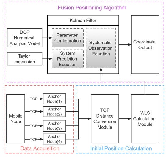
Figure 1.
Framework of the positioning algorithm.
2.1. Positioning Algorithm and DOP Numerical Distribution Model
Suppose that there are m positioning base stations in the two-dimensional space and their coordinates are . There are certain tags (the positions are unknown) to be tested in the space, and their coordinates are . Through TOA measurement, the measurement distance from the tag to the ith base station can be obtained. Therefore, the TOA measurement model can be expressed as follows [38]:
where represents the distance between the ith base station and the tag; represents the ranging error of TOA. When calculating the coordinates of the tag, the coordinates of the positioning base station and the measurement distance are known. Therefore, the tag position can be solved by the following mathematical model:
Equation (2) can be transformed into the matrix form: AX = B, which can be solved using the least square (LS) method [39]:
In general, the coordinate information of the tag is calculated by the LS method. However, the LS method is based on the assumption that the ranging error has a constant variance. In the actual measurement, the ranging error is changing [40]. At this time, the WLS method can be used to solve the above problems. This method mainly introduces a weighted matrix to multiply the ranging error of a single range by the estimated range to obtain more reliable results. The positive definite weighted matrix W with diagonal m is as follows:
In Equation (4), the element in the positive definite weighted matrix W can be calculated by measuring the reciprocal of the product of distance and ranging error [41]. At this point, the estimated position of the tag can be expressed in the WLS estimator:
Its covariance matrix can be expressed as:
In general, the horizontal dilution of precision (HDOP) and PDOP can be derived from the covariance matrix computed from the error equation [42]:
From the above equations, it is not difficult to find that the HDOP and PDOP values are obtained by the LS estimation, and their values reflect the possible accuracy of UWB measurement positioning. The size of the PDOP values is positively correlated with the error of the base station positioning. The larger the PDOP values, the greater the amplification of the ranging error by the positioning algorithm, and the lower the positioning accuracy of the system [18]. In order to improve the positioning accuracy when the PDOP values are far greater than the normal value, the positioning error can be reduced by combining the PDOP numerical analysis model with KF. In this study, we calculated the PDOP values by changing the location of the test node throughout the space.
2.2. Optimized Kalman Filter Parameter Configuration Based on DOP Values
The KF algorithm mainly consists of a prediction step and an update step. The closer the state estimation equation is to the actual process, the higher the prior estimation accuracy is [43]. The accuracy of the posteriori estimation results mainly depends on the observed values. The smaller the error of the observed data obtained by the sensor, the higher the accuracy of the optimal estimation of the KF algorithm [44]. The specific process of the algorithm is detailed below [24].
The linear system’s state and observation equations are as follows:
where is the state vector, F is the linear system transfer matrix, is the process noise vector, is the observation vector, H is the state variable to observation transition matrix, and is the process noise vector. The true state of the system can be predicted from the state of the system at the previous moment and the observed state at the next moment. The specific solution equation is as follows:
- (1)
- Prediction steps:
- (2)
- Supplementary Kalman gain:
- (3)
- Update steps:
In Equations (11) to (13), and are the prior estimated state vector and posterior estimated state vector at epoch . and are covariance matrix of prior estimation and the covariance matrix of posteriori estimation at epoch . is the linear system transfer matrix, is the process noise vector, is the Kalman gain, is the state transition matrix, and R is the measurement errors covariance matrix. is the observation vector.
The source of measurement noise covariance is the observation error [45]. In this study, the source of observation error is mainly from two aspects: the ranging error and tag position solution error. Among them, the ranging error mainly comes from the multipath effect and the NLOS error in the narrow space, and the tag position calculation error mainly comes from the WLS algorithm.
According to Equation (6), Q is the covariance matrix of the estimated position of the label. It can therefore be used as a reference value for the measurement noise covariance. Since another part of the observation error comes from multipath effects and NLOS errors in a narrow space, an environmental factor K can be set as an adjustment. Thus, the measurement noise covariance can be expressed as follows:
2.3. Fusion Positioning Algorithm
In this study, a fusion positioning algorithm was designed by combining the DOP numerical analysis model, WLS algorithm and KF algorithm. The system state equation was constructed using Taylor expansion. The coordinate solution of the WLS positioning algorithm was used as the observation value of KF. DOP was introduced into the measurement noise covariance parameter of the KF observation equation to suppress the positioning error in the narrow space. The specific algorithm procedure is as follows:
- Building the system model:
The prediction equation and observation equation of the system are constructed according to Equations (9) and (10). Considering that the position of the moving object will not change exponentially, the second-order Taylor expansion of at can be carried out to complete the construction of the prediction equation. In this way, the transfer matrix F in Equation (9) can be acquired. In addition, since this study regards the output coordinates of WLS as the observed values, which is close to the position state value, we replace the observation transition matrix H in Equation (10) with the unit matrix I in the experiment. Consequently, Equations (15) and (16) are, respectively, the prediction equation and observation equation:
- 2.
- Measuring system observation value X:
Based on the transceiver information between UWB devices, the distance measurement from the tag to the base station is completed, and the ranging information is used as the input of the WLS positioning algorithm to preliminarily calculate the position coordinates of the node to be measured. The position coordinate information can be used as the observation value of KF.
- 3.
- Calculating system noise covariance R:
First, the PDOP values of the narrow space is calculated for each coordinate position within the space by Equation (8). Then, the noise covariance R can be acquired by Equation (14).
- 4.
- Calculating the Kalman gain K:
Based on the output of Step 2 and Step 3, the Kalman gain is calculated by Equation (12).
- 5.
- Predicting the position coordinate:
Based on the output of Step 2, Step 3 and Step 4, the position coordinate is predicted by Equation (13).
- 6.
- Updating measurement noise covariance R:
The measurement noise covariance matrix R is updated by the one corresponding to the predicted coordinate position (See Step 3). Then, Step 4 and Step 5 are repeated to update the position coordinate of the tag. The measurement noise covariance is updated continuously in this way until the tag moves to other locations.
The flow chart of the algorithm is shown in Figure 2.
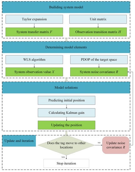
Figure 2.
Flow chart of the fusion positioning algorithm.
3. Experiments and Results
3.1. Experimental Protocol
3.1.1. Experimental Scene
In order to verify the effectiveness of the proposed algorithm, two narrow scenes with different length–width ratios were selected for experimental verification, as shown in Figure 3. Scene A was the dormitory corridor of South China Normal University. The whole experimental scene was 24 m long and 2 m wide. Scene B was the dormitory corridor junction of South China Normal University. The whole experimental scene was 20 m long and 3 m wide.
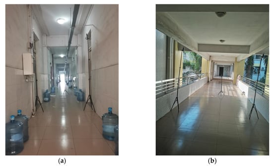
Figure 3.
Experimental scene: (a) corridor; (b) connection of corridors.
3.1.2. Experimental Hardware
The hardware used in this experiment is shown in Figure 4. The bottom plate adopts an STM32F103 series single-chip microcomputer as the main control chip. Peripheral circuits include an LED display, charging interface, etc. The module is configured with DecaWave ‘s DWM1000. The hardware can be configured as a base station or a tag via USB instructions.
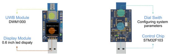
Figure 4.
Hardware architecture of the positioning module.
3.1.3. Experimental Scheme
To systematically explore the DOP distribution characteristics under different narrow space scenes and base station networking and to verify the proposed positioning algorithm, this paper designed the following experimental scheme.
Based on the equations of the DOP numerical analysis model, the model simulation was carried out to explore the geometric configuration relationship between the node to be tested and the base station in the narrow space. Moreover, the DOP values in the wide space were also compared with the narrow space.
Two long and narrow scenes with different geometric structures were selected in this study. The accuracy and stability of the LS positioning algorithm, the WLS positioning algorithm and the fusion positioning algorithm proposed in this paper were analyzed and compared in both static and dynamic modes.
3.2. Experimental Results of the DOP Numerical Analysis Model
In this experiment, the simulated environment is a wide space of 24 × 24 × 3 m, a corridor of 24 × 2 × 3 m and a channel of 20 × 3 × 3 m. The coordinates of the base station in the wide space, corridor space and channel space are shown in Table 1, Table 2 and Table 3. Starting from the origin of the coordinates in the lower left corner (node position to be measured), the whole simulation area was traversed with a step length of 0.1 m. For different simulation scenes, HDOP and PDOP values were calculated by Equations (7) and (8), respectively. The simulation results are shown in Figure 5, Figure 6 and Figure 7.

Table 1.
Base station coordinates in a wide simulation space.
Table 2.
Base station coordinates in a corridor simulation space.
Table 3.
Base station coordinates in a passage simulation space.
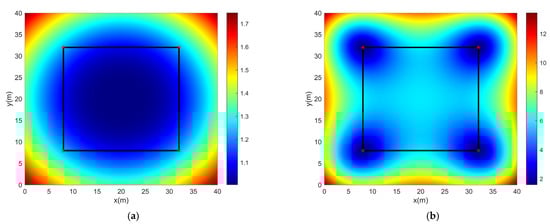
Figure 5.
DOP values in wide simulation space: (a) HDOP values; (b) PDOP values.
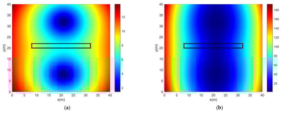
Figure 6.
DOP values in corridor simulation space: (a) HDOP values; (b) PDOP values.
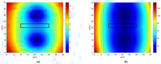
Figure 7.
DOP values in passage simulation space: (a) HDOP values; (b) PDOP values.
It can be seen in Figure 5, Figure 6 and Figure 7 that in a wide space, the PDOP values are basically in the range of 2 to 6, and the HDOP values are not higher than 1.2. The PDOP values of the corridor space are basically in the range of 20 to 80, and the HDOP values are in the range of 6 to 10. In the passage space, the HDOP values are approximately 4, and the PDOP values are in the range of 15 to 20.
According to the experimental results, the DOP value in the narrow space is 10–20 times higher than that in general indoor environments. Such a high DOP value means that there is a very demanding requirement for ranging accuracy in a narrow space, and even a small ranging error can lead to inaccurate positioning. On the contrary, in a general indoor environment, the DOP values are low, and the requirement for ranging accuracy is relatively not very high; thus, UWB has higher positioning accuracy in this environment.
3.3. Experimental Results of Positioning
3.3.1. Static Positioning
In the static positioning experiment, considering that the DOP value of each point in the narrow space was quite different, different points in the space were randomly selected for the experiment. Among them, seven points were selected in Scene A, and eight points were selected in Scene B. The coordinate diagram of the base station and the selected positioning tag is shown in Figure 8.
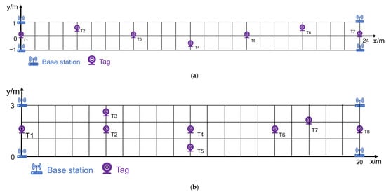
Figure 8.
Base station and tag location map: (a) Scene A; (b) Scene B.
Based on UWB ranging, the ranging values of positioning nodes to different positioning base stations can be obtained. Each positioning node was sampled 200 times. Based on the UWB ranging data, different positioning algorithms were used to yield the position coordinates. Evaluating the performance of a positioning solution is an effective way to improve the performance of a navigation system [46]. The current positioning performance evaluation indicators mainly include root mean square (RMS) error, error cumulative distribution function and Cramér–Rao lower bound [47]. The performance evaluation indices selected in this paper were RMS errors. The RMS errors of the three algorithms at each point are shown in Figure 9 and Figure 10. Table 4 lists the detailed error values.
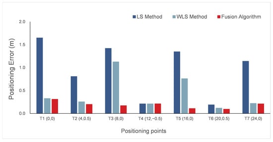
Figure 9.
RMS error of different points in Scene A.
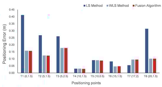
Figure 10.
RMS error of different points in Scene B.
Table 4.
Positioning error of each point in static experiment.
It can be seen from Figure 9 and Figure 10 that the positioning accuracy of the fusion positioning algorithm proposed in this paper was higher than that of the WLS positioning algorithm, and it was much higher than that of the LS positioning algorithm. According to the detailed error values in Table 4, for most points, the proposed fusion algorithm reported the lowest error in both scenes. For Scene A, the mean square error of the LS positioning algorithm was 93.77 cm; the mean square error of the WLS positioning algorithm was 42.94 cm; and the mean square error of the fusion positioning algorithm was 18.67 cm. Compared with the LS positioning algorithm and the WLS positioning algorithm, the fusion positioning algorithm improved the accuracy by 80.1% and 56.5%, respectively. For Scene B, the average positioning error of the LS positioning algorithm was 19.6 cm, and the average positioning error of the WLS positioning algorithm and the fusion positioning algorithm was 10.59 cm, which meets the requirements of high-precision positioning. Compared with the LS positioning algorithm, the fusion positioning algorithm improved the accuracy by 45.9%.
3.3.2. Dynamic Positioning
In the experiment, the handheld tag moved at a constant speed according to the preset trajectory. During this period, the system performed positioning every 0.1 s and stopped data acquisition when it reached the end point. In Scene A, the tag started from (−0.5, 0) and moved around a rectangle with a length of 24 m and a width of 1 m. In Scene B, the tag started at (0.5, 0) and moved around a rectangle with a length of 20 m and a width of 1.5 m. Since the LS method has a poor positioning effect in this space, its positioning was not presented in the report. The positioning results of WLS and the proposed algorithm are shown in Figure 11 and Figure 12. The solid line represents the real trajectory of the moving object.
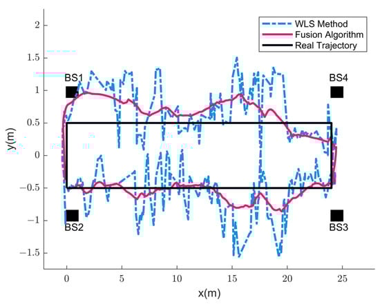
Figure 11.
Dynamic trajectory diagram in Scene A.
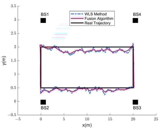
Figure 12.
Dynamic trajectory diagram in Scene B.
According to Figure 11, in Scene A, when the tag position was solved by WLS, the positioning result had a large oscillation, and the positioning trajectory was quite different from the real trajectory. However, when the fusion positioning was used to solve the tag position, the positioning result is smoother and the whole positioning trajectory is roughly consistent with the real trajectory. The calculation showed that the RMS errors of the WLS positioning algorithm and the fusion positioning algorithm were 34.91 and 21.17 cm, respectively. The accuracy of the fusion positioning algorithm was 39.36% higher than that of the WLS positioning algorithm.
According to Figure 12, in Scene B, whether WLS or the fusion positioning algorithm were used to solve the tag position, the positioning results of the two were not much different, and both trajectories fit well with the real trajectory. The RMS errors of the WLS positioning algorithm and the fusion positioning algorithm were 11.25 and 10.34 cm, respectively. In this scene, the average accuracy of the fusion positioning algorithm was 8.09% higher than that of the WLS positioning algorithm.
4. Discussion
In this study, an indoor positioning algorithm combining DOP and KF was proposed for the narrow space. Comparative experiments were carried out on different scenes and different algorithms. The algorithm was also tested in both static and dynamic terms. The following will discuss the characteristics of DOP in a narrow space and the reasons behind the positioning results.
In the experiments of DOP numerical analysis model, the DOP values of different scenes were compared. We found that the DOP values in a narrow space were much higher than that in a wide space. This phenomenon was consistent with some existing research reports [48,49]. In general, a PDOP value of 3 or less and an HDOP value of 1 or less indicate a good base station layout [50], where the positioning solution can meet the requirements of high-precision positioning [8]. However, in a narrow corridor, the angles between the tag and different base stations are quite close, resulting in small unit vector geometry [16]. Under this circumstance, the small ranging error will cause great positioning error. Therefore, the UWB positioning accuracy of a narrow space will become very low.
In the positioning experiments, the positioning results of three algorithms in different narrow scenes were compared. The fusion algorithm had better positioning accuracy and stability than the other two algorithms. According to the DOP numerical analysis experimental results and existing research conclusions [16], in the narrow space, the positioning error mainly comes from the special spatial structure of the space (the DOP values are high). Since the DOP values reflect the influence of the ranging error on the positioning accuracy, the larger DOP values mean that it is easy to introduce more noise during positioning [51]. However, previous studies have only improved the positioning accuracy from the perspective of the algorithm, ignoring the impact of the scene itself [52,53]. Through the DOP experiments on different scenes and the parameter analysis on KF, we found that the DOP values were positively correlated with the observation noise parameter value of KF. Therefore, this study contributed to the existing studies and tried to adaptively introduce the DOP values of the target scene into KF. According to the experimental results in both static and dynamic terms, the proposed method adaptively suppressed the error by introducing the DOP values into the KF algorithm.
Furthermore, we try to explain some specific phenomena in the two positioning experiments. In the static positioning experiments, for the T4 point in Figure 8, the positioning accuracy of the three algorithms was basically the same, and the positioning error of T4 point was far lower than that of other points. This was because T4 was closer to the center point; thus, the weight of the WLS was not much different from that of the LS at this time, and thus, the positioning results of the two algorithms were basically the same. Furthermore, the fusion algorithm was improved on the basis of WLS, and the DOP value at T4 is relatively small. The phenomenon further proves that the proposed algorithm is more likely to improve the positioning accuracy for the points with higher DOP values. In the dynamic positioning experiment, in Scene A, when the tag position was solved by WLS, the positioning trajectory was not consistent with the real trajectory and produced large oscillation. This was because the value distribution of DOP in this scene was very large, and even a small ranging error would cause a serious positioning error. Meanwhile, in a confined space such as Scene A, there was a large amount of reflection and diffraction of electromagnetic wave propagation, thus causing a serious multipath effect [14,15]. This degraded the ranging performance of UWB [54]. As a result, the trajectory obtained by WLS solution at this time differed greatly from the real trajectory. However, when the fusion algorithm was used to solve the tag position, the trajectory was much better than the WLS result. This was because the fusion algorithm combined the DOP numerical analysis model to improve the algorithm. Thus, the negative influence of the high DOP values in this scene was automatically suppressed by the fusion algorithm. However, due to the problem of ranging error, there were still some errors between the positioning trajectory obtained by this method and the real trajectory. In Scene B, the results obtained by WLS and the fusion positioning algorithm were basically the same and quite fitted the real trajectory. This was because the DOP in this scene was relatively small, and the whole space was transparent. There was less reflection and diffraction in the propagation of electromagnetic waves. Consequently, both algorithms had good positioning accuracy in this scene. These phenomena indicated that the algorithm proposed in this paper was not only suitable for the airtight narrow space, but also for general indoor environment.
In general, although the spatial structure of Scene A and Scene B was different, the accuracy of the algorithm proposed in this paper had different degrees of improvement in both scenes, especially in the scene with the higher DOP values (scene A). It can be seen that the proposed positioning method improved the accuracy more in the narrower space.
5. Conclusions
UWB technology has attracted attention because of its high-precision ranging, but conventional positioning algorithms based on UWB technology have large positioning errors in the narrow space. This study contributed to the existing research and designed a fusion algorithm by combining DOP and KF for UWB positioning in a narrow space. In the proposed algorithm, the DOP numerical analysis model and the WLS positioning results were used as measurement noise covariance and observation of KF, respectively. The algorithm was tested on two scenes with different length–width ratios. Both static and dynamic positioning experiments were designed on the scenes to compare the proposed algorithm and other algorithms. The experimental results showed that the fusion positioning algorithm proposed in this paper had an evident higher positioning accuracy in a narrow space compared with the traditional algorithms. From the detailed analysis of the results, we found that the higher the DOP values of the scene, the greater the accuracy improvement of the algorithm. The main reason was that the positioning error was adaptively suppressed after the DOP values of the target scene was fused.
However, this study only took line-of-sight conditions as the experimental environment to verify the feasibility of the proposed method. Meanwhile, we only considered a single sensor (UWB) and chose a more conventional Kalman filter for the data fusion process. In future research, it will be necessary to further examine the performance of the proposed algorithm in a NLOS environment and integrate a localization pattern. Furthermore, we can try to use a combination of extended Kalman filtering and DOP numerical analysis models to accomplish the data processing.
Author Contributions
Conceptualization, Y.G. and G.Y.; methodology, G.Y. and Z.J.; validation, Y.G. and J.Y.; formal analysis, Y.G., G.Y. and W.L.; data curation, Y.G. and J.Y.; writing—original draft preparation, Y.G.; writing—review and editing, G.Y. and W.L.; visualization, Y.G.; supervision, G.Y.; project administration, W.L.; funding acquisition, W.L. All authors have read and agreed to the published version of the manuscript.
Funding
This research was funded by the Ministry of Science and Technology of the People’s Republic of China, grant number (2020YFF0303604), and in part by the Guangzhou Association for Science and Technology, grant number (20200115-8).
Data Availability Statement
The data that support the findings of this study are available from the corresponding author, Y.G., upon reasonable request.
Conflicts of Interest
The authors declare no conflict of interest.
References
- Oguntala, G.; Abd-Alhameed, R.; Jones, S.; Noras, J.; Patwary, M.; Rodriguez, J. Indoor Location Identification Technologies for Real-Time IoT-Based Applications: An Inclusive Survey. Comput. Sci. Rev. 2018, 30, 55–79. [Google Scholar] [CrossRef]
- Zafari, F.; Gkelias, A.; Leung, K.K. A Survey of Indoor Localization Systems and Technologies. IEEE Commun. Surv. Tutor. 2019, 21, 2568–2599. [Google Scholar] [CrossRef]
- Asaad, S.M.; Maghdid, H.S. A Comprehensive Review of Indoor/Outdoor Localization Solutions in IoT Era: Research Challenges and Future Perspectives. Comput. Netw. 2022, 212, 109041. [Google Scholar] [CrossRef]
- Zhuang, Y.; Wang, Q.; Shi, M.; Cao, P.; Qi, L.; Yang, J. Low-Power Centimeter-Level Localization for Indoor Mobile Robots Based on Ensemble Kalman Smoother Using Received Signal Strength. IEEE Internet Things J. 2019, 6, 6513–6522. [Google Scholar] [CrossRef]
- Otero, R.; Lagüela, S.; Garrido, I.; Arias, P. Mobile Indoor Mapping Technologies: A Review. Autom. Constr. 2020, 120, 103399. [Google Scholar] [CrossRef]
- Maranò, S.; Gifford, W.M.; Wymeersch, H.; Win, M.Z. NLOS Identification and Mitigation for Localization Based on UWB Experimental Data. IEEE J. Sel. Areas Commun. 2010, 28, 1026–1035. [Google Scholar] [CrossRef]
- Alarifi, A.; Al-Salman, A.; Alsaleh, M.; Alnafessah, A.; Al-Hadhrami, S.; Al-Ammar, M.A.; Al-Khalifa, H.S. Ultra Wideband Indoor Positioning Technologies: Analysis and Recent Advances. Sensors 2016, 16, 707. [Google Scholar] [CrossRef]
- Chandra, A.; Prokeš, A.; Mikulášek, T.; Blumenstein, J.; Kukolev, P.; Zemen, T.; Mecklenbräuker, C.F. Frequency-Domain In-Vehicle UWB Channel Modeling. IEEE Trans. Veh. Technol. 2016, 65, 3929–3940. [Google Scholar] [CrossRef]
- Wang, S.; Mao, G.; Zhang, J.A. Joint Time-of-Arrival Estimation for Coherent UWB Ranging in Multipath Environment with Multi-User Interference. IEEE Trans. Signal Process. 2019, 67, 3743–3755. [Google Scholar] [CrossRef]
- Zhao, Y.; Wang, M. The LOS/NLOS Classification Method Based on Deep Learning for the UWB Localization System in Coal Mines. Appl. Sci. 2022, 12, 6484. [Google Scholar] [CrossRef]
- Yu, B.; Fan, G.; Luo, Y.; Sheng, C.; Gan, X.; Huang, L.; Rong, Q. Multi-Source Fusion Positioning Algorithm Based on Pseudo-Satellite for Indoor Narrow and Long Areas. Adv. Space Res. 2021, 68, 4456–4469. [Google Scholar] [CrossRef]
- Zhao, W.; Zong, R.; Yao, B.; Gao, J.; Liao, G. Analysis of Influencing Factors on Flashover in the Long-Narrow Confined Space. Procedia Eng. 2013, 62, 250–257. [Google Scholar] [CrossRef]
- Sadeghi, S.; Soltanmohammadlou, N.; Nasirzadeh, F. Applications of Wireless Sensor Networks to Improve Occupational Safety and Health in Underground Mines. J. Safety Res. 2022, in press. [Google Scholar] [CrossRef]
- Ranjan, A.; Sahu, H.B.; Misra, P. Modeling and Measurements for Wireless Communication Networks in Underground Mine Environments. Measurement 2020, 149, 106980. [Google Scholar] [CrossRef]
- Sharp, I.; Yu, K.; Hedley, M. On the GDOP and Accuracy for Indoor Positioning. IEEE Trans. Aerosp. Electron. Syst. 2012, 48, 2032–2051. [Google Scholar] [CrossRef]
- Jian, S.; Yongling, F.; Lin, T.; Shengguang, L. A Survey and Application of Indoor Positioning Based on Scene Classification Optimization. In Proceedings of the 2015 IEEE 12th Intl Conf on Ubiquitous Intelligence and Computing and 2015 IEEE 12th Intl Conf on Autonomic and Trusted Computing and 2015 IEEE 15th Intl Conf on Scalable Computing and Communications and Its Associated Workshops (UIC-ATC-ScalCom), Beijing, China, 10–14 August 2015; pp. 1558–1562. [Google Scholar]
- Wang, H.; Zhan, X.; Zhang, Y. Geometric Dilution of Precision for GPS Single-Point Positioning Based on Four Satellites. J. Syst. Eng. Electron. 2008, 19, 1058–1063. [Google Scholar] [CrossRef]
- Li, C.; Teng, Y.; Kang, R. Some Remarks on Geometric Dilution of Precision (GDOP) at User Level in Multi-GNSS Positioning. Adv. Space Res. 2018, 62, 3048–3052. [Google Scholar] [CrossRef]
- Feng, G.; Shen, C.; Long, C.; Dong, F. GDOP Index in UWB Indoor Location System Experiment. In Proceedings of the 2015 IEEE Sensors, Valencia, Spain, 1–4 November 2015; pp. 1–4. [Google Scholar]
- Wang, M.; Chen, Z.; Zhou, Z.; Fu, J.; Qiu, H. Analysis of the Applicability of Dilution of Precision in the Base Station Configuration Optimization of Ultrawideband Indoor TDOA Positioning System. IEEE Access 2020, 8, 225076–225087. [Google Scholar] [CrossRef]
- Bais, A.; Kiwan, H.; Morgan, Y. On Optimal Placement of Short Range Base Stations for Indoor Position Estimation. J. Appl. Res. Technol. 2014, 12, 886–897. [Google Scholar] [CrossRef]
- Syafrudin, M.; Walter, C.; Schweinzer, H. Robust Locating Using LPS LOSNUS under NLOS Conditions. In Proceedings of the 2014 International Conference on Indoor Positioning and Indoor Navigation (IPIN), Busan, Korea, 27–30 October 2014; pp. 582–590. [Google Scholar]
- Auger, F.; Hilairet, M.; Guerrero, J.M.; Monmasson, E.; Orlowska-Kowalska, T.; Katsura, S. Industrial Applications of the Kalman Filter: A Review. IEEE Trans. Ind. Electron. 2013, 60, 5458–5471. [Google Scholar] [CrossRef]
- Basar, T. A New Approach to Linear Filtering and Prediction Problems. In Control Theory: Twenty-Five Seminal Papers (1932–1981); IEEE: Piscataway, NJ, USA, 2001; pp. 167–179. ISBN 978-0-470-54433-4. [Google Scholar]
- Janjanam, L.; Saha, S.K.; Kar, R.; Mandal, D. Improving the Modelling Efficiency of Hammerstein System Using Kalman Filter and Its Parameters Optimised Using Social Mimic Algorithm: Application to Heating and Cascade Water Tanks. J. Frankl. Inst. 2022, 359, 1239–1273. [Google Scholar] [CrossRef]
- Li, Q.; Li, R.; Ji, K.; Dai, W. Kalman Filter and Its Application. In Proceedings of the 2015 8th International Conference on Intelligent Networks and Intelligent Systems (ICINIS), Tianjin, China, 1–3 November 2015; pp. 74–77. [Google Scholar]
- Li, M. The Simulation Research of Multi-Model Adaptive KF and Target Tracking. In Proceedings of the 2021 Chinese Intelligent Systems Conference; Jia, Y., Zhang, W., Fu, Y., Yu, Z., Zheng, S., Eds.; Springer: Singapore, 2022; pp. 11–18. [Google Scholar]
- Li, D.; Wang, X.; Chen, D.; Zhang, Q.; Yang, Y. A Precise Ultra-Wideband Ranging Method Using Pre-Corrected Strategy and Particle Swarm Optimization Algorithm. Measurement 2022, 194, 110966. [Google Scholar] [CrossRef]
- Zhao, L.; Wang, R.; Wang, J.; Yu, T.; Su, A. Nonlinear State Estimation with Delayed Measurements Using Data Fusion Technique and Cubature Kalman Filter for Chemical Processes. Chem. Eng. Res. Des. 2019, 141, 502–515. [Google Scholar] [CrossRef]
- Liu, F.; Liu, Y.; Sun, X.; Sang, H. A New Multi-Sensor Hierarchical Data Fusion Algorithm Based on Unscented Kalman Filter for the Attitude Observation of the Wave Glider. Appl. Ocean Res. 2021, 109, 102562. [Google Scholar] [CrossRef]
- Cheng, J.H.; Yu, P.P.; Huang, Y.R. Application of Improved Kalman Filter in Under-Ground Positioning System of Coal Mine. IEEE Trans. Appl. Supercond. 2021, 31, 0603904. [Google Scholar] [CrossRef]
- Feng, D.; Wang, C.; He, C.; Zhuang, Y.; Xia, X.-G. Kalman-Filter-Based Integration of IMU and UWB for High-Accuracy Indoor Positioning and Navigation. IEEE Internet Things J. 2020, 7, 3133–3146. [Google Scholar] [CrossRef]
- Ananthasayanam, M.R.; Mohan, M.S.; Naik, N.; Gemson, R.M.O. A Heuristic Reference Recursive Recipe for Adaptively Tuning the Kalman Filter Statistics Part-1: Formulation and Simulation Studies. Sādhanā 2016, 41, 1473–1490. [Google Scholar] [CrossRef]
- Zhang, X.; Ding, F.; Xu, L.; Yang, E. Highly Computationally Efficient State Filter Based on the Delta Operator. Int. J. Adapt. Control Signal Process. 2019, 33, 875–889. [Google Scholar] [CrossRef]
- Tabacek, J.; Havlena, V. Reduction of Prediction Error Sensitivity to Parameters in Kalman Filter. J. Frankl. Inst. 2022, 359, 1303–1326. [Google Scholar] [CrossRef]
- Herrera, L.; Rodríguez-Liñán, M.C.; Clemente, E.; Meza-Sánchez, M.; Monay-Arredondo, L. Evolved Extended Kalman Filter for First-Order Dynamical Systems with Unknown Measurements Noise Covariance. Appl. Soft Comput. 2022, 115, 108174. [Google Scholar] [CrossRef]
- Wang, J.; Ying, J.; Jiang, S. UWB Base Station Layout Optimization in Underground Parking Lots. J. Highw. Transp. Res. Dev. Engl. Ed. 2021, 15, 82–87. [Google Scholar] [CrossRef]
- Xiaolin, N.; Yuqing, Y.; Mingzhen, G.; Weiren, W.; Jiancheng, F.; Gang, L. Pulsar Navigation Using Time of Arrival (TOA) and Time Differential TOA (TDTOA). Acta Astronaut. 2018, 142, 57–63. [Google Scholar] [CrossRef]
- Zhang, Y.; Chu, Y.; Fu, Y.; Li, Z.; Song, Y. UWB Positioning Analysis and Algorithm Research. Procedia Comput. Sci. 2022, 198, 466–471. [Google Scholar] [CrossRef]
- Xu, P. Improving the Weighted Least Squares Estimation of Parameters in Errors-in-Variables Models. J. Frankl. Inst. 2019, 356, 8785–8802. [Google Scholar] [CrossRef]
- Svecova, M.; Kocur, D.; Zetik, R. Object Localization Using Round Trip Propagation Time Measurements. In Proceedings of the 2008 18th International Conference Radioelektronika, Prague, Czech Republic, 24–25 April 2008; pp. 1–4. [Google Scholar]
- Biswas, S.K.; Qiao, L.; Dempster, A.G. Effect of PDOP on Performance of Kalman Filters for GNSS-Based Space Vehicle Position Estimation. GPS Solut. 2017, 21, 1379–1387. [Google Scholar] [CrossRef]
- Navon, E.; Bobrovsky, B.Z. An Efficient Outlier Rejection Technique for Kalman Filters. Signal Process. 2021, 188, 108164. [Google Scholar] [CrossRef]
- Wang, G.; Chen, B.; Yang, X.; Peng, B.; Feng, Z. Numerically Stable Minimum Error Entropy Kalman Filter. Signal Process. 2021, 181, 107914. [Google Scholar] [CrossRef]
- Liu, T.; Cheng, S.; Wei, Y.; Li, A.; Wang, Y. Fractional Central Difference Kalman Filter with Unknown Prior Information. Signal Process. 2019, 154, 294–303. [Google Scholar] [CrossRef]
- Qiu, F.; Zhang, W. Position Error vs. Signal Measurements: An Analysis towards Lower Error Bound in Sensor Network. Digit. Signal Process. 2022, 129, 103637. [Google Scholar] [CrossRef]
- Zheng, X.; Liu, H.; Yang, J.; Chen, Y.; Martin, R.P.; Li, X. A Study of Localization Accuracy Using Multiple Frequencies and Powers. IEEE Trans. Parallel Distrib. Syst. 2014, 25, 1955–1965. [Google Scholar] [CrossRef]
- Sharma, R.; Badarla, V. Geometrical Optimization of A Novel Beacon Placement Strategy for 3D Indoor Localization. In Proceedings of the 2018 IEEE International Conference on Advanced Networks and Telecommunications Systems (ANTS), Indore, India, 16–19 December 2018; pp. 1–6. [Google Scholar]
- Pan, H.; Qi, X.; Liu, M.; Liu, L. Indoor Scenario-Based UWB Anchor Placement Optimization Method for Indoor Localization. Expert Syst. Appl. 2022, 205, 117723. [Google Scholar] [CrossRef]
- Specht, M. Experimental Studies on the Relationship between HDOP and Position Error in the GPS System. Metrol. Meas. Syst. 2022, 29, 17–36. [Google Scholar]
- Li, Y.; Zhang, Z.; He, X.; Wen, Y.; Cao, X. Realistic Stochastic Modeling Considering the PDOP and Its Application in Real-Time GNSS Point Positioning under Challenging Environments. Measurement 2022, 197, 111342. [Google Scholar] [CrossRef]
- Djosic, S.; Stojanovic, I.; Jovanovic, M.; Djordjevic, G.L. Multi-Algorithm UWB-Based Localization Method for Mixed LOS/NLOS Environments. Comput. Commun. 2022, 181, 365–373. [Google Scholar] [CrossRef]
- Li, C.T.; Cheng, J.C.P.; Chen, K. Top 10 Technologies for Indoor Positioning on Construction Sites. Autom. Constr. 2020, 118, 103309. [Google Scholar] [CrossRef]
- Yu, K.; Wen, K.; Li, Y.; Zhang, S.; Zhang, K. A Novel NLOS Mitigation Algorithm for UWB Localization in Harsh Indoor Environments. IEEE Trans. Veh. Technol. 2019, 68, 686–699. [Google Scholar] [CrossRef]


Publisher’s Note: MDPI stays neutral with regard to jurisdictional claims in published maps and institutional affiliations. |
© 2022 by the authors. Licensee MDPI, Basel, Switzerland. This article is an open access article distributed under the terms and conditions of the Creative Commons Attribution (CC BY) license (https://creativecommons.org/licenses/by/4.0/).