Abstract
Most high-performance semantic segmentation networks are based on complicated deep convolutional neural networks, leading to severe latency in real-time detection. However, the state-of-the-art semantic segmentation networks with low complexity are still far from detecting objects accurately. In this paper, we propose a real-time semantic segmentation network, RecepNet, which balances accuracy and inference speed well. Our network adopts a bilateral architecture (including a detail path, a semantic path and a bilateral aggregation module). We devise a lightweight baseline network for the semantic path to gather rich semantic and spatial information. We also propose a detail stage pattern to store optimized high-resolution information after removing redundancy. Meanwhile, the effective feature-extraction structures are designed to reduce computational complexity. RecepNet achieves an accuracy of 78.65% mIoU (mean intersection over union) on the Cityscapes dataset in the multi-scale crop and flip evaluation. Its algorithm complexity is 52.12 GMACs (giga multiply–accumulate operations) and its inference speed on an RTX 3090 GPU is 50.12 fps. Moreover, we successfully applied RecepNet for blue-green algae real-time detection. We made and published a dataset consisting of aerial images of water surface with blue-green algae, on which RecepNet achieved 82.12% mIoU. To the best of our knowledge, our dataset is the world’s first public dataset of blue-green algae for semantic segmentation.
1. Introduction
Semantic segmentation is a computer vision task that assigns pixel-level labels to images. It is widely used in scene understanding [1], automotive driving [2] and video surveillance [3]. These applications require real-time interaction, so they have a strong demand for inference speed and accuracy.
Generally, to achieve superior accuracy, most semantic segmentation networks rely on complex baseline deep convolutional neural networks (DCNNs) [4] such as VGG [4], ResNet [5] and Xception [6]. These baseline networks usually consist of hundreds of layers and expand the input into thousands of channels. Therefore, they have high computational complexity and memory burden, leading to poor inference speed. For example, deeplabv3+ [6] takes more than one second to infer on a high-resolution image, even using a high-performance GPU. Due to the increasing demand for real-time detection, fast semantic segmentation methods are beginning to develop, such as Enet [7] and SegNet [8]. These methods can serve for real-time inference with low latency. However, their accuracy is unsatisfactory because the features are not fully learned. Therefore, making a good trade-off between two seemingly contradictory terms—accuracy and speed—is a critical and challenging problem. Recently, with the rapid development of semantic segmentation, many state-of-the-art works have made great efforts on effective models and backbone architectures, trying to increase the accuracy while keeping the complexity cost as small as possible. Traditionally, an encoder–decoder backbone uses a top-down structure and lateral connections to recover spatial features that are destroyed in the downsampling process [9]. However, numerous connections in the structure bring a heavy memory burden. The bilateral architecture is proposed in the bilateral segmentation network (BiSeNetV2) [10], with one path storing spatial details and another gathering categorical semantics. BiSeNetV2 uses a lightweight network in the semantic path for real-time inference. However, it is still far behind in terms of detection accuracy.
We observed that enlarging the receptive field of the network is critical to improving accuracy. Generally, the receptive field refers to the sub-region size of the image involved in the convolutional operation, and a larger receptive field provides more contextual information. However, feature representation needs not only semantic information, but also spatial information, which is stored in image channels when the image size is shrunk. Therefore, in the feature-extraction process, it is essential to enlarge the receptive field in both semantic and spatial dimensions.
To pursue better accuracy while maintaining low complexity, we propose a network with a large receptive field (RecepNet) for real-time semantic segmentation. In RecepNet, we adopt a bilateral segmentation backbone, which consists of a detail path storing spatial information, a semantic path extracting semantic information, an aggregation module integrating the two paths and a training booster to enhance the features in the training phases. For the semantic path, we designed lightweight baseline networks consisting of gather–expand–search (GES) layers. This mainly consists of two bottlenecks: a gather-and-expansion bottleneck to downsample with a large spatial receptive field and search-space bottlenecks to search for contextual information in a large receptive field. Efficient convolution operations are used to reduce the complexity. For the stages in the detail path, we designed a detail stage pattern: a fast downsample to preserve useful information in the spatial dimension and then further optimize semantic feature representation.
Our contributions are summarized as follows:
- We propose an effective stem block. It is used in both the detail path and semantic path for fast downsampling while expanding channels flexibly;
- Gather–expand–search (GES) layer, a lightweight downsampling network, is proposed for the semantic path to achieve fast and robust feature extraction. It obtains rich spatial and semantic information by gathering the semantic features, expanding to large dimensions, and searching for multi-resolution features;
- We design a detail stage pattern. It cleans the redundant information, reserves the high-resolution information in the spatial dimension, and improves feature representation;
- A novel training boosting strategy is devised. It improves accuracy by strengthening and recalibrating features in the training phases.
Our network achieves impressive results on the benchmark dataset, Cityscapes. The accuracy of the multi-scale crop and flip evaluation is mIoU (mean intersection over union), and the algorithm complexity is 52.12 GMACs (giga multiply–accumulate operations). Compared with BiSeNetV2, our network improves the accuracy significantly (+ mIoU) with a minor increase in complexity (+0.4 GMACs); compared with Deeplabv3+, our network reduces the complexity significantly (−3.4 GMACs), though the accuracy is slightly brought down (− mIoU). Experimental results show that RecepNet can infer more than 50 images per second on an RTX3090 graphics card, which can process live video in real-time.
We also apply RecepNet on massive UAV photos to automatically detect blue-green algae on a lake surface to monitor its outbreak. We created a blue-green algae set with 1305 images, which, to the best of our knowledge, is the first public blue-green algae set for semantic segmentation. In the work, experimental results show that our algorithm can obtain an 82.12% mIoU.
2. Literature Review
Traditional semantic segmentation methods utilize hand-crafted features, such as the threshold selection [11], random forest [12], boosting [13] and super-pixel [14]. However, the performance of these methods is far from satisfactory. In recent years, semantic segmentation has achieved significant advances by applying DCNNs [15].
2.1. High-Performance Semantic Segmentation
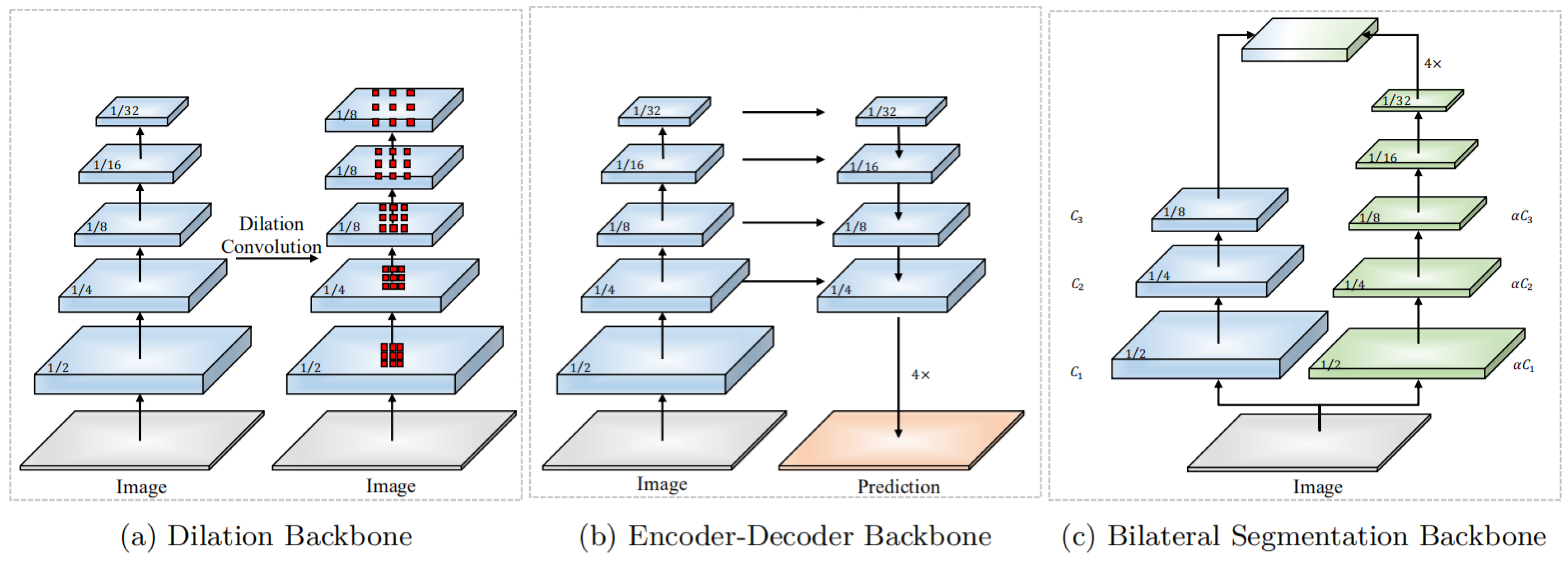
The predecessor of applying DCNNs in semantic segmentation is the fully convolutional network (FCN) [16]. It removes the last fully-connected layers in a DCNN. The later semantic segmentation methods keep improving based on the FCN. These successors mainly can be categorized into three types of architectures: (a) dilation backbone; (b) encoder–decoder backbone; (c) bilateral segmentation backbone. Their structures are shown in Figure 1 [10].
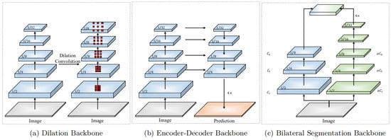
Figure 1.
Three types of backbone. (a), Dilation Backbone; (b), Encoder-Decoder Backbone; (c), Bilateral Segmentation Backbone. Graph from Changqian Yu, BiSeNet V2: Bilateral Network with Guided Aggregation for Real-time Semantic Segmentation [10].
The originator of the dilation backbone is DeepLab [17], which designs the atrous convolution. It limits the downsampling rate to 16 and applies Atrous convolution to extract features further. This design can preserve high-resolution features and expand the receptive field of the network. DeepLabv2 [18] further develops the atrous spatial pyramid pooling (ASPP) module. It has multiple parallel branches with different atrous rates to integrate multi-resolution features. Meanwhile, PSPNet [19] also applies pyramid pooling on the dilation backbone. Some methods also combine with attention mechanisms to capture long-range semantic information, such as self-attention [20] and channel attention [21].
The representative work of encoder–decoder backbones is U-Net [22]. It adopts a top-down architecture to downsample (encoder) and utilizes lateral connections to recover high-resolution features (decoder). The development of the encoder–decoder backbone includes RefineNet [9], which proposed multi-path refinement, DFN [23], which embeds channel attention module to help with recovering features, and HRNet [24], which designs multi-branches to retain high-resolution features. Some algorithms also adopt conditional random fields (CRF) [25] to optimize the accuracy of object boundaries.
The third type of backbone is the bilateral segmentation backbone, which is proposed by bilateral segmentation network (BiSeNetV2) [10]. This kind of architecture consists of two pathways; one is responsible for reserving spatial details (high-resolution features) and the other is for extracting categorical semantics (low-resolution features). The two types of output features are integrated at the end of the network. This design leads to effective real-time semantic segmentation with high accuracy.
2.2. Real-Time Semantic Segmentation
Real-time inference requires a network response with high-quality results as fast as possible. In recent years, many works have made progress in increasing the inference speed. Enet [7] takes the lead in making significant progress in real-time semantic segmentation. It constructs a lightweight network from the script, adapting the encoder–decoder architecture. On the base of Enet, ESPNet [26] using spatial pyramid module and ERFNet [27] using residual connections further improve the accuracy with similar speed. Later on, ICNet [28] simplifies the PSPNet [19] and combines a cascade framework, achieving a good accuracy for high-resolution images. However, ICNet has poor performance for low-resolution images. LEDNet [29], an encoder–decoder-based network, introduces channel split and shuffle to accelerate inference speed. Recently, BiSeNetV2 proposed a bilateral architecture to balance accuracy and speed.
Additionally, some lightweight structures are proposed to reduce the complexity of the network, such as MobileNet [30] and ShuffleNet [31]. Recently, FasterSeg [32] devised zoomed convolution to optimize the convolution operation, which consists of bilinear downsampling, standard convolution and bilinear upsampling. According to [32], the zoomed convolution reduces 40% latency and 75% FLOP of standard convolution, which performs better than group convolution (i.e., depth-wise convolution) and atrous convolution.
BeSeNetV2 proposed a two-pathway architecture that significantly improves the performance of real-time semantic segmentation. In the BiSeNetV2, two different branches are responsible for spatial detail information and categorical segmentation information, respectively [10]. There are mainly three parts in this structure. (i) The detail branch uses wide channels to encode rich spatial information. Meanwhile, the detail branch adopts a shallow structure, since a deep network with wide channels brings heavy computation complexity and memory overload. This branch mainly follows the VGG nets. The output feature map of the detail branch is 1/8 of the original input with 128 channels. (ii) The semantic branch uses deep layers and a large receptive field to generate high-level features. To realize real-time recognition, this branch uses a lightweight network. (iii) The detail branch has low-level feature output, while the semantic branch has high-level. The bilateral guided aggregation layer is designed to merge these different scale feature representations, allowing them to communicate efficiently.
3. Methodology
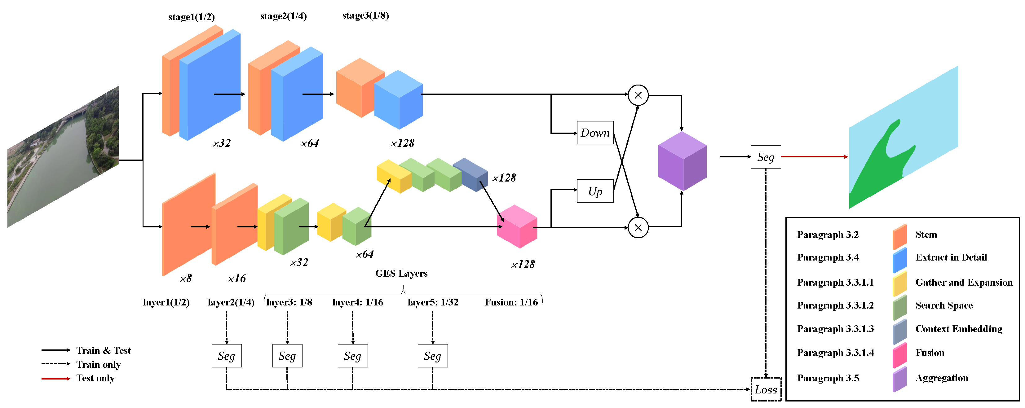
In this paper, we proposed a new semantic segmentation network: RecepNet. RecepNet aims to increase accuracy while reducing complexity. The overall structure and blocks are illustrated in detail in Figure 2 and Table 1 and Table 2.
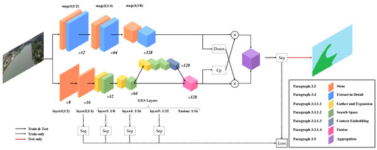
Figure 2.
Overall architecture of RecepNet.

Table 1.
Illustration of instantiation of the Detail Branch Each layer contains one or more operations (SepConv: depth-wise separable convolution). Each operation (opr) has a kernel size k, stride s, output channels c and a downsampling rate.

Table 2.
Illustration of instantiation of the Semantic Branch. Each layer contains one or more operations (GES: gather–expand–search layer; GE: gather-and-expand bottleneck; SS: search-space bottleneck; CE: context embedded block; Fusion: feature fusion block). Each operation (opr) has a kernel size k, stride s, output channels c and a downsampling rate.
3.1. Overview
3.1.1. Core Concept of RecepNet
Enlarging the receptive field when extracting features is crucial to improving accuracy. Generally, the receptive field refers to the subregion’s size on the image involved in the convolutional computation. A large receptive field can provide rich semantic information for feature representation. For example, we can enlarge the receptive field by integrating multi-resolution feature maps. However, for the accuracy of feature representation, the perception ability of spatial information is also essential. The “receptive field” for spatial information is also expected to be enlarged. We can expand the feature map to a higher dimension to achieve this. Enlarging the receptive field for both semantic and spatial information is a crucial concept for RecepNet. In addition, as RecepNet is a real-time network, low latency is another essential criterion for its performance. Therefore, in each component design of RecepNet, we proposed several approaches to reduce the complexity.
3.1.2. Overall Structure
RecepNet adopts BiSeNetV2’s two-pathway architecture. It consists of (1) a semantic path for contextual information, including stem block, gather–expand–search (GES) layers, and context embedded (CE) block; (2) a detail path for spatial information that is composited of a stem block and other convolution operations; (3) a bilateral guided aggregation module to fuse two paths’ outputs; and (4) a training booster strategy to recalibrate the feature representation in the training phases.
3.1.3. Block Design
The two paths consist of various blocks to achieve a large receptive field in both the semantic dimension and spatial dimension, and keep low complexity simultaneously. These well-designed blocks shown in Figure 2 include (1) a stem block, responsible for fast downsampling in both detail path and semantic path, and (2) a gather–expand–search (GES) layer, which is the lightweight downsampling network of Semantic Path. It obtains rich spatial and semantic information by gathering the semantic features, expanding to large dimensions, and searching for multi-resolution features. The GES layer mainly consists of a gather-and-expansion (GE) bottleneck for downsampling and search-space bottlenecks (SS) to search for semantics. The gather-and-expansion bottleneck enlarges the spatial receptive field, while the search-space bottlenecks enlarge the semantic receptive field. The cooperation of two bottlenecks improves the accuracy of feature representation and reduces complexity. (3) A feature fusion block is at the end of the GES layer. It fuses the outputs of the last two layers of the semantic path to enhance the feature representation ability. (4) Finally, there is the context-embedding (CE) block. We adopt the CE block in BiSeNetV2 directly to remedy global information in Layer 5 of the GES layer (with a downsampling rate of 32).
The upper path is the detail path and the bottom path is the semantic path. The detail path consists of Stages 1, 2 and 3. The semantic path consists of Layers 1, 2, 3, 4 and 5, and a fusion layer. Especially, Layers 3, 4 and 5 and the fusion layer constitute the gather–expand–search (GES) layer. The outputs of two paths are aggregated using bilateral guided aggregation. The network blocks are shown in the legend. Stem denotes stem block; Extract in Detail denotes feature-extraction operations in the detail path; GE denotes gather-and-expansion bottleneck; SS denotes search-space bottleneck; CE denotes context-embedding block; Fusion denotes feature fusion flock; Aggregation denotes bilateral aggregation module. Additionally, Seg head is the booster training strategy used in the training phases. Note that in 1 / {2, 4, 8, 16, 32}, the denominators denote the downsampling rate and ×8, 16, 32, 64, 128 denote the output channels.
3.2. Stem Block
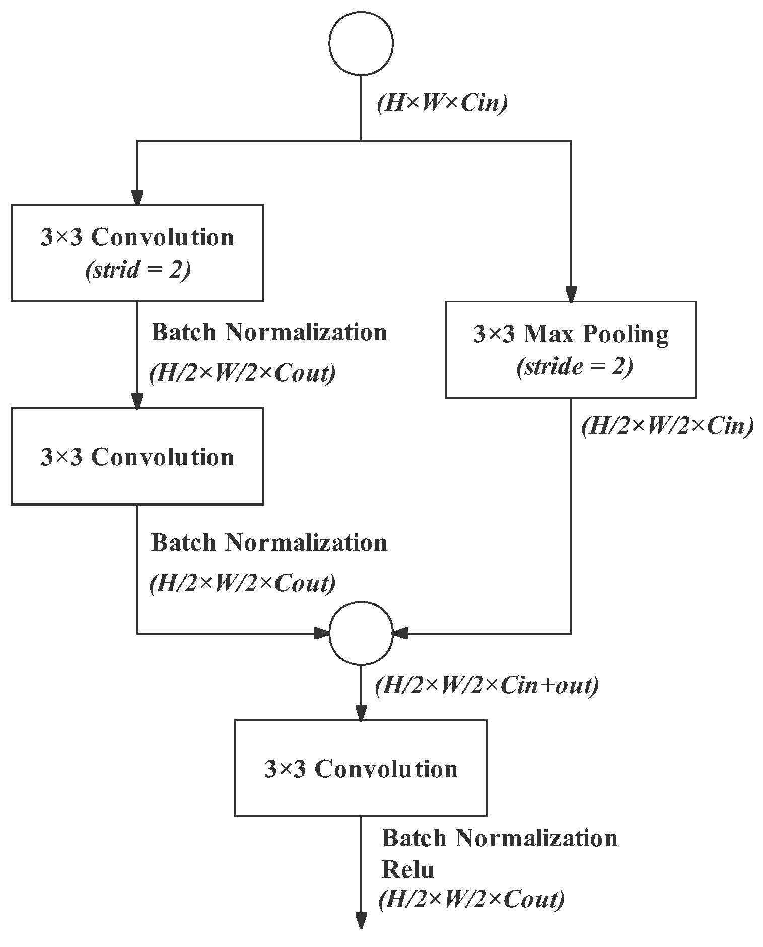
The stem block aims to quickly downsample the input feature map by 1/2 while increasing the number of channels. Inspired by Enet [7], we combine two downsampling methods. As shown in Figure 3, the left branch is two successive 3 × 3 convolutions. The first one (stride of 2) shrinks the image size while expanding the channels to the number of output channels, and the second one strengthens the feature representation. Each convolution operation is only followed by a batch normalization because an activation function here will reduce the accuracy. The right branch is a 3 × 3 MaxPooling, extracting the maximum value of the input feature map and discarding invalid information. The MaxPooling operation does not change the image channels. The outputs of the two branches are concatenated and a standard 3 × 3 convolution (equipped with batch normalization and ReLU) is used to reduce the image to the desired dimension.
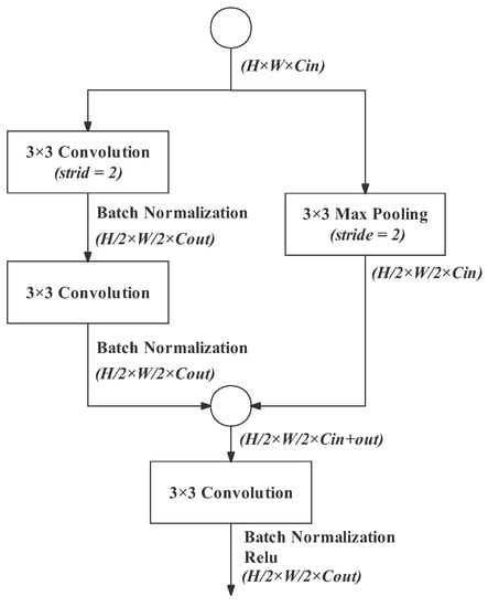
Figure 3.
Stem block. Notation: “3 × 3” in operation blocks denotes the operation’s kernel size; stride denotes the times of downsampling; the (H × W × C) label beneath each operation refers to the size of the output feature map (image); H: height, W:width, C: channel, while Cin denotes input channel and Cout denotes output channel.
The stem block plays the role of fast downsampling with a rate of 2 in both the detail path and the semantic branch. In the detail path, the stem block performs at the beginning of each stage. In the semantic branch, the first two stages are two successive stem blocks. The design of the stem block makes the dimensional expansion very flexible. It can expand the image to arbitrary suitable dimensions to meet different requirements. The detail path maintains spatial information with wide channels; therefore, the stem block in its first stage expands the channels from 3 to 32. The semantic branch needs narrow channels to reduce computational workload; therefore, the stem block in its first stage expands the channels slightly from 3 to 8. In other cases, the stem block doubles the number of channels.
3.3. Semantic Path
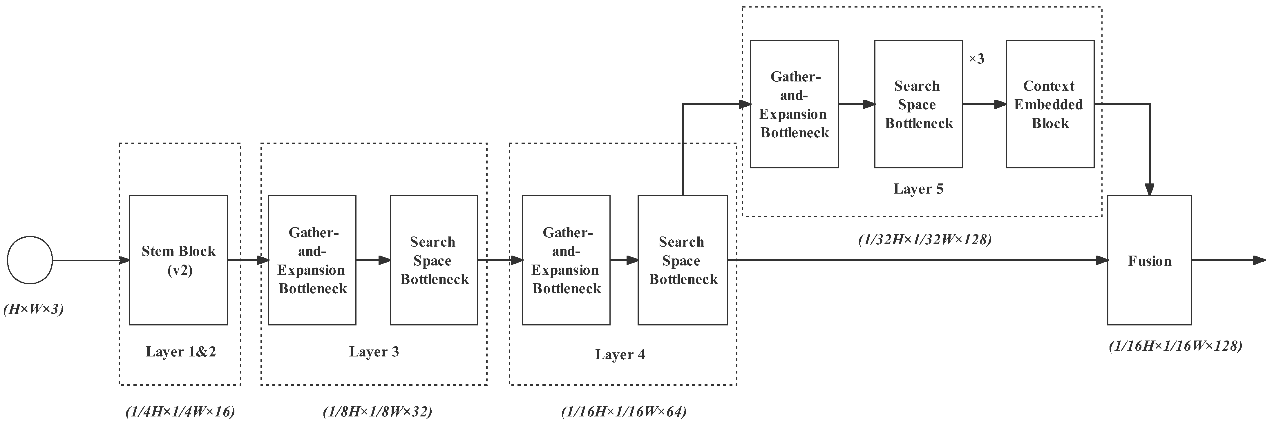
The semantic path is responsible for capturing semantic features of low resolution. We use deep structure and shallow channels to extract contextual feature representation. Since real-time detection requires the model to predict with low latency, we designed a lightweight network, shown in Figure 4.

- Layer 1 is a stem block we have introduced above. It shrinks the feature map size with a downsampling rate of 2 and enlarges the spatial slightly from 3 to 8 channels. With this layer, redundant information can be removed before complex computations;
- Layer 2 is as same as Layer 1, but it expands the channels from 8 to 16. The downsampling rate is 4;
- Gather–expand–search (GES) layers: Layers 3, 4, and 5, as well as the feature fusion layer constitute the GES layer. It mainly consists of a gather-and-expansion bottleneck and search-space bottlenecks. The gather-and-expansion bottleneck gathers feature representation by downsampling and storing spatial information by expanding channels. In each GES layer, a gather-and-expansion bottleneck is followed by several search-space bottlenecks. The search-space bottlenecks do not shrink the image size. They search for multi-resolution feature representations and integrate them. Detailed information for Layers 3, 4, 5 and the feature fusion layer is as follows:
- Layer 3: gather-and-expansion bottleneck + search-space bottleneck. The image channel is expanded to 32 and the downsampling rate is 8;
- Layer 4: The structure of Layer 4 is as same as Layer 2. Its output channel is 64 and the downsampling rate is 16;
- Layer 5: gather-and-expansion bottleneck + three search-space bottlenecks. In this layer, the output channel is 128, and the downsampling rate is 32. In the case of a high downsampling rate, plenty of search-space operations are particularly needed for enlarging the receptive field effectively. It can also further extract feature representation while maintaining the feature map size. In Layer 5, we also add the context-embedding block at the end to embed the global contextual information;
- The feature fusion layer is used for progressively aggregating the output feature of Layer 4 (downsampling rate of 16) and Layer 5 (downsampling rate of 32).
3.3.1. Gather–Expand–Search (GES) Layers with a Larger Receptive Field
The gather–expand–search (GES) layer is mainly composed of two kinds of bottlenecks: gather-and-expansion (GE) bottlenecks, which adopt depth-wise convolution and depth-wise separable convolution, and search-space bottlenecks, which adopt zoomed convolution. In addition, the GES layer also contains a context-embedding block and a feature fusion block.
Gather-and-Expansion Bottleneck
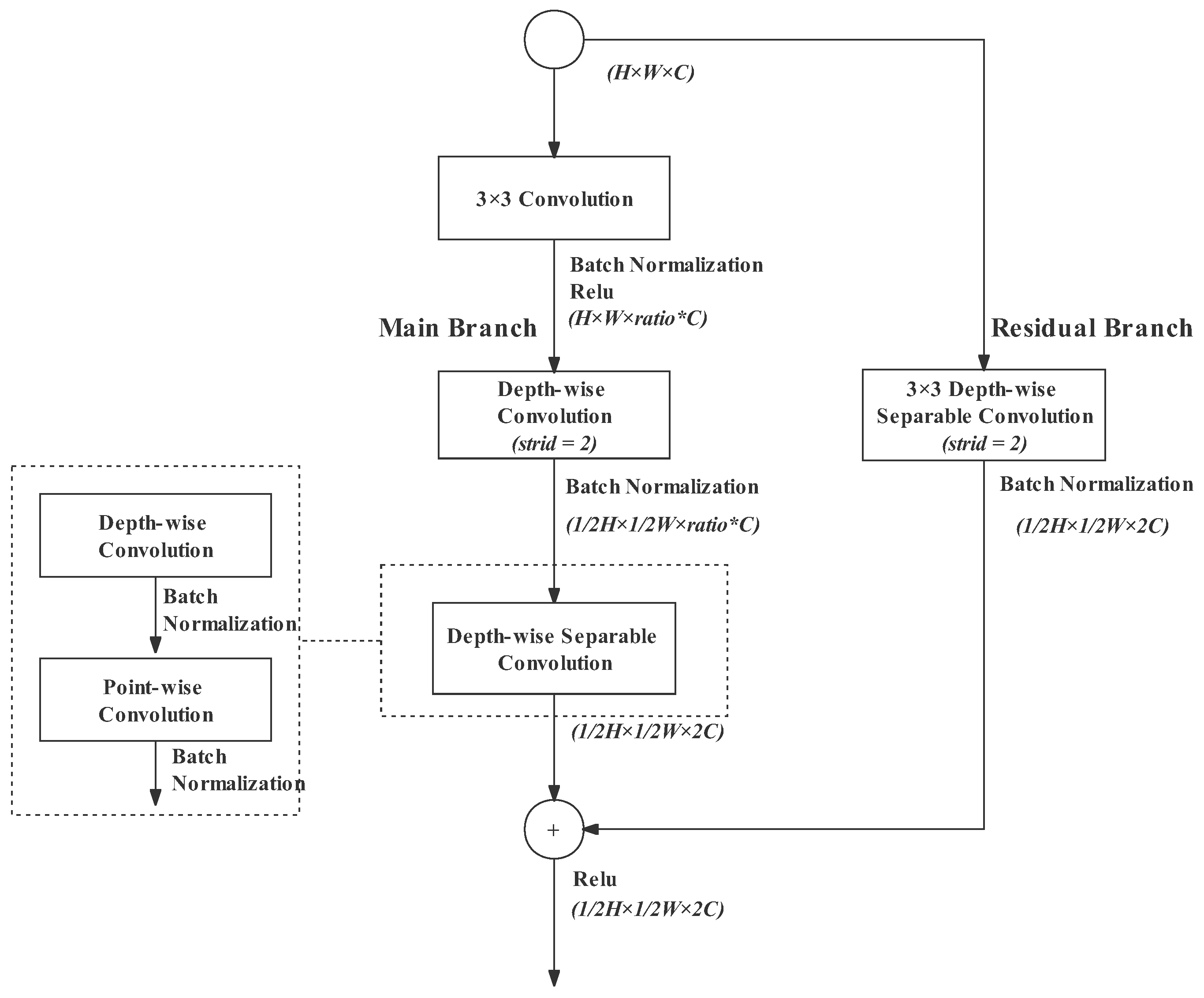
The gather-and-expansion (GE) bottleneck was proposed in MobileNetv2 and refined in BiSeNetv2 [30]. We adopt the design in BeSeNetv2 with improvements. The GE bottleneck aims to downsample the image to shrink the image size by half and double the dimension. The number of channels does not double directly. It is expanded with a relatively large ratio at first and projected to the desired dimension at the end. Such a design enables downsampling operations to deal with wide-channel feature maps; thus, abundant spatial information can be captured. As shown in Figure 5, the GE bottleneck consists of two branches: a main branch and a residual branch. The effect of each operation in the bottleneck is explained as follows:
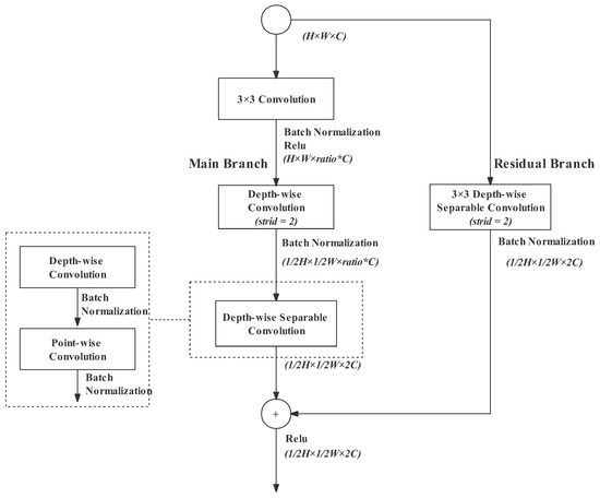
Figure 5.
Gather-and-expansion bottleneck. Notation: the dotted area on the left explains the structure of the depth-wise separable convolution in the main branch. The ratio is 6 in practice.
- 3 × 3 standard convolution: The 3 × 3 standard convolution with a stride of 1 at the beginning plays the role of channel expansion. The channels can be expanded with arbitrary appropriate ratios, but the experimental results in the BiSeNetv2 paper proved that the ratio of 6 has the best performance. Therefore, we also retained the ratio of 6 in our design;
- Depth-wise convolution: Depth-wise convolution performs a 3 × 3 convolution for each channel, reducing computational complexity significantly. In the original design in BiSeNetv2, the depth-wise convolution is responsible for channel expansion. However, in our design, the depth-wise convolution at any position does not change the number of channels. Our experimental results (in Section 3) proved that it will make the feature representation more accurate. In the main branch, the depth-wises convolution has a stride of 2, downsampling the feature map to half of the input;
- Depth-wise separable convolution: This is composed of a depth-wise convolution followed by a point-wise convolution. The depth-wise convolution conducts convolution on each channel separably and then the individual channels are combined by a point-wise convolution. The point-wise convolution is a 1 × 1 convolution. The 1 × 1 convolution is flexible for changing dimensions; therefore, it is also used to project the feature map into a narrower space of twice the input channels. In the main branch, the depth-wise separable convolution does not shrink image size;
- Residual branch: The residual branch can restore the input information and protect the neural network from degradation [33]. In order to fuse with the main branch, the residual branch needs the same downsampling rate as the main branch. Therefore, a depth-wise separable convolution with a stride of 2 is performed in the residual branch. The downsampling operation is performed in the depth-wise convolution.
At the end of the GE bottleneck, two feature maps are added together. Moreover, since the continuous activation function undermines the feature representation, a ReLU activation function is performed only when the output feature map is concatenated. In summary, the GE bottleneck extracts feature representation and shrinks the feature size with fast speed.
Search-Space Bottleneck
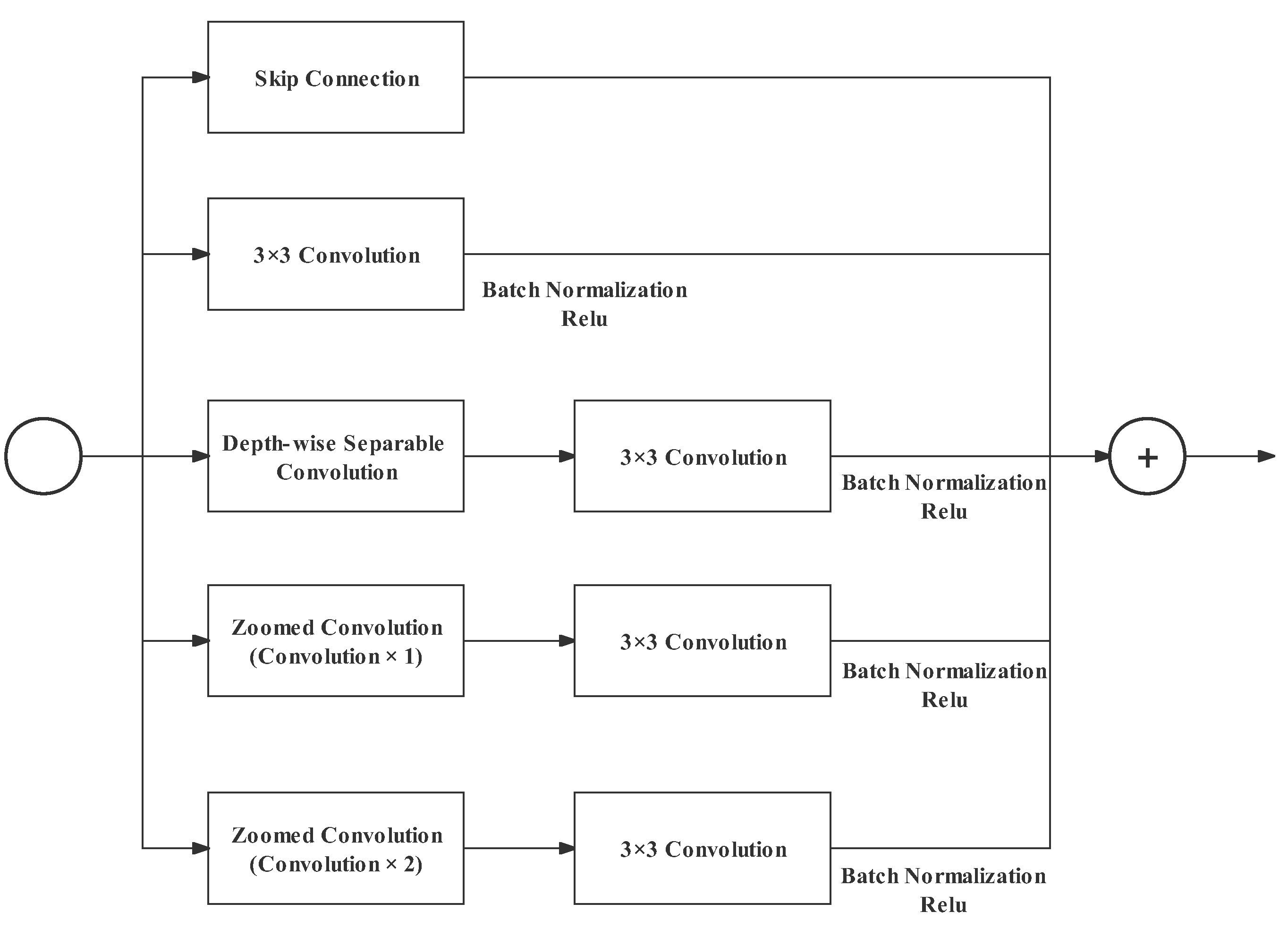
The search-space bottleneck aims to improve the accuracy of the result feature map of stages in the semantic path by enlarging the receptive field. The search-space bottleneck was first introduced in Auto-DeepLab [34] to optimize resolutions, and FasterSeg [32] designed the zoomed convolution for the search space. Zoomed convolution reduces 40% of the latency and doubles the receptive field [32] for a standard convolution. As shown in Figure 6, a zoomed convolution consists of one bilinear downsampling, one or more 3 × 3 convolutions, and a bilinear upsampling in sequence. Our design uses multiple parallel branches in the search-space bottleneck to integrate multi-resolution information. This design enables the search-space bottleneck to search for abundant information within the space and output a strong feature representation. In the search-space bottleneck, the size and the number of channels is kept stable. As shown in Figure 7, the parallel branches include:

Figure 6.
Zoomed convolution with two convolutions in the middle.
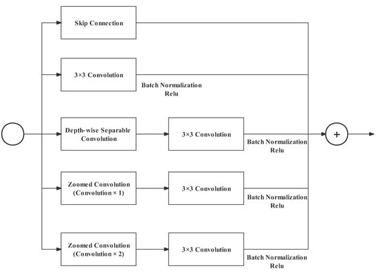
Figure 7.
Search-space bottleneck.
- Skip Connection: with this residual branch, more information can be utilized by subsequent blocks;
- A standard 3 × 3 convolution (with batch normalization and ReLU;.
- A depth-wise separable convolution followed by a standard 3 × 3 convolution. The structure of the depth-wise separable convolution is explained in the gather-and-expansion bottleneck;
- A zoomed convolution followed by a standard 3 × 3 convolution. The zoomed convolution here has one convolution in the middle (shown in Figure 7);
- Similar to Branch 4, but the zoomed convolution here has two convolutions (shown in Figure 8).
 Figure 8. Zoomed convolution with one convolution in the middle.
The additional 3 × 3 standard convolution at the end of Branches 3, 4, and 5 is used to strengthen the feature representation without adding significant cost because the 3 × 3 convolution is specially optimized in the CUDNN library [10]. In summary, the search-space bottleneck improves the accuracy of feature representation by extending the receptive field (zoomed convolution) and integrating multi-resolution features (parallel branches). Meanwhile, the zoomed convolution improves speed by reducing the convolution parameters.
Context-Embedding Block
The context-embedding block aims to capture high-level contextual information. In the case of a downsampling rate of 32, as the image size is shrunk to a great extent, a large receptive field is particularly needed. Therefore, a context-embedding block is added in the end of Layer 5 of the Semantic Branch. The BiSeNetv2 has a highly effective context-embedding block. Therefore, we adopt it in our network without modification. As shown in Figure 9, the context-embedding block consists of a main branch and a residual branch. In the main branch, the global average pooling provides adequate global information. In the end, there is also a standard 3 × 3 convolution to strengthen the feature representation.
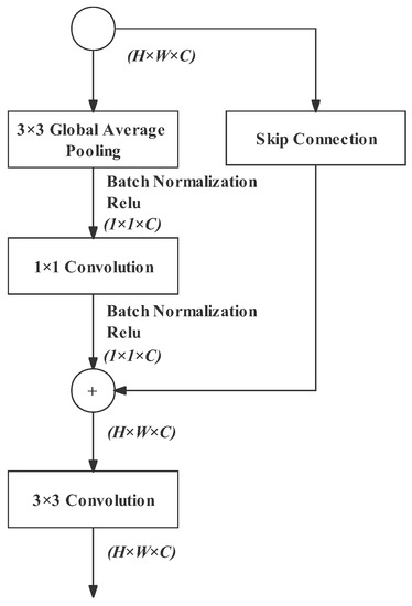
Figure 9.
Context-embedding block.
Feature Fusion
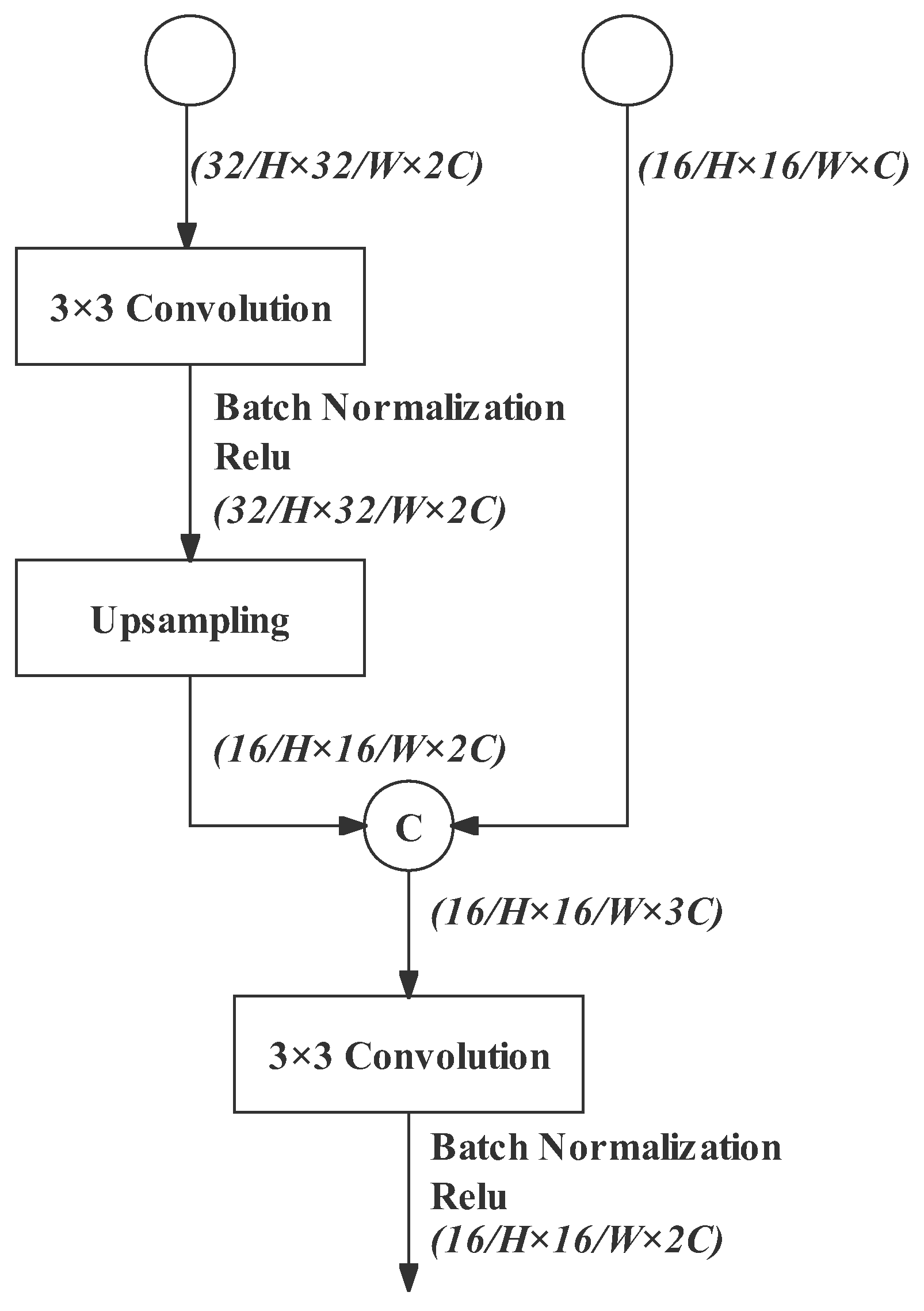
The output feature map of Layer 5 has a high-level feature representation with a downsampling rate of 32. However, its resolution is low level. The spatial information of its input feature map (the output of Layer 4) is inevitably damaged. This drawback can be solved by concatenating two outputs with different downsampling rates (32 for Layer 5 and 16 for Layer 4). As a result, the multi-resolution feature maps are integrated and the receptive field is enlarged.
The structure of the feature fusion block is shown in Figure 10. The feature map of Layer 5 output is further extracted by a standard 3 × 3 convolution and then upsampled. It is restored to 16 downsampling rate for fusing with Layer 4’s output. Since the channel amount of Layer 5’s output (128 channels) is also double that of Layer 4’s output (64 channels), the concatenated result (192 channels) is triple that of Layer 4’s output. Therefore, a standard 3 × 3 convolution projects the result into the desired dimension—128 channels, the same as the result of the detail path.
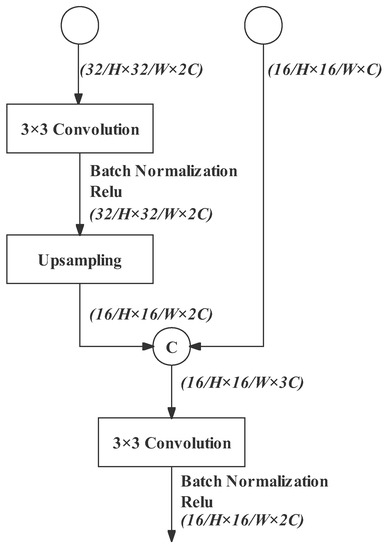
Figure 10.
Feature fusion block.
3.4. Detail Path
The detail path is responsible for low-level details with high resolution, adopting shallow layers and wide channels. The resulting feature map has a low downsampling rate of 8 and a wide channel number of 128. As shown in Figure 11, the detail path is composed of three stages. Each stage adopts a stem block for fast downsampling, shrinking the size to half and expanding channels. After the stem block, depth-wise separable convolutions are conducted to further extract feature representation with fast speed. There is also a standard convolution for feature strengthening in the last two stages.

Figure 11.
Detail path.
This design of the detail path ensures redundant information cleaning at the initial phase and then reserves information in spatial dimension (weight and height dimension). The convolution operation without ReLU can prevent the continuous activation function from damaging the feature accuracy. When the semantic path extracts feature representation but destroys spatial information, the detail path stores the spatial information. Later, these two kinds of information from two branches will integrate through the bilateral guided aggregation module.
3.5. Bilateral Guided Aggregation
This section is designed for fusing the output feature maps of the detail path and semantic path. As one is a low-level feature representation and the other is high-level, the two outputs cannot be merged by concatenation. In the bilateral guided aggregation of BiSeNetv2, the output of the detail path is downsampled and then merges with the semantic path. The contextual information from the semantic path guides the feature response during the downsampling. Meanwhile, the output of the semantic path also merges with the detail path after upsampling. This upsampling is guided by the spatial information from the detail path. This design enables the two branches to communicate efficiently.
In our design, we modified the structure of the bilateral guided aggregation of BiSeNetv2 to make it work more effectively. The output of the semantic branch in BiSeNetv2 is 1/32 of the original image size, while in our network, it is 1/16 of the original image size. Moreover, the channel width is the same in these two cases. Therefore, if we retain the feature-extraction operations in the bilateral guided aggregation of BiSeNetv2, too much computation and parameters will be added. Therefore, in our design, we need to simplify the bilateral guided aggregation block (shown in Figure 12). Note that the left branch deals with the output of the detail path, while the right branch deals with that of the semantic path.
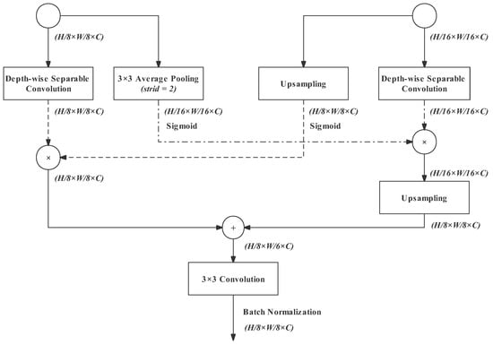
Figure 12.
Bilateral guided aggregation.
- Left Branch 1: A depth-wise separable convolution for further gathering feature representation fast;
- Left Branch 2: Average pooling with a stride of 2 results in a 16 downsampling rate. Its output will be fused with the output of the semantic path;
- Right Branch 1: The upsampling operation restores the output of the semantic path to an downsampling rate of 8. Its output will be fused with the output of detail path;
- Right Branch 2: Its structure and effect are as same as Left Branch 1.
Left Branch 1 and Right Branch 1 are multiplied together, and Right Branch 1 and Right Branch 2 are multiplied together. The result feature map of the Right Branch has a downsampling rate of 16. Therefore, it needs to be upsampled to a rate of 8. Thus, the output of the right branch and the left branch can be summed up together.
3.6. Segment Head with Training Boosting Strategy
3.6.1. Segment Head
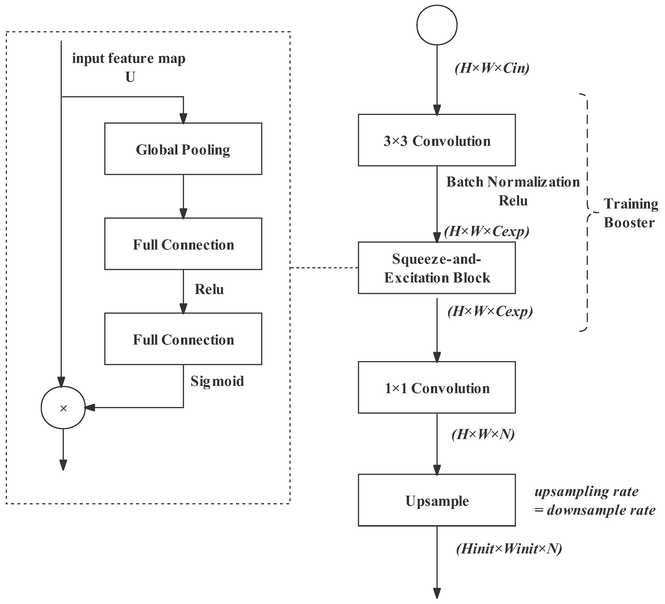
The segment head is located at the end of the network, where the input image is downsampled and expanded to high dimensions. Semantic segmentation is a pixel classification task. Therefore, to compute loss, the output size needs to be recovered to the initial size, and the number of channels should be equal to the number of label classes. This is completed by the last two operations in Figure 13. The 1 × 1 convolution projects the feature map to the N dimension space (N is the number of classes). Then, the feature map is upsampled to the initial size. The upsampling rate is equal to the downsampling rate of the feature map.
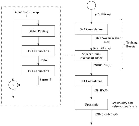
Figure 13.
Training boosting strategy.
In the BiSeNetv2, not only the final output of the network is involved in the loss computation, but also the partial outputs in the semantic path. We inherit this design, computing the loss for the partial output of Layers 2, 3, 4 and 5 in the semantic path, reinforcing the learning in the downsampling process. The final feature map is the output of bilateral guided aggregation (BGA). These loss values will be calculated individually and summed. The upsampling rates for Layer 2, Layer 3, Layer 4, Layer 5 and BGA are 4, 8, 16, 32, and 8, respectively.
3.6.2. Training Boosting Strategy
In the segment head, before the 1 × 1 convolution and upsampling, we also designed a training booster block to improve the quality of feature representation. The training boosting strategy increases the computation burden slightly in the training phase, but it can be totally discarded during inference. Therefore, the extra cost of the segment head does not need to be addressed.
The training booster block consists of a 3 × 3 convolution and a squeeze-and-excitation (SE) block. The 3 × 3 convolution expands the channels of the feature work to extract abundant spatial information. Then, the feature representation is further enhanced by the squeeze-and-excitation (SE) operation [35]. It can achieve feature recalibration, using global information to emphasize representative features while suppressing weak ones. The input feature map U first passes a squeeze operation. This is achieved by global average pooling. Through the squeeze operation, the spatial dimension features are aggregated. Then, an excitation operation fully extracts channel-wise dependencies. This is achieved by full connection (FC) followed by an activate function. There are two excitation operations: one uses ReLU as the activation function, while the other uses Sigmoid. The output is called scalar, and it then performs channel-wise multiplication with the input U.
4. Experimental Results
To evaluate the effectiveness of RecepNet, we trained and evaluated it with the benchmark dataset. In this section, we first introduce Cityscapes, the benchmark dataset we used. Then, we describe the training details. Third, we evaluate the effectiveness of each component of the network on the same dataset. Alternative plans for the design of the components will also be introduced and compared. The origin of the bilateral architecture is BiSeNetv2. Therefore, we compared the performance of each component and the overall network of our algorithm with BiSeNetv2.
4.1. Benchmark Dataset
Cityscapes [36] is a classical, challenging semantic segmentation dataset that focuses on urban street scenes from a car’s perspective. This dataset is split into three parts: 2975 for training, 500 for validation and 1525 for testing. In the experiments, we used finely annotated images in the Cityscapes dataset, which include 19 classes for semantic segmentation. Considering its high resolution of 2048 × 1024 pixels, these images are challenging for real-time semantic segmentation.
4.2. Training Details
4.2.1. General Training Settings
We trained our network from scratch. We adopted the stochastic gradient descent (SGD) as the optimizer and set the its parameters as weight decay = 5 × 10 and momentum = 0.9. Referring to BeSiNetv2, we adopted a “poly” learning rate strategy [10]. The initial learning rate was 5 × 10 and it was multiplied by for each iteration with the power of 0.9. denotes the current number of iterations. denotes the total number of iterations, which we set as 150K. Additionally, we chose 16 as the batch size.
4.2.2. Cost Function
As for the cost function, we used OhemCELoss (online hard example mining cross-entropy loss).
4.2.3. Image Augmentation
We also performed augmentation on the image data as follows:
- Randomly scale the image size. The scale value ranged from 0.25 to 2.0;
- Randomly horizontally flip the images;
- Randomly change the color jitter. The brightness was 0.4, the contrast was 0.4 and the saturation was 0.4.
All images with an original resolution of 2048 × 1024 were cropped to 1024 × 512 for training. Through image augmentation, the robustness of the network was enhanced.
4.2.4. Inference Details
The images were cropped to 1024 × 512 before inference. Additionally, we adopted image augmentation during the inference to improve the performance, including scaling the image size (from 0.25 to 2.0) and horizontally flipping the images. As for the evaluation metrics, we used the mean intersection over union (% mIoU)—the mean IoU value of all dataset classes. IoU is a standard performance metric for segmentation problems that measures the similarity between the predicted region and the ground-truth region in labels [37]. A higher % mIoU indicates a higher accuracy. Since image augmentation was conducted, the evaluation contained multi-scale crop evaluation and flip evaluation, which improved the accuracy to some extent.
We used GMACs (giga multiply–accumulate operations) to measure the computational cost of the model. The MAC (multiply–accumulate) operation, which is the basic operation in neural networks, calculates the product of two numbers and adds the result to an accumulator. We obtained the MAC count of the network by calculating and adding up the number of MACs in each convolutional layer. A smaller GMACs number indicates lower computational complexity [38].
4.3. Hardware Support
We built the implementation on PyTorch [39], an open-source machine learning framework for computer vision and language processing developed by Facebook. We trained the models using one NVIDIA RTX 3090 with CUDA 11. Moreover, we use FP16 precision for faster computation.
4.4. Component Evaluation
We used an ablation experiment to validate the effectiveness of each component of our algorithm, including the semantic path, detail path, bilateral guided aggregation layer and semantic head. We also compared the performance of the network components with those in BiSeNetv2, since BiSeNetV2 is the origin of the bilateral architecture and consists of these four components. In the ablation experiment, each individual test network assembled from blocks was retrained and fine-tuned on the Cityscapes dataset until it reached optimal performance. Thus, we proved that we make improvements to the overall network and its components.
4.4.1. Semantic Path
Design of Gather-and-Expansion Bottleneck
We referred to the inverted bottleneck (stride = 2) of BiSeNetv2 and improve its structure. To validate our improvement, we ran the semantic path of BiSeNetv2, but substituted all inverted bottlenecks (stride = 2) with our gather-and-expansion (GE) bottleneck. The result in Table 3 shows that our gather-and-expansion bottleneck improved the accuracy from 65.11% to 65.27%. This is because we used a convolution operation to expand the image to wide channels before downsampling, which can enlarge the spatial semantic field. Moreover, the depth-wise separable convolution can keep the number of parameters relatively small.

Table 3.
Performance of gather-and expansion bottleneck.
Design of Search-Space Bottleneck
To evaluate our design of the search-space bottleneck, we used the network in Figure 14. Here, for Layers 1 and 2, we still used the stem block in BiSeNetv2 (the stem block will be evaluated later).

Figure 14.
Network for search-space bottleneck testing.
The structure of Layers 3, 4 and 5 is the design in RecepNet. The search-space bottleneck in Layer 5 repeats three times. We adopt the context-embedding block in BiSeNetv2. Note that the blocks that are not annotated with “v2” belong to RecepNet.
Firstly, we designed the zoomed convolution, which is used in the search-space bottleneck. It has a larger receptive field, lower latency and fewer parameters than a standard convolution operation. The zoomed convolution starts with downsampling and ends with upsampling, and features are extracted in the middle process. Therefore, we tried several feature-extraction operations, aiming for better accuracy and lower complexity. To test the performance of different zoomed convolutions, only a single zoomed convolution was used in the search-space bottleneck of the test network (Figure 14). The results are shown in Table 4.

Table 4.
Performance of zoomed convolution with different structures. Notation: conv denotes convolution; 3 × 3 and 1 × 1 denote kernel size.
Considering accuracy and complexity, the structure of a 3 × 3 convolution followed by a depth-wise separable convolution has the best performance. That is because, although the accuracy of a depth-wise separable convolution is not as good as that of a standard convolution, it significantly reduces the algorithm complexity.
Secondly, we designed five parallel branches for the search-space bottleneck. To test the effectiveness of each branch, we designed a series of ablation experiments for the five branches. In the experiments, we used the test network in Figure 14. We also compared the final results in the “Design of Gather-and-Expansion Bottleneck” section.
The results in Table 5 show that the search-space bottleneck increases the accuracy significantly and simultaneously reduces the complexity. The skip branch can preserve the contextual information and the four branches with different convolution operations search for multi-resolution features. The integration of different branches provides the output with abundant information.

Table 5.
Ablation experiments for the search-space bottleneck. Notation: Skip denotes skip connection; conv denotes convolution; SepConv denotes depth-wise separable convolution; 3 × 3 denotes kernel size.
Design of Feature Fusion
As discussed above, we integrated the outputs of Layer 4 and Layer 5 to obtain multi-resolution feature maps, enhancing the receptive ability for spatial information. The test network is shown in Figure 15. The search-space bottleneck adopts the structure with the best performance in the last section (five parallel branches). The results in Table 6 show that feature representation is optimized and complexity only increases slightly, and is still lower than the semantic branch in BiSeNetv2.
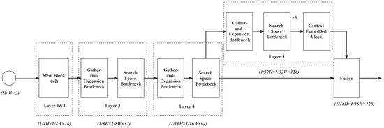
Figure 15.
Network for feature fusion testing.

Table 6.
Performance of feature fusion.
Fusion denotes feature fusion block. The output feature map of Layers 4 and 5 are fused through this feature fusion block.
4.4.2. Design of Stem Block
To test the design of our stem block, we replaced the BiSeNetv2 stem block in the last section’s test network (refer Figure 15) with our own design. It then became the complete semantic path of our RecepNet, shown previously in Figure 4. Table 7 shows that the new stem block improves accuracy while increasing some costs. This is because the combination of max pooling and two successive standard convolutions produce effective feature representation, while the repeated convolutions bring a small burden.

Table 7.
Performance of stem block.
Table 7 also indicates that, compared with the semantic path in BiSeNetv2, the semantic path in RecepNet makes impressive progress in both accuracy and speed.
4.4.3. Design of Detail Path
To illustrate the effectiveness of our detail path, we compare its performance with the original detail path in the BiSeNetv2. Table 8 shows that both the network simplicity and accuracy are considerably improved. The reason for this is that the stem block at the beginning of each stage completes fast downsampling, and the subsequent depth-wise separable convolutions enhance the feature representation with a slight cost.

Table 8.
Performance of detail path.
4.4.4. Design of Bilateral Guided Aggregation
Combining the output of the detail path and semantic path, we obtained a complete network of RecepNet without a training booster strategy. As shown in Table 9, RecepNet has a considerable advantage in accuracy. However, as discussed in Methodology, the output of the semantic path in the BiSeNetv2 is 1/32 of the original image size, while in RecepNet, it is 1/16 of the original image size. This will inevitably increase the computation in the bilateral guided aggregation because the image size is doubled with such a wide image channel (128). Luckily, since the complexity of the detail path and the semantic path in RecepNet is significantly lower than that in the BiSeNetv2 and our bilateral guided aggregation is simplified, the complexity of the whole network of RecepNet is just a little larger than that of BiSeNetv2.

Table 9.
Comparison of two networks without booster.
4.4.5. Design of Training Booster Strategy
Adding the training booster strategy, we can obtain a complete RecepNet. To validate the efficiency of our newly designed training booster strategy, we first used the training booster in BiSeNetv2 and, secondly, used our training booster. Then, we compared their performances. The result is shown in Table 10. Since the training booster strategy will be discarded in the inference phases, we do not increase complexity in Table 10 when applying the training booster strategy.

Table 10.
Performance of training booster strategy.
By observing the results, we can conclude that our training booster has better performance compared with the original one in BiSeNetv2. The reason for this is that the SE block plays a vital role in recalibrating the features.
4.4.6. Ablation Results Summary
In Table 11, we summarized all the’ performance of all components in RecepNet in the form of an ablation experiment. To be more convincing, we also compared the performance of each component with BiSeNetV2. Observing the results, we can see that, for each component, the accuracy of RecepNet is better than BiSeNetv2. In terms of complexity, the complexities of the detail path and the semantic path are lower than in BiSeNetv2. However, after adding the aggregation module, RecepNet has a higher computational complexity. This is because the output of the semantic path in BiSeNetV2 is downsampled by 1/32, while in RecepNet it is downsampled by 16. Therefore, the feature map with a large size and wide channels brings a computational burden. We designed a simple structure for the aggregation module to minimize the increase of complexity.

Table 11.
Component performance and overall performance of RecepNet.
In summary, RecepNet is superior to BiSeNetV2 because it improves the accuracy significantly (from 73 to 78) at a negligible cost of complexity (just 0.4 GMACs).
4.5. Inference Speed
We also tested the network’s inference speed on one RTX 3090 GPU. The inference speed is measured in frames per second (FPS), which means how many frames can be processed per second. Please note that FPS depends on GPU performance, while the % mIoU and GMACs are only related to the algorithm. Generally, an algorithm with lower GMACs has a higher FPS on the same machine. We chose Deeplabv3+ and BiSeNetV2 as the comparative networks. That is because the accuracy of DeepLabv3+ has been excellent in works of recent years and BiSeNetV2 has outstanding speed.
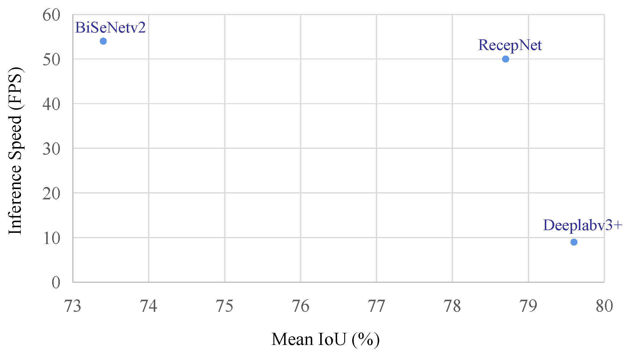
The speed and accuracy of the three networks are shown in Figure 16. Comparing the results, we can see that RecepNet has an accuracy approximating that of DeepLabV3+, and its inference speed approximates that of BiSeNetV2. Among the three networks, RecepNet has the longest projection on the diagonal of the chart. We can thus conclude that as a high-speed real-time semantic segmentation network, RecepNet also has competitive performance in accuracy.

Figure 16.
Comparison of three networks. Axis x denotes mIoU. A network placed higher in Axis x shows higher accuracy. Axis y denotes inference speed in FPS; A network placed higher in Axis y shows faster inference speed.
5. Application in Blue-Green Algae Detection
In recent years, advanced technologies such as soft-computing and machine learning have been widely used in environment prediction and management, including support vector regression, (SVR), relevance vector machine (RVM) and multiple recursive nesting bias correction (MRNBC) [40]. Other methods, including artificial neural network (ANN), adaptive neuro fuzzy inference system (ANFIS), M5P and random forest (RF), have also been implemented [41]. Statistical analysis methods, such as the first-order second-moment statistical method [42], have been used to predict the impact of aquatic organisms on aquatic ecosystems. An intellectual detection approach for blue-green algae is needed by water environment treatment industry. Blue-green algae smell musty and their blooms can produce toxins that are released into the water and lead to livestock deaths [43]. Especially for blue-green algae blooms in lakes and rivers providing drinking water, the polluted water can cause human diseases, such as diarrhea and hepatitis [43]. Currently, there are various prevalent methods for blue-green algae detection, such as analyzing the water sample using a PCR-DCG detecting kit [44]. Currently, the outbreak of blue-green algae can be detected with UAVs. The cameras embedded in UAVs take aerial images of the water surface; then, the blue-green algae is manually identified on the aerial images of the water surface. However, this method requires huge labor due to the vast area of natural waters. To solve this problem, we firstly propose to use UAV to real-time detect blue-green algae through an embedded computer vision system. It is achieved by making a blue-green algae dataset using those aerial images and then training our RecepNet on the dataset.
5.1. Blue-Green Algae Dataset
Our blue-green algae dataset is split into a training set and a validation set. The training set contains 1044 images and the validation set contains 261 images. The dataset link is available at Data Availability Statement part.
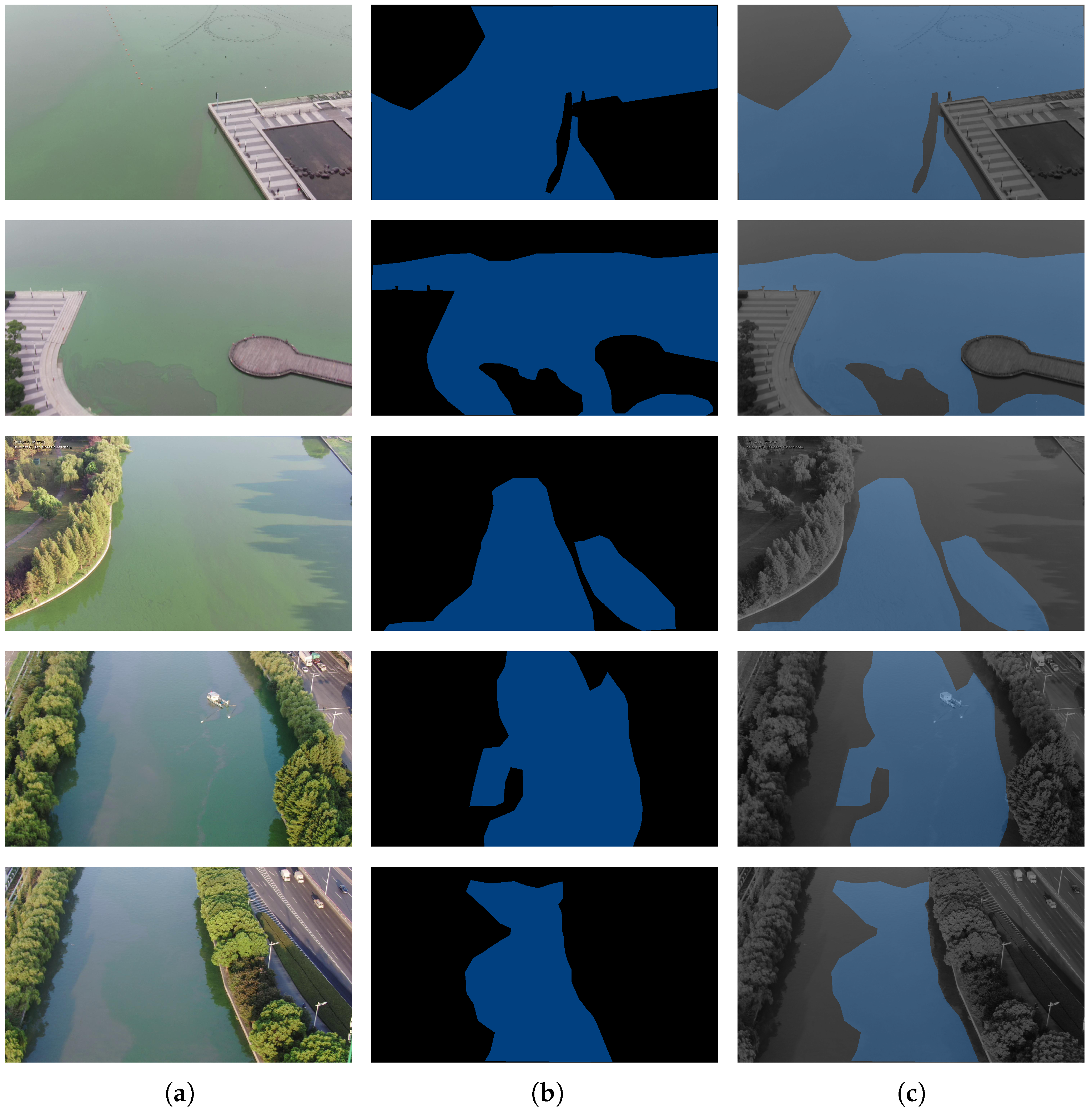
Raw images: The raw data are aerial images of rivers and lakes where blue-green algae appears. As blue-green algae grow on the water surface, aerial images can be used to detect its explosion efficiently. However, as the color of both water and blue-green algae is green, accuracy is challenging in this task. Examples of aerial images of blue-green algae are shown in Figure 17.
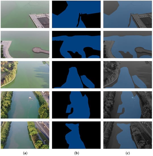
Figure 17.
Raw images and masks in dataset. The first column titled (a) are the original images taken by UAVs. The second column titled (b) are the labels, with the blue areas representing blue-green algae. The third column titled (c) are the fused images, in order to clearly present the results; (a), raw images; (b), masks; (c), blends.
Image annotation: The blue-green algae area in each image are labeled manually using LabelMe, a graphical annotation tool of Anaconda. A JSON file is generated for each image to store annotation information.
Formatting dataset: Before use, the mask for each image should be generated using the JSON files. We generate masks in the Cityscapes format, which uses single-channel grayscale labels. The grayscale value of the class (target) is n [36]. In this task, we just have a single target: algae. Such mask images cannot be recognized clearly. Therefore, to present our result, we convert the target area to a blue color and blend the mask image with a raw image (only for illustration). Figure 17 shows the raw images, masks, and masks blended with the raw images.
5.2. Network Performance on Blue-Green Algae Dataset
The training configuration is as same as with the Cityscapes dataset. After training with RecepNet, we tested the model inference performance on the validation set. Compared with the original BisenetV2, which had an accuracy of 79.51% mIoU on the algae validation set, our RecepNet achieved 82.12% mIoU, shown in Table 12. Figure 18 shows some examples of inference. RecepNet had an inference speed of 50.12 FPS on an RTX 3090, which is much higher than the 30 FPS of cameras, meaning it could easily process all 30 frames per second from a camera video stream. Thus, we conclude that our algorithm can process semantic segmentation in real time. Additionally, our blue-green algae dataset is effective.

Table 12.
Comparison of RecepNet, BiSeNetv2 and DeepLabv3+’s performance on blue-green algae detection.
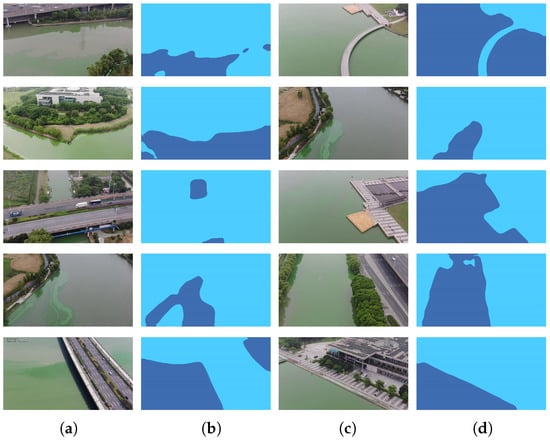
Figure 18.
Inference on blue-green algae dataset. The first and third columns titled (a) are the original images; the second and fourth columns titled (b) are labels, where the dark blue part is the identified blue-green algae area; (c), raw images; (d), inference results.
6. Conclusions
This paper proposed a novel real-time semantic segmentation network, RecepNet. Its detail path uses wide channel convolutional layers to extract and preserve high-resolution features. The lightweight network gather–expand–search (GES) in the semantic path searches and gathers rich semantic and spatial information. A bilateral aggregation model fuses the output of the two paths with a simple structure. Furthermore, a novel training booster strategy recalibrates and enhances features in the training phases. We proposed several blocks with low complexity to expand the network’s spatial and semantic receptive fields, including the stem block, the gather-and-expansion bottleneck and the search-space bottleneck. Experimental results show that the proposed RecepNet has good performance in both accuracy and speed on the Cityscapes dataset and blue-green algae dataset. In the future, we can calculate the area of the detected blue-green algae explosion utilizing the vision system and depth information.
Author Contributions
Conceptualization, K.Y.; methodology, K.Y.; software, K.Y. and Z.W.; validation, K.Y., Z.W., Z.Y. and P.Z.; formal analysis, Z.Y. and P.Z.; resources, S.Y.; writing—original draft preparation, K.Y.; writing—review and editing, K.Y. and X.Z.; supervision, X.Z., Y.Y., W.W., J.M. and J.Z. All authors have read and agreed to the published version of the manuscript.
Funding
This research was supported by the Suzhou Science and Technology Project (SYG202006, SYG202122), the Key Program Special Fund of Xi’an Jiaotong-Liverpool University (XJTLU) (KSF-A-19, KSF-E-65, KSF-P-02, KSF-E-54), the Research Development Fund of XJTLU (RDF-19-02-23), the National Natural Science Foundation of China (62002296) and the Natural Science Foundation of Jiangsu Province (BK20200250).
Data Availability Statement
The image dataset of blue-green algae semantic segmentation is available at https://www.kaggle.com/datasets/beyondstellaris/bluegreen-algae-dataset (accessed on 11 August 2022).
Acknowledgments
We thank Tianlei Shi for his valuable advice on the project and Xiangyu Sha for her contribution on the dataset annotation.
Conflicts of Interest
The authors declare no conflict of interest.
References
- Kang, Y.; Yamaguchi, K.; Naito, T.; Ninomiya, Y. Multiband Image Segmentation and Object Recognition for Understanding Road Scenes. IEEE Trans. Intell. Transp. Syst. 2011, 12, 1423–1433. [Google Scholar] [CrossRef]
- Chen, B.; Gong, C.; Yang, J. Importance-Aware Semantic Segmentation for Autonomous Vehicles. IEEE Trans. Intell. Transp. Syst. 2019, 20, 137–148. [Google Scholar] [CrossRef]
- Zeng, D.; Chen, X.; Zhu, M.; Goesele, M.; Kuijper, A. Background Subtraction With Real-Time Semantic Segmentation. IEEE Access 2019, 7, 153869–153884. [Google Scholar] [CrossRef]
- Simonyan, K.; Zisserman, A. Very deep convolutional networks for large-scale image recognition. arXiv 2014, arXiv:1409.1556. [Google Scholar]
- He, K.; Zhang, X.; Ren, S.; Sun, J. Deep residual learning for image recognition. In Proceedings of the IEEE Conference on Computer Vision and Pattern Recognition, Las Vegas, NV, USA, 27–30 June 2016; pp. 770–778. [Google Scholar]
- Chen, L.C.; Zhu, Y.; Papandreou, G.; Schroff, F.; Adam, H. Encoder-Decoder with Atrous Separable Convolution for Semantic Image Segmentation. arXiv 2018, arXiv:1802.02611. [Google Scholar]
- Paszke, A.; Chaurasia, A.; Kim, S.; Culurciello, E. ENet: A Deep Neural Network Architecture for Real-Time Semantic Segmentation. arXiv 2016, arXiv:1606.02147. [Google Scholar]
- Treml, M.; Arjona-Medina, J.; Unterthiner, T.; Durgesh, R.; Friedmann, F.; Schuberth, P.; Mayr, A.; Heusel, M.; Hofmarcher, M.; Widrich, M.; et al. Speeding up semantic segmentation for autonomous driving. In Proceedings of the MLITS, NIPS Workshop, Barcelona, Spain, 1 October 2016. [Google Scholar]
- Lin, G.; Milan, A.; Shen, C.; Reid, I. Refinenet: Multi-path Refinement Networks for High-Resolution Semantic Segmentation. In Proceedings of the IEEE Conference on Computer Vision and Pattern Recognition, Honolulu, HI, USA, 21–26 July 2017; pp. 1925–1934. [Google Scholar]
- Yu, C.; Gao, C.; Wang, J.; Yu, G.; Shen, C.; Sang, N. BiSeNet V2: Bilateral Network with Guided Aggregation for Real-time Semantic Segmentation. arXiv 2020, arXiv:2004.02147. [Google Scholar] [CrossRef]
- Otsu, N. A Threshold Selection Method from Gray-Level Histograms. IEEE Trans. Syst. Man Cybern. 1979, 9, 62–66. [Google Scholar] [CrossRef]
- Mottaghi, R.; Chen, X.; Liu, X.; Cho, N.G.; Lee, S.W.; Fidler, S.; Urtasun, R.; Yuille, A. The Role of Context for Object Detection and Semantic Segmentation in the Wild. In Proceedings of the IEEE Conference on Computer Vision and Pattern Recognition, Columbus, OH, USA, 23–28 June 2014; pp. 891–898. [Google Scholar]
- Shotton, J.; Winn, J.; Rother, C.; Criminisi, A. Textonboost for Image Understanding: Multi-class Object Recognition and Segmentation by Jointly Modeling Texture, Layout, and Context. Int. J. Comput. Vis. 2009, 81, 2–23. [Google Scholar] [CrossRef]
- Achanta, R.; Shaji, A.; Smith, K.; Lucchi, A.; Fua, P.; Süsstrunk, S. SLIC Superpixels Compared to State-of-the-Art Superpixel Methods. IEEE Trans. Pattern Anal. Mach. Intell. 2012, 34, 2274–2282. [Google Scholar] [CrossRef]
- Kalchbrenner, N.; Grefenstette, E.; Blunsom, P. A Convolutional Neural Network for Modelling Sentences. In Proceedings of the 52nd Annual Meeting of the Association for Computational Linguistics (Volume 1: Long Papers); Association for Computational Linguistics: Baltimore, MD, USA, 2014; pp. 655–665. [Google Scholar] [CrossRef]
- Long, J.; Shelhamer, E.; Darrell, T. Fully Convolutional Networks for Semantic Segmentation. arXiv 2015, arXiv:1411.4038. [Google Scholar]
- Chen, L.C.; Papandreou, G.; Kokkinos, I.; Murphy, K.; Yuille, A.L. Semantic Image Segmentation with Deep Convolutional Nets and Fully Connected CRFs. arXiv 2016, arXiv:1412.7062. [Google Scholar]
- Chen, L.C.; Papandreou, G.; Kokkinos, I.; Murphy, K.; Yuille, A.L. Deeplab: Semantic Image Segmentation with Deep Convolutional Nets, Atrous Convolution, and Fully Connected Crfs. IEEE Trans. Pattern Anal. Mach. Intell. 2017, 40, 834–848. [Google Scholar] [CrossRef] [PubMed]
- Zhao, H.; Shi, J.; Qi, X.; Wang, X.; Jia, J. Pyramid Scene Parsing Network. arXiv 2017, arXiv:1612.01105. [Google Scholar]
- Yuan, Y.; Wang, J. Ocnet: Object Context Network for Scene Parsing. arXiv 2018, arXiv:1809.00916. [Google Scholar]
- Zhao, H.; Zhang, Y.; Liu, S.; Shi, J.; Loy, C.C.; Lin, D.; Jia, J. Psanet: Point-wise Spatial Attention Network for Scene Parsing. In Proceedings of the European Conference on Computer Vision (ECCV), Munich, Germany, 8–14 September 2018; pp. 267–283. [Google Scholar]
- Ronneberger, O.; Fischer, P.; Brox, T. U-Net: Convolutional Networks for Biomedical Image Segmentation. In Proceedings of the International Conference on Medical Image Computing and Computer-Assisted Intervention, Munich, Germany, 5–9 October 2015; Springer: Berlin/Heidelberg, Germany, 2015; pp. 234–241. [Google Scholar]
- Yu, C.; Wang, J.; Peng, C.; Gao, C.; Yu, G.; Sang, N. Learning a Discriminative Feature Network for Semantic Segmentation. In Proceedings of the IEEE Conference on Computer Vision and Pattern Recognition, Salt Lake City, UT, USA, 23–28 June 2018; pp. 1857–1866. [Google Scholar]
- Wang, J.; Sun, K.; Cheng, T.; Jiang, B.; Deng, C.; Zhao, Y.; Liu, D.; Mu, Y.; Tan, M.; Wang, X.; et al. Deep High-Resolution Representation Learning for Visual Recognition. IEEE Trans. Pattern Anal. Mach. Intell. 2020, 43, 3349–3364. [Google Scholar] [CrossRef]
- Zheng, S.; Jayasumana, S.; Romera-Paredes, B.; Vineet, V.; Su, Z.; Du, D.; Huang, C.; Torr, P.H. Conditional Random Fields as Recurrent Neural Networks. In Proceedings of the IEEE International Conference on Computer Vision, Washington, DC, USA, 7–13 December 2015; pp. 1529–1537. [Google Scholar]
- Mehta, S.; Rastegari, M.; Caspi, A.; Shapiro, L.; Hajishirzi, H. Espnet: Efficient Spatial Pyramid of Dilated Convolutions for Semantic Segmentation. In Proceedings of the European Conference on Computer Vision (ECCV), Munich, Germany, 8–14 September 2018; pp. 552–568. [Google Scholar]
- Romera, E.; Alvarez, J.M.; Bergasa, L.M.; Arroyo, R. Erfnet: Efficient Residual Factorized Convnet for Real-Time Semantic Segmentation. IEEE Trans. Intell. Transp. Syst. 2017, 19, 263–272. [Google Scholar] [CrossRef]
- Zhao, H.; Qi, X.; Shen, X.; Shi, J.; Jia, J. Icnet for Real-Time Semantic Segmentation on High-Resolution Images. In Proceedings of the European Conference on Computer Vision (ECCV), Munich, Germany, 8–14 September 2018; pp. 405–420. [Google Scholar]
- Wang, Y.; Zhou, Q.; Liu, J.; Xiong, J.; Gao, G.; Wu, X.; Latecki, L.J. Lednet: A Lightweight Encoder-Decoder Network for Real-Time Semantic Segmentation. In Proceedings of the 2019 IEEE International Conference on Image Processing (ICIP), Taipei, Taiwan, 22–25 September 2019; pp. 1860–1864. [Google Scholar]
- Sandler, M.; Howard, A.; Zhu, M.; Zhmoginov, A.; Chen, L.C. MobileNetV2: Inverted Residuals and Linear Bottlenecks. arXiv 2019, arXiv:1801.04381. [Google Scholar]
- Zhang, X.; Zhou, X.; Lin, M.; Sun, J. Shufflenet: An Extremely Efficient Convolutional Neural Network for Mobile Devices. In Proceedings of the IEEE Conference on Computer Vision and Pattern Recognition, Salt Lake City, UT, USA, 18–22 June 2018; pp. 6848–6856. [Google Scholar]
- Chen, W.; Gong, X.; Liu, X.; Zhang, Q.; Li, Y.; Wang, Z. FasterSeg: Searching for Faster Real-time Semantic Segmentation. arXiv 2020, arXiv:1912.10917. [Google Scholar]
- Wu, D.; Wang, Y.; Xia, S.T.; Bailey, J.; Ma, X. Skip Connections Matter: On the Transferability of Adversarial Examples Generated with Resnets. arXiv 2020, arXiv:2002.05990. [Google Scholar]
- Liu, C.; Chen, L.C.; Schroff, F.; Adam, H.; Hua, W.; Yuille, A.; Li, F.-F. Auto-DeepLab: Hierarchical Neural Architecture Search for Semantic Image Segmentation. arXiv 2019, arXiv:1901.02985. [Google Scholar]
- Hu, J.; Shen, L.; Albanie, S.; Sun, G.; Wu, E. Squeeze-and-Excitation Networks. arXiv 2019, arXiv:1709.01507. [Google Scholar]
- Cordts, M.; Omran, M.; Ramos, S.; Rehfeld, T.; Enzweiler, M.; Benenson, R.; Franke, U.; Roth, S.; Schiele, B. The Cityscapes Dataset for Semantic Urban Scene Understanding. In Proceedings of the IEEE Conference on Computer Vision and Pattern Recognition, Las Vegas, NV, USA, 26 June–1 July 2016; pp. 3213–3223. [Google Scholar]
- Rahman, M.A.; Wang, Y. Optimizing intersection-over-union in deep neural networks for image segmentation. In Proceedings of the International Symposium on Visual Computing, Las Vegas, NV, USA, 12–14 December 2016; Springer: Berlin/Heidelberg, Germany, 2016; pp. 234–244. [Google Scholar]
- Biswas, A.; Chandrakasan, A.P. CONV-SRAM: An energy-efficient SRAM with in-memory dot-product computation for low-power convolutional neural networks. IEEE J. Solid-State Circuits 2018, 54, 217–230. [Google Scholar] [CrossRef]
- Paszke, A.; Gross, S.; Massa, F.; Lerer, A.; Bradbury, J.; Chanan, G.; Killeen, T.; Lin, Z.; Gimelshein, N.; Antiga, L.; et al. Pytorch: An Imperative Style, High-Performance Deep Learning Library. Adv. Neural Inf. Process. Syst. 2019, 32, 8026–8037. [Google Scholar]
- Sarhadi, A.; Burn, D.H.; Johnson, F.; Mehrotra, R.; Sharma, A. Water resources climate change projections using supervised nonlinear and multivariate soft computing techniques. J. Hydrol. 2016, 536, 119–132. [Google Scholar] [CrossRef]
- Sadeghifar, T.; Lama, G.; Sihag, P.; Bayram, A.; Kisi, O. Wave height predictions in complex sea flows through soft-computing models: Case study of Persian Gulf. Ocean. Eng. 2022, 245, 110467. [Google Scholar] [CrossRef]
- Lama, G.; Errico, A.; Pasquino, V.; Mirzaei, S.; Preti, F.; Chirico, G. Velocity Uncertainty Quantification based on Riparian Vegetation Indices in open channels colonized by Phragmites australis. J. Ecohydraulics 2022, 7, 71–76. [Google Scholar] [CrossRef]
- Vu, H.P.; Nguyen, L.N.; Zdarta, J.; Nga, T.T.; Nghiem, L.D. Blue-Green Algae in Surface Water: Problems and Opportunities. Curr. Pollut. Rep. 2020, 6, 105–122. [Google Scholar] [CrossRef]
- Hu, Z.; Luo, W. Method for Detecting Water Body Blue Algae Based on PCR-DCG and Kit Thereof. China Patent CN101701264B, 28 December 2011. [Google Scholar]
Publisher’s Note: MDPI stays neutral with regard to jurisdictional claims in published maps and institutional affiliations. |
© 2022 by the authors. Licensee MDPI, Basel, Switzerland. This article is an open access article distributed under the terms and conditions of the Creative Commons Attribution (CC BY) license (https://creativecommons.org/licenses/by/4.0/).

