


Two-Dimensional InSAR Monitoring of the Co- and Post-Seismic Ground Deformation of the 2021 Mw 5.9 Arkalochori (Greece) Earthquake and Its Impact on the Deformations of the Heraklion City Wall Relic


 , ,
, , 
Abstract

1. Introduction
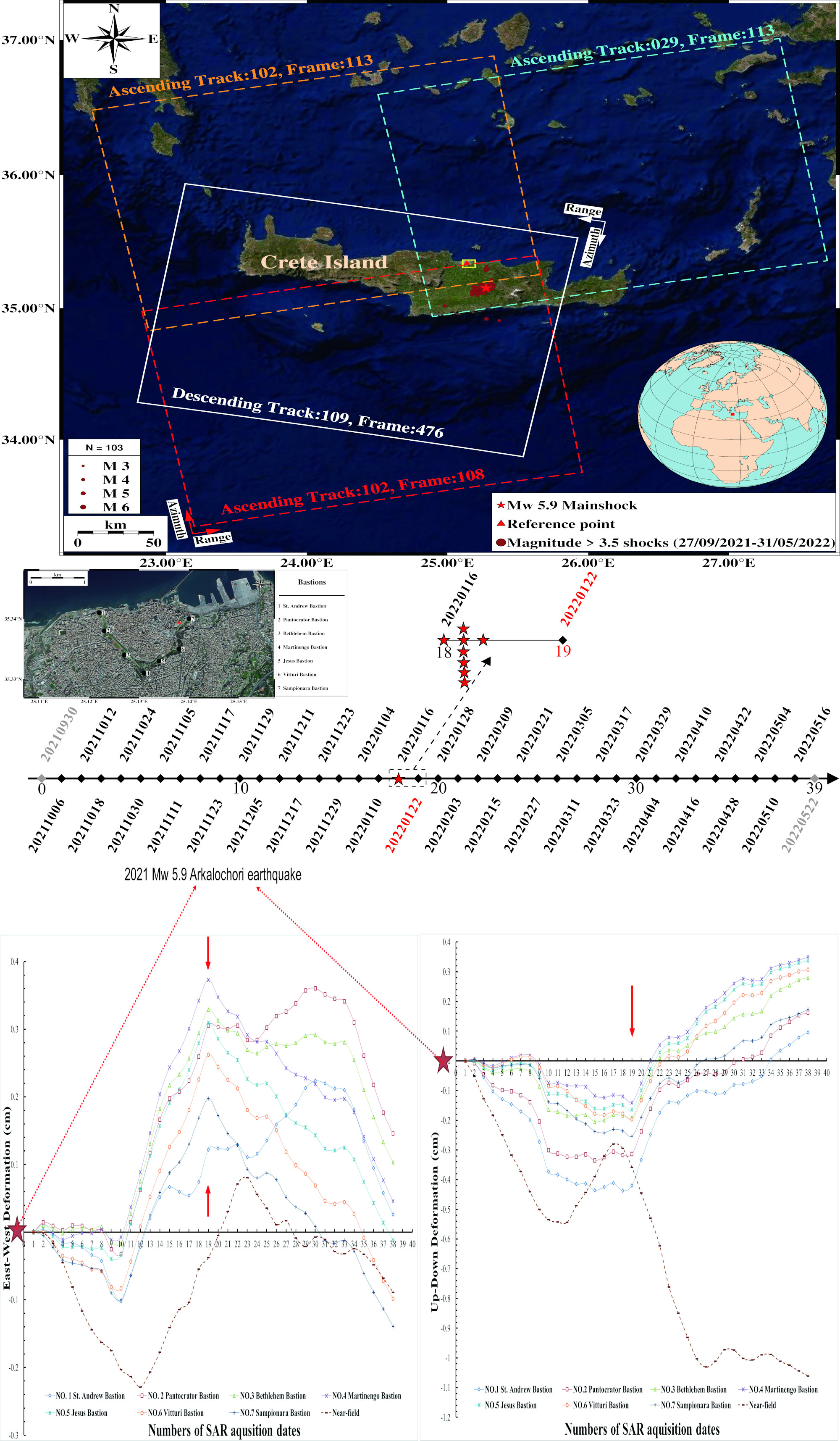
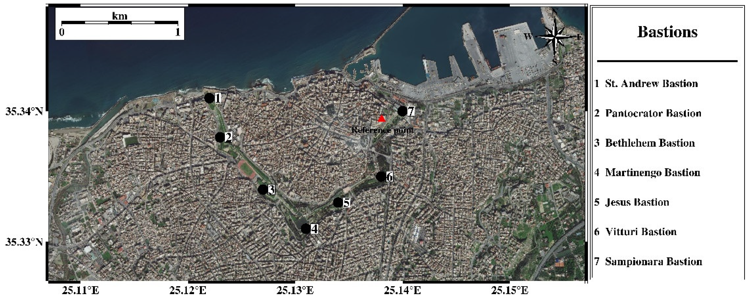
2. Study Area
3. Materials and Methods
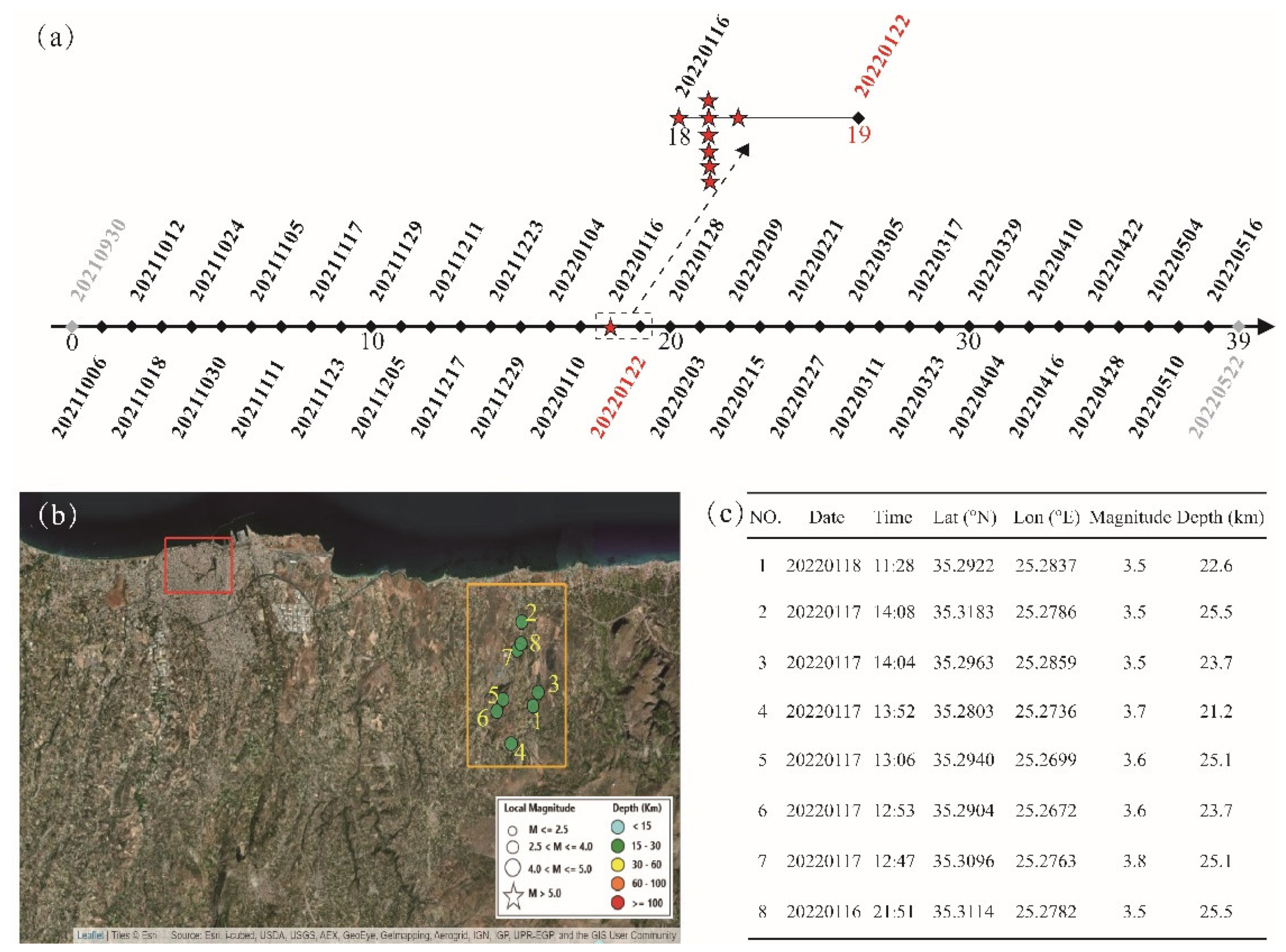
3.1. SAR Datasets
3.2. D-InSAR Processing
3.3. MSBAS Processing
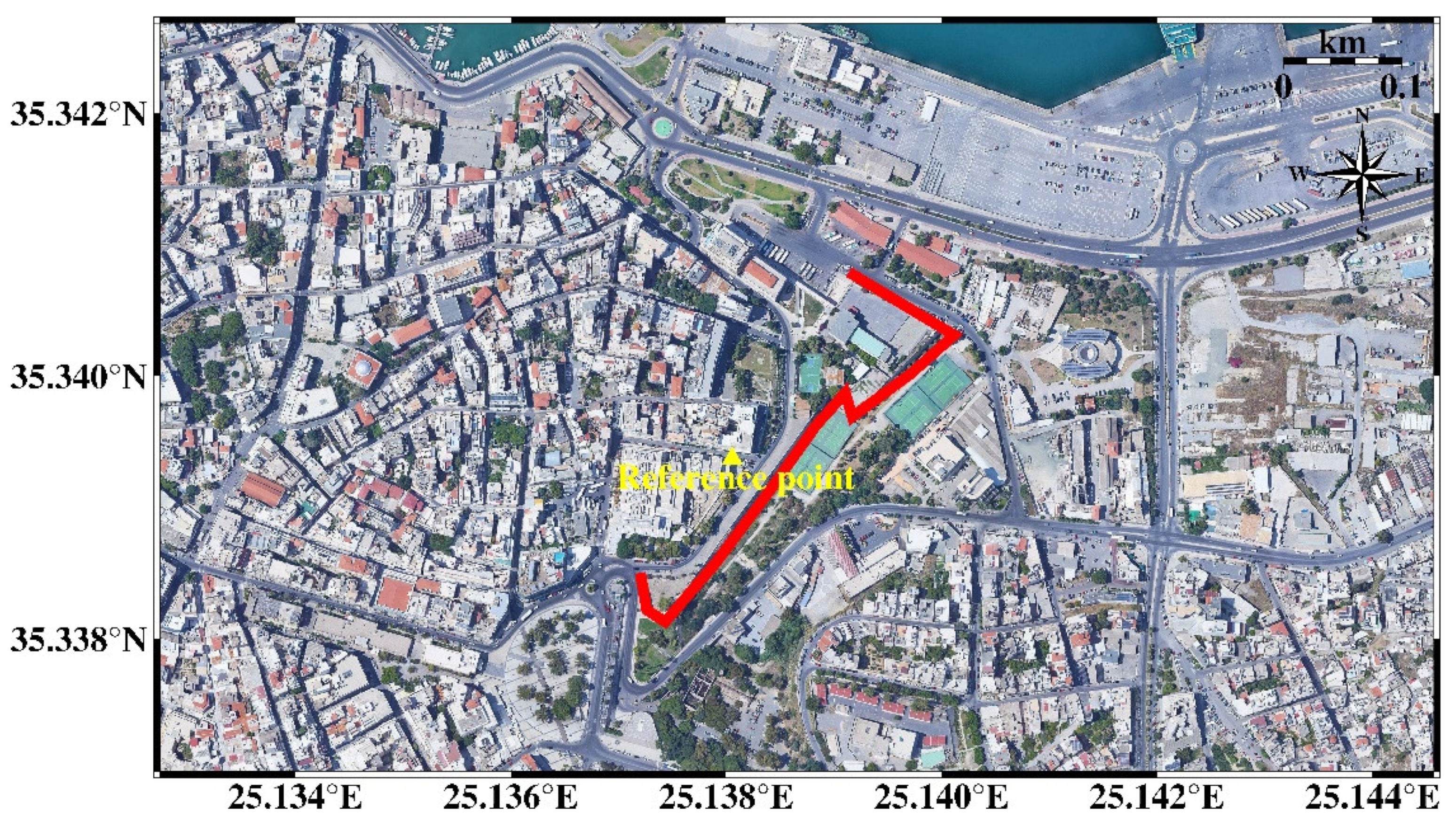
3.4. Reference Point Selecting
4. Results
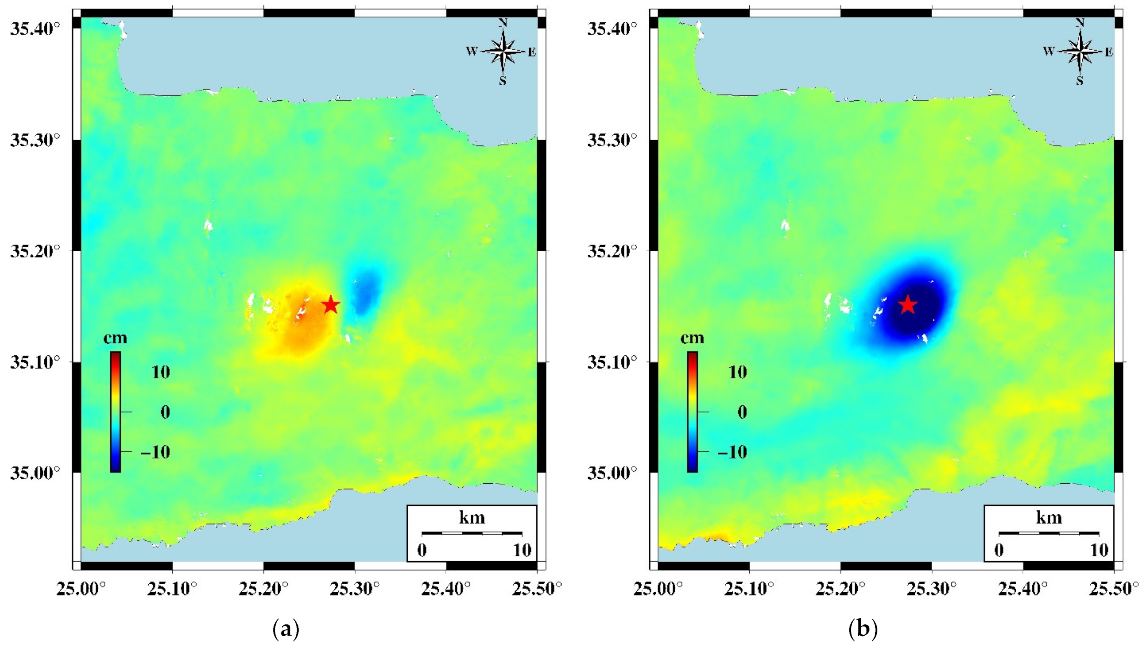
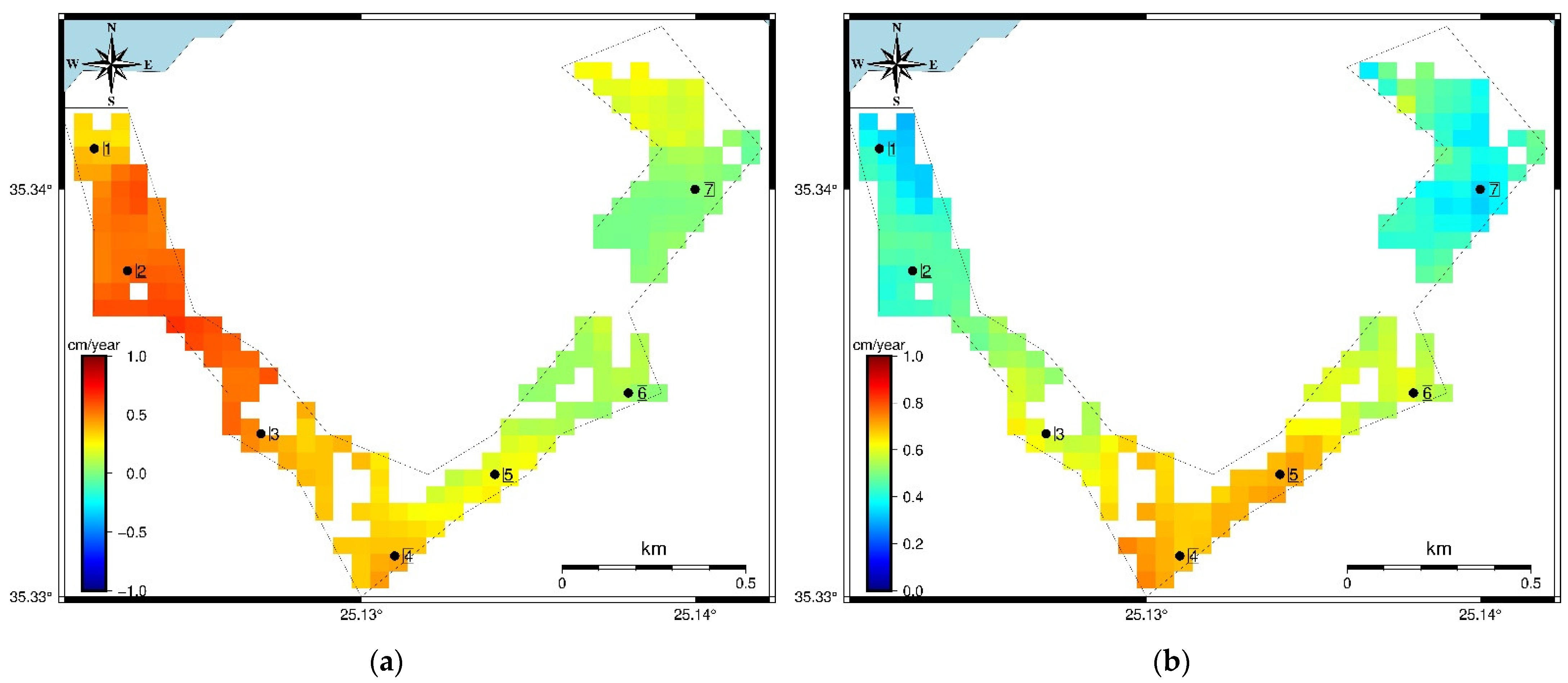
4.1. The 2D Co-Seismic Deformations
4.1.1. GACOS Corrections
4.1.2. The UD and EW Deformations of the Arkalochori Earthquake
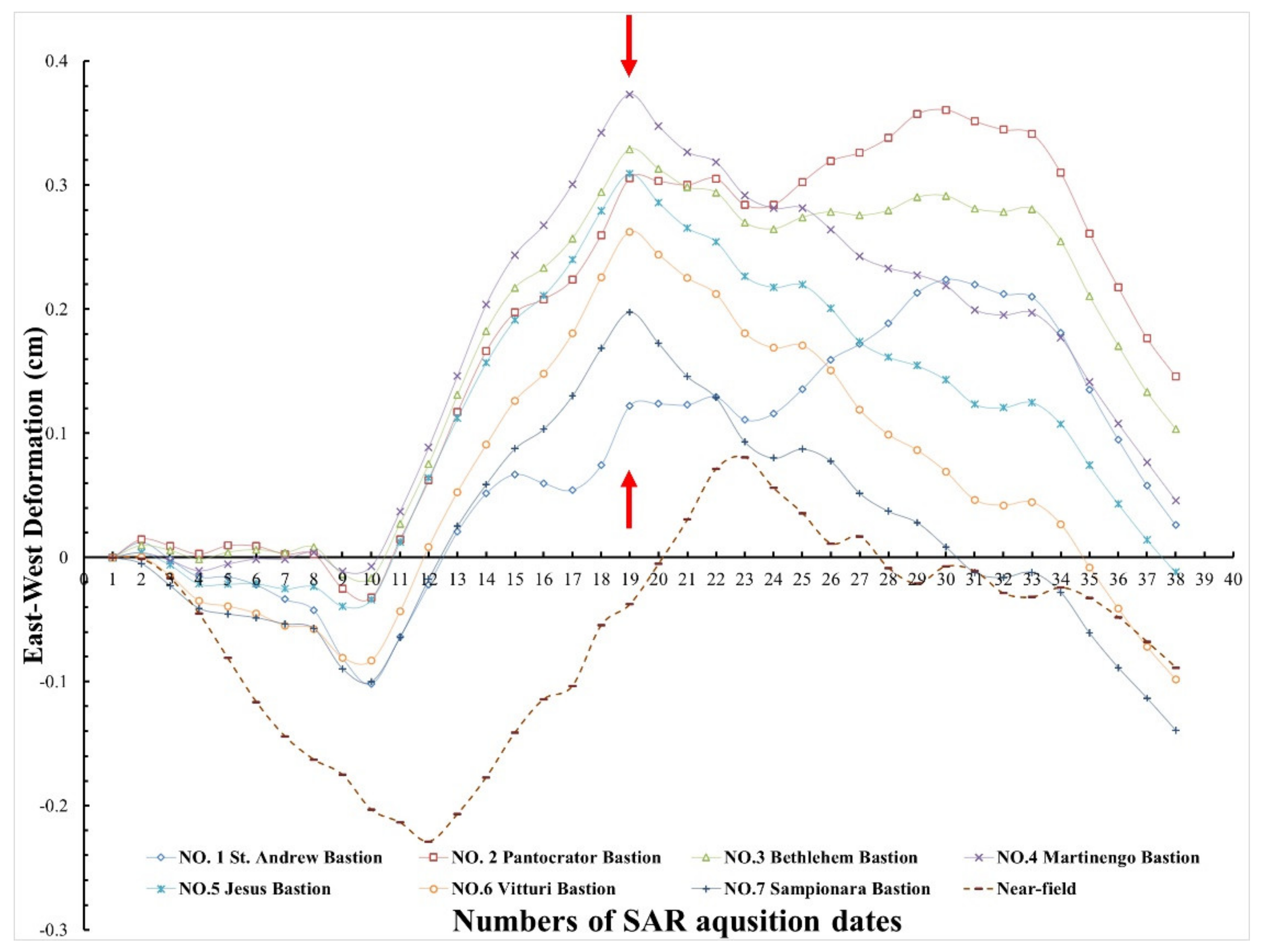
4.2. InSAR Time-Series Measurements
4.2.1. Interferogram Stacks
4.2.2. MSBAS Results
5. Discussion
6. Conclusions
Author Contributions
Funding
Data Availability Statement
Acknowledgments
Conflicts of Interest
References
- Chen, F.L.; Guo, H.D.; Tapete, D.; Masini, N.; Cigna, F.; Lasaponara, R.; Piro, S.; Lin, H.; Ma, P.F. Interdisciplinary approaches based on imaging radar enable cutting-edge cultural heritage applications. Natl. Sci. Rev. 2021, 8, 2. [Google Scholar] [CrossRef]
- Tapete, D.; Cigna, F. InSAR data for geohazard assessment in UNESCO World Heritage sites: Stateof-the-art and perspectives in the Copernicus era. Int. J. Appl. Earth Obs. Geoinf. 2017, 63, 24–32. [Google Scholar] [CrossRef]
- Themistocleous, K.; Danezis, C.; Gikas, V. Monitoring ground deformation of cultural heritage sites using SAR and geodetic techniques: The case study of Choirokoitia, Cyprus. Appl. Geomat. 2021, 13, 37–49. [Google Scholar] [CrossRef]
- Reale, D.; Noviello, C.; Verde, S.; Cascini, L.; Terracciano, G.; Arena, L. A multi-disciplinary approach for the damage analysis of cultural heritage: The case study of the St. Gerlando Cathedral in Agrigento. Remote Sens. Environ. 2019, 235, 12. [Google Scholar] [CrossRef]
- Pastonchi, L.; Barra, A.; Monserrat, O.; Luzi, G.; Solari, L.; Tofani, V. Satellite Data to Improve the Knowledge of Geohazards in World Heritage Sites. Remote Sens. 2018, 10, 992. [Google Scholar] [CrossRef]
- Pavlova, I.; Makarigakis, A.; Depret, T.; Jomelli, V. Global overview of the geological hazard exposure and disaster risk awareness at world heritage sites. J. Cult. Herit. 2017, 28, 151–157. [Google Scholar] [CrossRef]
- Vassilakis, E.; Kaviris, G.; Kapetanidis, V.; Papageorgiou, E.; Foumelis, M.; Konsolaki, A.; Petrakis, S.; Evangelidis, C.P.; Alexopoulos, J.; Karastathis, V.; et al. The 27 September 2021 Earthquake in Central Crete (Greece)-Detailed Analysis of the Earthquake Sequence and Indications for Contemporary Arc-Parallel Extension to the Hellenic Arc. Appl. Sci. 2022, 12, 2815. [Google Scholar] [CrossRef]
- Chen, F.L.; Guo, H.D.; Ishwaran, N.; Liu, J.; Wang, X.Y.; Zhou, W.; Tang, P.P. Understanding the relationship between the water crisis and sustainability of the Angkor World Heritage site. Remote Sens. Environ. 2019, 232, 12. [Google Scholar] [CrossRef]
- Chen, F.L.; Guo, H.D.; Ma, P.F.; Lin, H.; Wang, C.; Ishwaran, N.; Hang, P. Radar interferometry offers new insights into threats to the Angkor site. Sci. Adv. 2017, 3, 8. [Google Scholar] [CrossRef]
- Cigna, F.; Lasaponara, R.; Masini, N.; Milillo, P.; Tapete, D. Persistent Scatterer Interferometry Processing of COSMO-SkyMed StripMap HIMAGE Time Series to Depict Deformation of the Historic Centre of Rome, Italy. Remote Sens. 2014, 6, 12593–12618. [Google Scholar] [CrossRef]
- Cigna, F.; Tapete, D. Tracking Human-Induced Landscape Disturbance at the Nasca Lines UNESCO World Heritage Site in Peru with COSMO-SkyMed InSAR. Remote Sens. 2018, 10, 572. [Google Scholar] [CrossRef]
- Drougkas, A.; Verstrynge, E.; Van Balen, K.; Shimoni, M.; Croonenborghs, T.; Hayen, R.; Declercq, P.-Y. Country-scale InSAR monitoring for settlement and uplift damage calculation in architectural heritage structures. Struct. Health Monit. 2020, 2020, 1475921720942120. [Google Scholar] [CrossRef]
- Nappo, N.; Peduto, D.; Polcari, M.; Livio, F.; Ferrario, M.F.; Comerci, V.; Stramondo, S.; Michetti, A.M. Subsidence in Como historic centre (northern Italy): Assessment of building vulnerability combining hydrogeological and stratigraphic features, Cosmo-SkyMed InSAR and damage data. Int. J. Disaster Risk Reduct. 2021, 56, 16. [Google Scholar] [CrossRef]
- Ma, P.F.; Lin, H.; Wang, W.X.; Yu, H.W.; Chen, F.L.; Jiang, L.M.; Zhou, L.F.; Zhang, Z.J.; Shi, G.Q.; Wang, J.L. Toward Fine Surveillance: A Review of Multitemporal Interferometric Synthetic Aperture Radar for Infrastructure Health Monitoring. IEEE Geosci. Remote Sens. Mag. 2022, 10, 207–230. [Google Scholar] [CrossRef]
- Tzouvaras, M.; Kouhartsiouk, D.; Agapiou, A.; Danezis, C.; Hadjimitsis, D.G. The Use of Sentinel-1 Synthetic Aperture Radar (SAR) Images and Open-Source Software for Cultural Heritage: An Example from Paphos Area in Cyprus for Mapping Landscape Changes after a 5.6 Magnitude Earthquake. Remote Sens. 2019, 11, 1766. [Google Scholar] [CrossRef]
- Agapiou, A.; Lysandrou, V. Detecting Displacements Within Archaeological Sites in Cyprus After a 5.6 Magnitude Scale Earthquake Event Through the Hybrid Pluggable Processing Pipeline (HyP3) Cloud-Based System and Sentinel-1 Interferometric Synthetic Aperture Radar (InSAR) Analysis. IEEE J. Sel. Top. Appl. Earth Observ. Remote Sens. 2020, 13, 6115–6123. [Google Scholar] [CrossRef]
- Agapiou, A. UNESCO World Heritage properties in changing and dynamic environments: Change detection methods using optical and radar satellite data. Herit. Sci. 2021, 9, 14. [Google Scholar] [CrossRef]
- Triantafyllou, I.; Karavias, A.; Koukouvelas, I.; Papadopoulos, G.A.; Parcharidis, I. The Crete Isl. (Greece) Mw6.0 Earthquake of 27 September 2021: Expecting the Unexpected. GeoHazards 2022, 3, 106–124. [Google Scholar] [CrossRef]
- Vallianatos, F.; Karakonstantis, A.; Michas, G.; Pavlou, K.; Kouli, M.; Sakkas, V. On the Patterns and Scaling Properties of the 2021–2022 Arkalochori Earthquake Sequence (Central Crete, Greece) Based on Seismological, Geophysical and Satellite Observations. Appl. Sci. 2022, 12, 7716. [Google Scholar] [CrossRef]
- Peleli, S.; Kouli, M.; Vallianatos, F. Satellite-Observed Thermal Anomalies and Deformation Patterns Associated to the 2021, Central Crete Seismic Sequence. Remote Sens. 2022, 14, 3413. [Google Scholar] [CrossRef]
- Ganas, A.; Hamiel, Y.; Serpetsidaki, A.; Briole, P.; Valkaniotis, S.; Fassoulas, C.; Piatibratova, O.; Kranis, H.; Tsironi, V.; Karamitros, I.; et al. The Arkalochori Mw = 5.9 Earthquake of 27 September 2021 Inside the Heraklion Basin: A Shallow, Blind Rupture Event Highlighting the Orthogonal Extension of Central Crete. Geosciences 2022, 12, 220. [Google Scholar] [CrossRef]
- Crosetto, M.; Monserrat, O.; Cuevas-Gonzalez, M.; Devanthery, N.; Crippa, B. Persistent Scatterer Interferometry: A review. ISPRS-J. Photogramm. Remote Sens. 2016, 115, 78–89. [Google Scholar] [CrossRef]
- Yu, C.; Li, Z.H.; Penna, N.T. Interferometric synthetic aperture radar atmospheric correction using a GPS-based iterative tropospheric decomposition model. Remote Sens. Environ. 2018, 204, 109–121. [Google Scholar] [CrossRef]
- Yu, C.; Li, Z.H.; Penna, N.T.; Crippa, P. Generic Atmospheric Correction Model for Interferometric Synthetic Aperture Radar Observations. J. Geophys. Res.-Solid Earth 2018, 123, 9202–9222. [Google Scholar] [CrossRef]
- Yu, C.; Penna, N.T.; Li, Z.H. Generation of real-time mode high-resolution water vapor fields from GPS observations. J. Geophys. Res.-Atmos. 2017, 122, 2008–2025. [Google Scholar] [CrossRef]
- Alinia, H.S.; Tiampo, K.F.; Samsonov, S.V.; Gonzalez, P.J. Modelling the elevation-dependent seasonal amplitude of tropospheric delays in GPS time-series using DInSAR and meteorological data. Geophys. J. Int. 2019, 216, 676–691. [Google Scholar] [CrossRef]
- Liu, X.J.; Zhao, C.Y.; Zhang, Q.; Yin, Y.P.; Lu, Z.; Samsonov, S.; Yang, C.S.; Wang, M.; Tomas, R. Three-dimensional and long-term landslide displacement estimation by fusing C- and L-band SAR observations: A case study in Gongjue County, Tibet, China. Remote Sens. Environ. 2021, 267, 20. [Google Scholar] [CrossRef]
- Samsonov, S. Three-dimensional deformation time series of glacier motion from multiple-aperture DInSAR observation. J. Geod. 2019, 93, 2651–2660. [Google Scholar] [CrossRef]
- Samsonov, S.; Baryakh, A. Estimation of Deformation Intensity above a Flooded Potash Mine Near Berezniki (Perm Krai, Russia) with SAR Interferometry. Remote Sens. 2020, 12, 3215. [Google Scholar] [CrossRef]
- Samsonov, S.; Dille, A.; Dewitte, O.; Kervyn, F.; d’Oreye, N. Satellite interferometry for mapping surface deformation time series in one, two and three dimensions: A new method illustrated on a slow-moving landslide. Eng. Geol. 2020, 266, 13. [Google Scholar] [CrossRef]
- Samsonov, S.; d’Oreye, N. Multidimensional time-series analysis of ground deformation from multiple InSAR data sets applied to Virunga Volcanic Province. Geophys. J. Int. 2012, 191, 1095–1108. [Google Scholar] [CrossRef]
- Samsonov, S.; d’Oreye, N.; Smets, B. Ground deformation associated with post-mining activity at the French-German border revealed by novel InSAR time series method. Int. J. Appl. Earth Obs. Geoinf. 2013, 23, 142–154. [Google Scholar] [CrossRef]
- Samsonov, S.V.; d’Oreye, N. Multidimensional Small Baseline Subset (MSBAS) for Two-Dimensional Deformation Analysis: Case Study Mexico City. Can. J. Remote Sens. 2017, 43, 318–329. [Google Scholar] [CrossRef]
- Samsonov, S.V.; d’Oreye, N.; Gonzalez, P.J.; Tiampo, K.F.; Ertolahti, L.; Clague, J.J. Rapidly accelerating subsidence in the Greater Vancouver region from two decades of ERS-ENVISAT-RADARSAT-2 DInSAR measurements. Remote Sens. Environ. 2014, 143, 180–191. [Google Scholar] [CrossRef]
- Morishita, Y.; Kobayashi, T.; Yarai, H. Three-dimensional deformation mapping of a dike intrusion event in Sakurajima in 2015 by exploiting the right- and left-looking ALOS-2 InSAR. Geophys. Res. Lett. 2016, 43, 4197–4204. [Google Scholar] [CrossRef]
- Agram, P.S.; Gurrola, E.M.; Lavalle, M.; Sacco, G.F.; Rosen, P.A. The InSAR Scientific Computing Environment (ISCE): An Earth Science SAR Processing Framework, Toolbox, and Foundry. In Proceedings of the Agu Fall Meeting, San Francisco, CA, USA, 16 December 2016. [Google Scholar]
- Goldstein, R.M.; Werner, C.L. Radar interferogram filtering for geophysical applications. Geophys. Res. Lett. 1998, 25, 4035–4038. [Google Scholar] [CrossRef]
- Goldstein, R.M.; Zebker, H.A.; Werner, C.L. Satellite radar interferometry: Two-dimensional phase unwrapping. Radio Sci. 1988, 23, 713–720. [Google Scholar] [CrossRef]
- Delbridge, B.G.; Burgmann, R.; Fielding, E.; Hensley, S.; Schulz, W.H. Three-dimensional surface deformation derived from airborne interferometric UAVSAR: Application to the Slumgullion Landslide. J. Geophys. Res.-Solid Earth 2016, 121, 3951–3977. [Google Scholar] [CrossRef]
- Zhang, Z.Y.; Lou, Y.D.; Zhang, W.X.; Wang, H.; Zhou, Y.Z.; Bai, J.N. On the Assessment GPS-Based WRFDA for InSAR Atmospheric Correction: A Case Study in Pearl River Delta Region of China. Remote Sens. 2021, 13, 3280. [Google Scholar] [CrossRef]
- Tikhonov, A.N.; Arsenin, V.Y. Solution of Ill-Posed Problem; V.H. Winston and Sons: New York, NY, USA, 1977. [Google Scholar]
- Chen, C.W.; Zebker, H.A. Phase unwrapping for large SAR interferograms: Statistical segmentation and generalized network models. IEEE Trans. Geosci. Remote Sens. 2002, 40, 1709–1719. [Google Scholar] [CrossRef]
- Sandwell, D.; Mellors, R.; Tong, X.; Wei, M.; Wessel, P. Open radar interferometry software for mapping surface Deformation. Eos Trans. AGU 2011, 92, 234. [Google Scholar] [CrossRef]
- Zebker, H. Accuracy of a Model-Free Algorithm for Temporal InSAR Tropospheric Correction. Remote Sens. 2021, 13, 409. [Google Scholar] [CrossRef]
- Liao, T.H.; Simard, M.; Denbina, M.; Lamb, M.P. Monitoring Water Level Change and Seasonal Vegetation Change in the Coastal Wetlands of Louisiana Using L-Band Time-Series. Remote Sens. 2020, 12, 2351. [Google Scholar] [CrossRef]
- Zhu, M.; Zeng, Q.M.; Jiao, J. Quantitative assessment to the impact of InSAR ionospheric and tropospheric corrections on source parameter modelling: Application to the 4th nuclear test, North Korea. Geophys. J. Int. 2021, 224, 86–99. [Google Scholar] [CrossRef]
- Fialko, Y. Probing the mechanical properties of seismically active crust with space geodesy: Study of the coseismic deformation due to the 1992 M(w)7.3 Landers (southern California) earthquake. J. Geophys. Res.-Solid Earth 2004, 109, 19. [Google Scholar] [CrossRef]
- Hu, J.; Liu, J.H.; Li, Z.W.; Zhu, J.J.; Wu, L.X.; Sun, Q.; Wu, W.Q. Estimating three-dimensional coseismic deformations with the SM-VCE method based on heterogeneous SAR observations: Selection of homogeneous points and analysis of observation combinations. Remote Sens. Environ. 2021, 255, 16. [Google Scholar] [CrossRef]
- Berardino, P.; Fornaro, G.; Lanari, R.; Sansosti, E. A new algorithm for surface deformation monitoring based on small baseline differential SAR interferograms. IEEE Trans. Geosci. Remote Sens. 2002, 40, 2375–2383. [Google Scholar] [CrossRef]
- Yu, C.; Li, Z.H.; Penna, N.T. Triggered afterslip on the southern Hikurangi subduction interface following the 2016 Kaikura earthquake from InSAR time series with atmospheric corrections. Remote Sens. Environ. 2020, 251, 17. [Google Scholar] [CrossRef]
- Samsonov, S.; Tiampo, K.; Cassotto, R. Measuring the state and temporal evolution of glaciers in Alaska and Yukon using synthetic-aperture-radar-derived (SAR-derived) 3D time series of glacier surface flow. Cryosphere 2021, 15, 4221–4239. [Google Scholar] [CrossRef]
- Atzori, S.; Manunta, M.; Fornaro, G.; Ganas, A.; Salvi, S. Postseismic displacement of the 1999 Athens earthquake retrieved by the Differential Interferometry by Synthetic Aperture Radar time series. J. Geophys. Res.-Solid Earth 2008, 113, 14. [Google Scholar] [CrossRef]
- Briole, P.; Elias, P.; Parcharidis, I.; Bignami, C.; Benekos, G.; Samsonov, S.; Kyriakopoulos, C.; Stramondo, S.; Chamot-Rooke, N.; Drakatou, M.L.; et al. The seismic sequence of January-February 2014 at Cephalonia Island (Greece): Constraints from SAR interferometry and GPS. Geophys. J. Int. 2015, 203, 1528–1540. [Google Scholar] [CrossRef][Green Version]
- De Novellis, V.; Convertito, V.; Valkaniotis, S.; Casu, F.; Lanari, R.; Tobar, M.F.M.; Pino, N.A. Coincident locations of rupture nucleation during the 2019 Le Teil earthquake, France and maximum stress change from local cement quarrying. Commun. Earth Environ. 2020, 1, 10. [Google Scholar] [CrossRef]
- Ganas, A.; Kourkouli, P.; Briole, P.; Moshou, A.; Elias, P.; Parcharidis, I. Coseismic Displacements from Moderate-Size Earthquakes Mapped by Sentinel-1 Differential Interferometry: The Case of February 2017 Gulpinar Earthquake Sequence (Biga Peninsula, Turkey). Remote Sens. 2018, 10, 1089. [Google Scholar] [CrossRef]
- Hamiel, Y.; Baer, G.; Kalindekafe, L.; Dombola, K.; Chindandali, P. Seismic and aseismic slip evolution and deformation associated with the 2009-2010 northern Malawi earthquake swarm, East African Rift. Geophys. J. Int. 2012, 191, 898–908. [Google Scholar] [CrossRef]
- Hamiel, Y.; Fialko, Y. Structure and mechanical properties of faults in the North Anatolian Fault system from InSAR observations of coseismic deformation due to the 1999 Izmit (Turkey) earthquake. J. Geophys. Res.-Solid Earth 2007, 112, 12. [Google Scholar] [CrossRef]
- Ilieva, M.; Briole, P.; Ganas, A.; Dimitrov, D.; Elias, P.; Mouratidis, A.; Charara, R. Fault plane modelling of the 2003 August 14 Lefkada Island (Greece) earthquake based on the analysis of ENVISAT SAR interferograms. Tectonophysics 2016, 693, 47–65. [Google Scholar] [CrossRef]
- Melgar, D.; Ganas, A.; Taymaz, T.; Valkaniotis, S.; Crowell, B.W.; Kapetanidis, V.; Tsironi, V.; Yolsal-Cevikbilen, S.; Ocalan, T. Rupture kinematics of 2020 January 24 M-w 6.7 Doganyol-Sivrice, Turkey earthquake on the East Anatolian Fault Zone imaged by space geodesy. Geophys. J. Int. 2020, 223, 862–874. [Google Scholar] [CrossRef]
- Taymaz, T.; Ganas, A.; Yolsal-Cevikbilen, S.; Vera, F.; Eken, T.; Erman, C.; Keles, D.; Kapetanidis, V.; Valkaniotis, S.; Karasante, I.; et al. Source Mechanism and Rupture Process of the 24 January 2020 Mw 6.7 Doganyol-Sivrice Earthquake obtained from Seismological Waveform Analysis and Space Geodetic Observations on the East Anatolian Fault Zone (Turkey). Tectonophysics 2021, 804, 29. [Google Scholar] [CrossRef]
- Neokosmidis, S.; Elias, P.; Parcharidis, I.; Briole, P. Deformation estimation of an earth dam and its relation with local earthquakes, by exploiting multitemporal synthetic aperture radar interferometry: Mornos dam case (Central Greece). J. Appl. Remote Sens. 2016, 10, 16. [Google Scholar] [CrossRef]
- Zhou, W.; Chen, F.L.; Guo, H.D. Differential Radar Interferometry for Structural and Ground Deformation Monitoring: A New Tool for the Conservation and Sustainability of Cultural Heritage Sites. Sustainability 2015, 7, 1712–1729. [Google Scholar] [CrossRef]
- Kirui, P.K.; Reinosch, E.; Isya, N.; Riedel, B.; Gerke, M. Mitigation of Atmospheric Artefacts in Multi Temporal InSAR: A Review. PFG-J. Photogramm. Remote Sens. Geoinf. Sci. 2021, 89, 251–272. [Google Scholar] [CrossRef]
- Li, Z.W.; Cao, Y.M.; Wei, J.C.; Duan, M.; Wu, L.X.; Hou, J.X.; Zhu, J.J. Time-series InSAR ground deformation monitoring: Atmospheric delay modeling and estimating. Earth-Sci. Rev. 2019, 192, 258–284. [Google Scholar] [CrossRef]
- Murray, K.D.; Bekaert, D.P.S.; Lohman, R.B. Tropospheric corrections for InSAR: Statistical assessments and applications to the Central United States and Mexico. Remote Sens. Environ. 2019, 232, 12. [Google Scholar] [CrossRef]


| Platform (Mode) | Track/Frame | Reference/Repeat Date (YYYYMMDD) | Incidence Angle (°) | Heading 1 (°) | Perpendicular Baseline (m) |
|---|---|---|---|---|---|
| Sentinel-1A (TOPS) Ascending | 102/113 | 17 September 2021/ 29 September 2021 | 44.002 | −12.957 | 69.879 |
| 102/108 | |||||
| Sentinel-1A (TOPS) Descending | 109/476 | 18 September 2021/ 30 September 2021 | 33.927 | −166.997 | −22.354 |
| Interferogram Stack | Incidence Angle (°) | Heading 1 (°) | Temporal Coverage | Number of SAR Images | Number of Interferograms |
|---|---|---|---|---|---|
| Sentinel-1A (TOPS) Ascending Track 029 | 34.040 | −13.078 | 6 October 2021–22 May 2022 | 20 | 157 |
| Sentinel-1A (TOPS) Descending Track 109 | 33.927 | −166.997 | 30 September 2021–16 May 2022 | 20 | 152 |
| Total | / | / | 6 October 2021–16 May 2022 | 40 2 | 307 |
| Point | EW Deformation 1 (cm) | UD Deformation 2 (cm) |
|---|---|---|
| 1 St. Andrew Bastion | −0.080 | −0.241 |
| 2 Pantocrator Bastion | −0.186 | −0.244 |
| 3 Bethlehem Bastion | −0.372 | −0.114 |
| 4 Martinengo Bastion | −0.029 | −0.239 |
| 5 Jesus Bastion | −0.044 | −0.346 |
| 6 Vitturi Bation | 0.088 | −0.181 |
| 7 Sampionara Bastion | 0.236 | −0.066 |
| The near-field area | 6.223 | −16.489 |
Publisher’s Note: MDPI stays neutral with regard to jurisdictional claims in published maps and institutional affiliations. |
© 2022 by the authors. Licensee MDPI, Basel, Switzerland. This article is an open access article distributed under the terms and conditions of the Creative Commons Attribution (CC BY) license (https://creativecommons.org/licenses/by/4.0/).
Share and Cite
Zhu, M.; Chen, F.; Zhou, W.; Lin, H.; Parcharidis, I.; Luo, J. Two-Dimensional InSAR Monitoring of the Co- and Post-Seismic Ground Deformation of the 2021 Mw 5.9 Arkalochori (Greece) Earthquake and Its Impact on the Deformations of the Heraklion City Wall Relic. Remote Sens. 2022, 14, 5212. https://doi.org/10.3390/rs14205212
Zhu M, Chen F, Zhou W, Lin H, Parcharidis I, Luo J. Two-Dimensional InSAR Monitoring of the Co- and Post-Seismic Ground Deformation of the 2021 Mw 5.9 Arkalochori (Greece) Earthquake and Its Impact on the Deformations of the Heraklion City Wall Relic. Remote Sensing. 2022; 14(20):5212. https://doi.org/10.3390/rs14205212
Chicago/Turabian StyleZhu, Meng, Fulong Chen, Wei Zhou, Hui Lin, Issaak Parcharidis, and Jin Luo. 2022. "Two-Dimensional InSAR Monitoring of the Co- and Post-Seismic Ground Deformation of the 2021 Mw 5.9 Arkalochori (Greece) Earthquake and Its Impact on the Deformations of the Heraklion City Wall Relic" Remote Sensing 14, no. 20: 5212. https://doi.org/10.3390/rs14205212
APA StyleZhu, M., Chen, F., Zhou, W., Lin, H., Parcharidis, I., & Luo, J. (2022). Two-Dimensional InSAR Monitoring of the Co- and Post-Seismic Ground Deformation of the 2021 Mw 5.9 Arkalochori (Greece) Earthquake and Its Impact on the Deformations of the Heraklion City Wall Relic. Remote Sensing, 14(20), 5212. https://doi.org/10.3390/rs14205212