Article

A Modified Shape Model Incorporating Continuous Accumulated Growing Degree Days for Phenology Detection of Early Rice

1
College of Surveying and Geo-Informatics, Tongji University, Shanghai 200092, China
2
Shanghai Key Laboratory for Planetary Mapping and Remote Sensing for Deep Space Exploration, Tongji University, Shanghai 200092, China
3
Frontiers Science Center for Intelligent Autonomous Systems, Tongji University, Shanghai 201210, China
*
Author to whom correspondence should be addressed.
Remote Sens. 2022, 14(21), 5337; https://doi.org/10.3390/rs14215337
Submission received: 19 September 2022 / Revised: 21 October 2022 / Accepted: 22 October 2022 / Published: 25 October 2022
(This article belongs to the Special Issue Remote Sensing in Land Use and Management)

Abstract

:
Using a shape model (SM) is a typical method to determine the phenological phases of crops with long-time-series satellite remote sensing data. The average AGDD-based shape model (AAGDD-SM) takes temperature into account compared to SM, however, the commonly used daily average temperature is not sufficient to determine the exact AGDD owing to the possibly significant changes in temperatures throughout the day. In this paper, a modified shape model was proposed for the better estimation of phenological dates and it is incorporated into the continuous AGDD (CAGDD) which was calculated based on temperatures from a continuous 24 h within a day, different from the calendar day or the average AGDD indicators. In this study, the CAGDD replaced the abscissa of the NDVI growth curve over a 5-year period (2014 to 2018, excluding 2015) for a test site of early rice in Jiangxi province of China. Four key phenological phases, including the reviving, tillering, heading and anthesis phases, were selected and determined with reference to the field-observed phenological data. The results show that compared with the AAGDD-SM, the method proposed in this paper has basically improved the prediction of each phenological period. For those cases where the average temperature is lower than the minimum temperatures (K1) but the effective accumulated temperature is not zero, more accurate AGDD can be calculated according to the method in this paper.

Graphical Abstract

1. Introduction

The phenology of plants refers to a series of seasonal regular changes in the growth and development that adapt to the climate, such as germination, branching out, leaf development, flowering, fruiting, defoliation, and dormancy, and the corresponding dynamic phases of plants, which are called the phenological phases [1]. Phenology was widely applied in the agricultural field; accurate phenological information can help to develop reasonable agricultural production plans and facilitate crop cultivation and pest control [2,3,4,5,6,7,8]. In addition, the phenological phase is also one of the indispensable parameters for crop yield estimation [9,10,11,12,13,14,15].
Generally, there are three methods for observing the phenological phases [16]: manual observation, near-ground sensors and satellite-based remote sensing. Manual observation is the most common way for phenological phase determination over the past centuries and several phenological observation networks have been established across the world, such as the National Phenology Network (NPN) in the United States and the China Phenological Observation Network (CPON) in China [17,18,19]. Although the phenological network can provide accurate phenological information, it is time-consuming and lacks the capability of wide coverage. Near-surface sensors are able to conduct the observation for a long duration, however, it is also not applicable for regional or global missions and the obtained data are not accessible to all researchers [20,21]. Therefore, satellite-based remote sensing data have become an important resource for researchers to monitor the phenology of crops [22,23,24,25].
Studies of phenological phase detection with satellite remote sensing data have been conducted by researchers over decades and numerous algorithms have been proposed, such as threshold-based methods [26,27,28], phenological indexes [29,30,31], shape models, and so on [32,33]. The principle of threshold-based methods is to set a fixed value for a specific phenological period in advance, and then extract the phenological period from the vegetation indexes (VI) curve according to these values. Many VI curves obtained from satellite remote sensing observation have been extracted by threshold-based methods [34,35,36]. Although this method is simple, the selected threshold has no potential biophysical significance, and a single threshold may not be suitable for various crops in different areas. Phenological index-based methods extract phenology according to the changing characteristics of the VI curve. There are many applications of phenological indexes combined with remote sensing images [31,37]. However, this method is easily disturbed by local outliers. In recent years, the shape model has attracted much attention owing to its ability to accurately extract phenological phases. Generally, the shape model is generated by averaging the annual growth trajectory curves which are obtained by fitting the calculated sequential VI. The shape of the model matches the growth curve of a single year through the curve obtained after averaging, which can eliminate the interference of abnormal values caused by the climate difference between years using traditional methods. Averaging is used to reduce the influence of local outliers of curves in specific years. Given the generated shape model and its corresponding preliminary-defined phenological parameters, the annual phenological dates can be determined by matching the shape model with the fitted VI curve. The shape model was first proposed by Sakamoto [38] for detecting maize and soybean phenology with time-series MODIS data under the assumption that the growth rate of the crop was correlated with the growth time. Therefore, the calendar day was used as the independent variable with the VI when fitting the growth trajectory curves. However, the calendar day may not be a suitable indicator to measure the growth situation of crops. According to the law of accumulated growing degree days (AGDD) of crops [39], the crops can only continue to grow under the circumstance that a certain accumulative heat is reached for a certain phenological phase. Moreover, the AGDD required for each growth stage of crops is usually constant [40,41]. The transformation of different phenological phases needs to meet their respective AGDD. Therefore, the AGDD indicator is better than the calendar day to generate the growth trajectory curves and shape model. Therefore, it is necessary to calculate the value of AGDD accurately. Zeng et al. [42] incorporated the influence of environmental factors into the shape model and used the nonlinear model to calculate the accumulated photothermal time of crops as the independent variable, to better fit the shape model, thus achieving a higher phenological period extraction accuracy. Due to the computational complexity of the nonlinear model, Zhou et al. [43] introduced the AGDD, which was calculated based on the daily average temperature, to replace the calendar day in shape model generation. In this way, higher accuracy can be achieved for phenological phase extraction. However, the daily average temperature is still not sufficient to determine the exact AGDD owing to the possibly significant changes in temperatures throughout the day [44]. For example, for a specific date, the average temperature is less than the minimum temperature. According to the calculation of the average temperature method, the GDD on that day is 0, but the plants have not stopped growing.
In this paper, a modified shape model was proposed for the better estimation of phenological dates, and it incorporated the continuous AGDD (namely CAGDD) which was calculated based on the temperatures of a continuous 24 h within a day, which is different from the calendar day or the average AGDD indicators. The advantage of this method is to use the whole-day duration combined with the sine method to calculate a more accurate AGDD. It is believed that the CAGDD can depict the contribution of temperature factors appropriately and reflect the growth of crops accurately. Compared with CD-SM and AAGDD-SM, the accuracy of CAGDD-SM is obviously improved, and this method can extract phenology more accurately. In addition, in order to prove the rationality of the combination of SM and the sine method in calculating AGDD, this paper also made two comparative experiments, which fully demonstrated the reasonableness of the proposed CAGDD-SM.

2. Materials and Methods

2.1. Materials

2.1.1. Study Area

The research area (117°4′43.38″E, 28°57′24.96″N) is located in Leping city, Jiangxi Province of China, covering an area of about 13 hectares (Figure 1). Rice is planted all year round in rotation of early rice and late rice.
Taking early rice as an example, the transplanting period of early rice usually starts from the end of April to the beginning of May, and early rice matures at the end of July (due to climate reasons, early rice is transplanted while not sown directly). The local early rice (Jiangxi Zhongzao 33) did not change in variety from 2013–2018. The reason for choosing this area was that this paddy field is the closest to the phenological observation station set by the Leping city Meteorological Bureau, which could therefore provide accurate ground observation phenological information of early rice. The observation station is located southeast of the paddy field, about 1.5 km away. Compared with previous research, the most prominent characteristic of this study area is that the selected area is not a standard and unified experimental field, but an ordinary piece of cultivated land, which is more practical. In addition, the Leping city Meteorological Bureau also provided daily hourly temperature data from 2014 to 2018. These years were consistent with the observation data of phenology that they could provide. The reliability of the data has been validated by professional departments.

2.1.2. Remote Sensing Data

The remote sensing data used in this paper was MODIS daily products-MOD09GQ (collection6, title: h28v06, 250 m) and MOD09GA (collection 6, title: h28v06, 500 m) from April to July 2014–2018. The main purpose of the MOD09GA products was to generate cloud masks to eliminate MOD09GQ products in which the study area was often covered by clouds. The mask file was generated by using the quality evaluation band in MOD09GA and then resampled to the same resolution as MOD09GQ. Finally, the cloud-containing images of MOD09GQ products in the study area were filtered by the mask file. Finally, the cloudless image of the study area could be obtained to generate the growth curve. The NDVI [45,46,47] values were calculated using band 1 (red band) and band 2 (near the red band) in MOD09GQ (Equation (1)). Taking the images of the study area in 2014 as an example, Figure 2 gives the NDVI images at different imaging times and it is shown that that the brighter pixels, which indicate higher NDVI values, can be observed in July compared to that in April.
N D V I = ( ρ n i r ρ r e d ) / ( ρ n i r + ρ r e d )

2.2. Methods

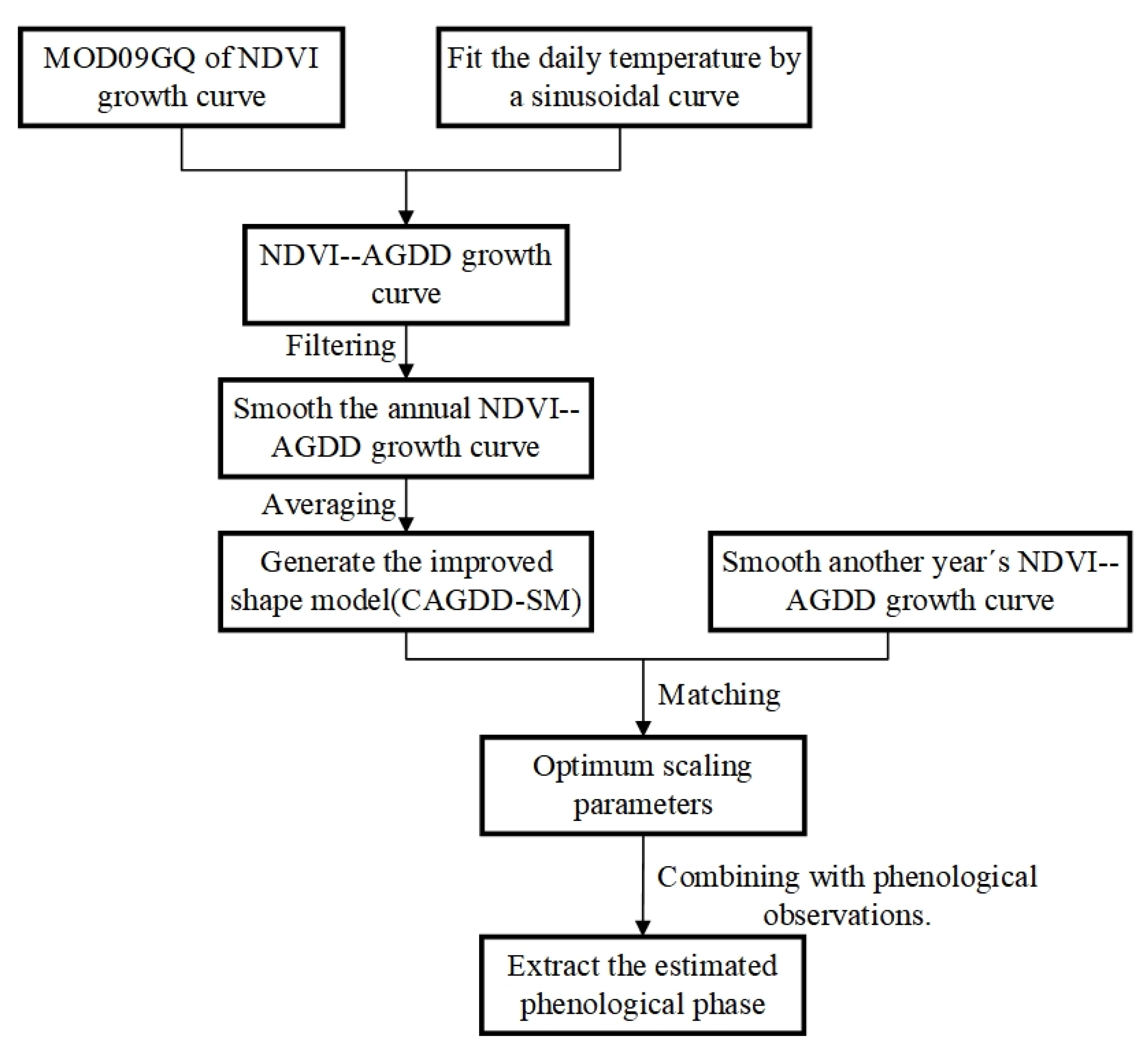
Cloud detection was conducted on the daily MOD09GQ product obtained from April to July between 2014 and 2018, and seventy-seven images were left (2015 was excluded due to the existence of too many cloudy images). The framework of the proposed method was shown in Figure 3. Firstly, the AGDD value for a certain day was obtained by the sine fitting method from the continuous 24 h temperatures, and the NDVI-AGDD growth curve was obtained in which the AGDD value was the independent variable and the NDVI value was the dependent variable. Then this NDVI-AGDD growth curve was smoothed using the double-sine fitting method [48]. These smoothed curves from different years were then further averaged to obtain the improved shape model. Finally, the generated shape model was used to match the smoothed growth curve of another year to obtain the optimal matching parameters and was then combined with the predefined phenological parameters of the shape model to estimate the phenological period of the area.

2.2.1. Calendar Day-Based Shape Model

The calendar day-based shape model [38] assumes that the growth of the crop is correlated to the growth time, and therefore utilizes the calendar day as the independent variable to fit a growth trajectory curve of the crop for each year. Furthermore, the shape model can be built from the crop’s multi-year growth curves. After that, the optimal matching parameters between the generated shape model and the growth curve for another year can be calculated, and these parameters are used to estimate the phenological dates. This kind of method mainly consists of the following steps:
(1) Given the temporal NDVI values obtained from image sequences of the study area in year i, where i [ 1 , M ] and M is the number of years to generate the shape model, the growth trajectory curve of year i can be fitted and further smoothed, as illustrated in Figure S1.
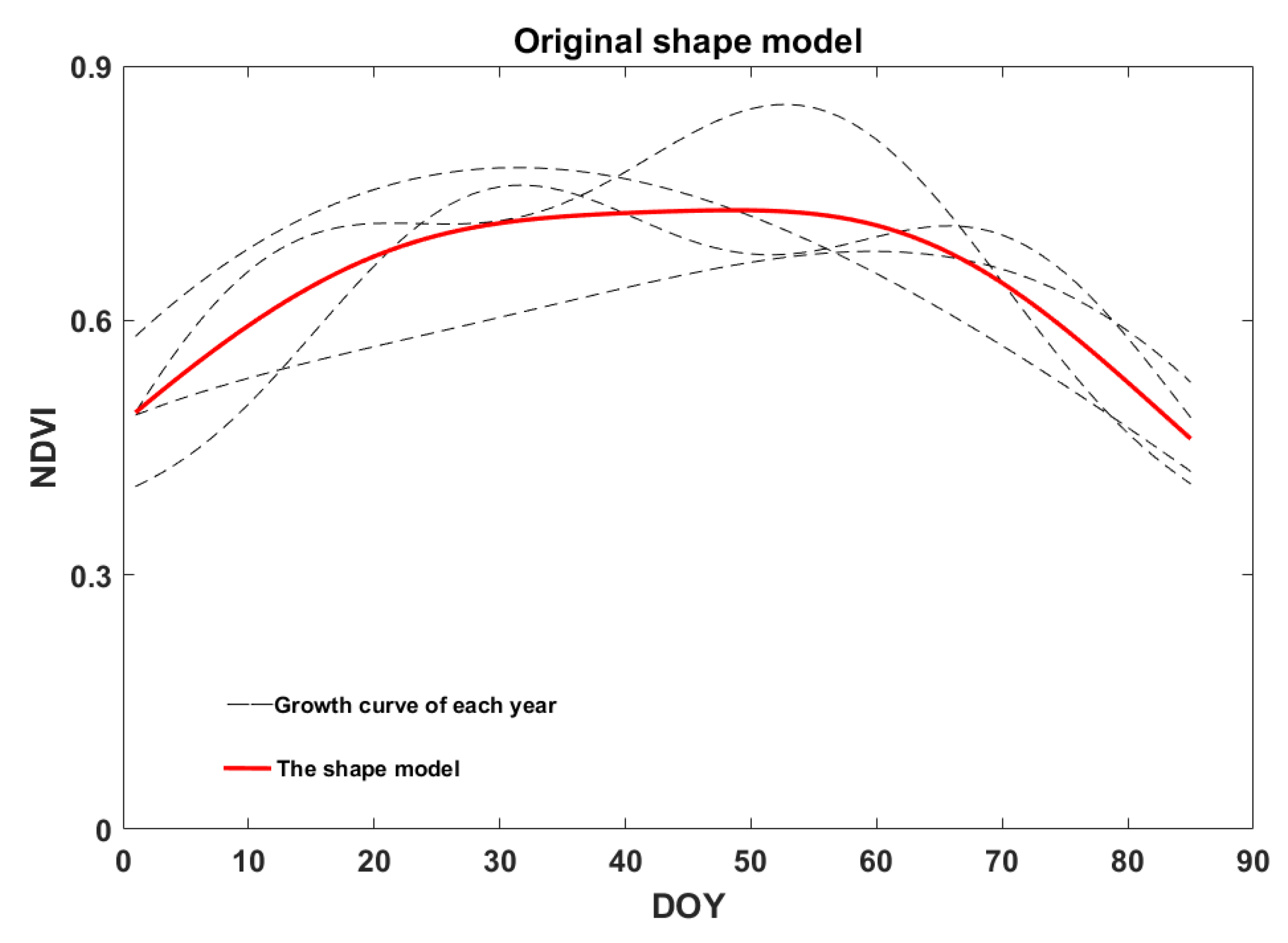
(2) The fitted curves for M years are then averaged to obtain the shape model, which can effectively suppress the inter-annual differences between the growth curves, as Figure 4 shows. With the constructed shape model, another growth curve from the target area for year j, where j [ 1 , M ] , can be matched with the shape model to generate the optimal matching parameters, as Equation (2) shows:
R M S E = [ 1 N x = 1 , 2 , 3 , N ( f ( x ) g ( x ) ) 2 ] 1 2
where x is the calendar day which is temporally resampled at equally spaced intervals and N is the corresponding number of sample points. f(x) is the growth curve from the target area for year j, and g(x) is a function of the generated shape model, as illustrated in Equation (3):
g ( x ) = y s c a l e × h ( x s c a l e × ( x + t s h i f t ) )
where h(·) is the obtained shape model, xscale, yscale and tshift are the matching parameters to be calculated by minimizing Equation (2). The search ranges for each parameter were empirically determined as follows: 0.3 < xscale < 1.5, 0.3 < yscale < 1.5 and −100 < tshift < 100.
An example of the matching procedure is demonstrated in Figure S2.
(3) With the generated optimal matching parameters, the phenological phases of year j can be determined as Equation (4).
x e s t = x s c a l e × ( X 0 s + t s h i f t )
where x e s t is an estimated phenological date of year j, and X 0 s is the preliminary defined phenological date of the shape model which can be obtained by averaging field phenological data of M years in the study area.

2.2.2. The Continuous Accumulated Growing Degree Days

According to the law of AGDD [39], the growth rate of a crop has a strong correlation with the temperature, and the crop can only continue its development state within a specific temperature range. Generally, a three-cardinal temperature system was commonly used to estimate the growth of crops in which three different temperature thresholds (K1–K3) were considered [44]. Given that the current temperature at any time is T, K 1 and K 3 are the minimum and maximum temperatures, respectively, allowing for the growth of the crop, which means the crop will not grow if T < K 1 or T > K 3 . K 2 is the optimum temperature which means the growth rate of the crop will increase with the current temperature if K 1 < T < K 2 , but remains unchanged if K 2 < T < K 3 . Table 1 gives the three-cardinal temperatures of the early rice which are provided by the local Meteorological Bureau.
Considering the influence of temperature, Zhou et al. [43] introduced the AGDD value, which was calculated from the daily average temperature, to replace the calendar day as the independent variable of the shape model to reflect the contribution of temperature to the growth of the crops (Equation (5)). This method is named as AAGDD-SM in this paper.
A G D D = k = 1 n G D D k T a v g = ( T min + T max ) / 2 { G D D = 0 T a v g K 1 G D D = T a v g T 1 K 1 < T a v g < K 3 G D D = T 3 T 1       T a v g K 3
where GDD is the calculated growing degree day value for day k, and AGDD is the sum of GDD values from day 1 to day n. T a v g is the daily average temperature, T m i n and T m a x are the lowest and highest temperatures of day k, respectively.
However, the average temperature used often underestimates the possible huge difference in the temperatures within a day. Moreover, the given assumption of Equation (5) is also flawed. For example, if the temperatures in one day are all greater than K 3 , it is deduced by Equation (5) that the crop will continue to grow, which is not supported by the AGDD law or common sense. In this paper, another criterion was designed for the proposed CAGDD-SM method according to the three-cardinal temperature system strictly, as shown in Equation (6).
{ G D D = 0 T K 1   o r   T K 3 G D D = T K 1       K 1 < T < K 2 G D D = K 2 K 1   K 2 < T < K 3
where T is the temperature at any moment of the continuous 24 h. Therefore, a modified GDD value can be calculated by fitting the temperature curve with the hourly temperatures in one day (02:00 a.m. of day k to 02:00 a.m. of day k + 1). The sine fitting method was used to generate the temperature curve by determining three key points, as explained in Figure S3. The red curve is the fitted daily temperature curve. The general procedure was as follows:
(1)
Firstly, find the time with the highest temperature in the middle period of the 24-h sequence, defined as the center point O.
(2)
Secondly, find the turning points A and B which have an equal distance from point O in 1/4 of a cycle. Given the lowest temperature in the 24-h sequence is Tmin and the temperature value of center point O as TO, assign the average value of Tmin and TO to both A and B.
(3)
With the determined three key points A, B and O, a sine curve can be obtained to represent the 24-h temperatures.
Given the fitted daily temperature curve, eight cases were considered giving the three-cardinal temperature thresholds listed in Table 1, as shown in Figure S4. The red curve is the fitted temperature curve and the daily GDD value was represented by the shaded area which can be calculated, as Equation (7) shows, taking case F as an example:
G D D = 1 24 [ t 1 t 2 ( t ( x ) K 1 ) d x + t 2 t 3 ( K 2 K 1 ) d x + t 3 t 4 ( 0 ) d x + t 4 t 5 ( K 2 K 1 ) d x + t 5 t 6 ( t ( x ) K 1 ) d x ]
where t ( x ) is the fitted temperature curve and t i is the intersection point of t ( x ) with the cardinal temperature lines.
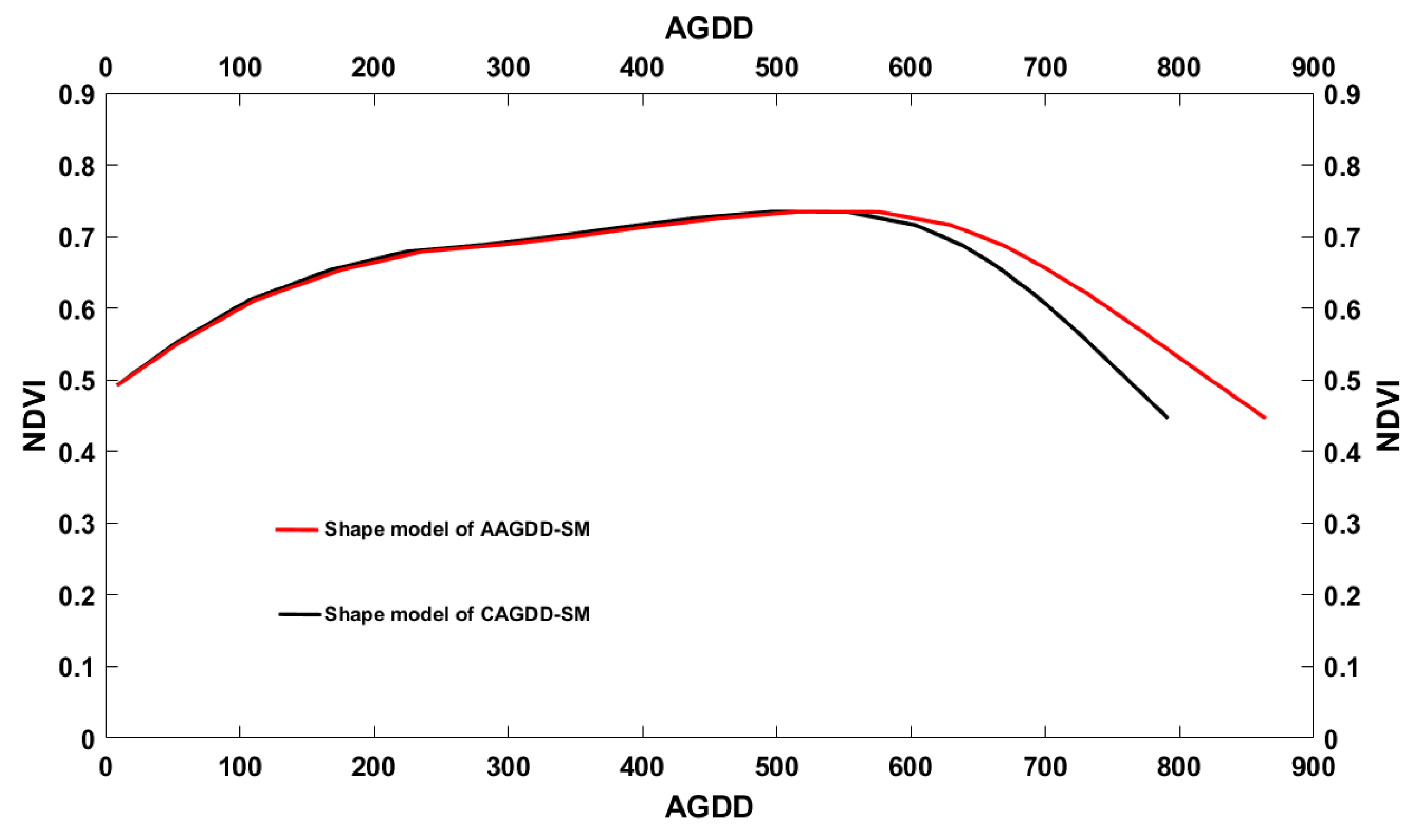
Finally, the AGDD value for day k can be calculated by accumulating the GDD values, and it was further used to replace the calendar day in the shape model as the independent variable, to better reflect the correlation between the shape model and the development of the crop, thereby obtaining more accurate information about the phenological phases. The generated shape models with the proposed continuous AGDD and the average AGDD (namely CAGDD-SM and AAGDD-SM) are shown in Figure 5.
Furthermore, the newly proposed CAGDD-SM method was used to match the growth curve of each year, and the optimal matching parameters of the corresponding year were obtained. These matching parameters can therefore be used to estimate the AGDD value for each phenological period of a certain year, as Equation (8) shows:
A G D D e s t = x s c a l e × ( A G D D X 0 s + t s h i f t )
in which A G D D X 0 S is obtained by averaging the AGDD values corresponding to the ground observation dates of each phenological period in multiple years. Then, we can estimate the phenology in calendar date from AGDD. The specific conversion between them is described in Section 3.1. With the estimated phenological periods of different years, the accuracies of different phenological extraction methods for the years 2014–2018 (excluding 2015) can be calculated, as Equation (9) shows:
R M S E = [ 1 4 i = 1 , 2 , 3 , 4 ( X 0 i X e s t i ) 2 ] 1 2
where i represents the number of observation years, X 0 i refers to the actual observation value of the phenological period, and X e s t i refers to the predicted value of the phenology.

2.2.3. Supplement of Continuous Accumulated Growing Degree Days Model

According to the sine method, the daily temperature curve was fitted. Due to the influence of some abnormal weather, it seems that the fitted curve was not very reasonable, as shown in Figure S5a. Therefore, when fitting the temperature curve, it should be as close as possible to the real temperature curve. Then, according to the rule of calculating the growing degree day by the sine method, the integral of the temperature curve under this fitting method was calculated in combination with the cardinal temperatures, which was the growing degree day of this method. This fitting method was called the curve fitting method. As shown in Figure S5c,d, the curve fitting method was the sum of three sine functions, which was the closest fitting to the original curve.
In addition, because the daily hourly temperature in these years was known, the hourly GDD can be calculated by combining the cardinal temperatures, and the GDD of the day can be obtained by adding up the hourly value for 24 h and dividing it by 24 (Equation (10)). This method was called the time interval control method.
G D D = ( j = 1 24 H G D D j ) / 24
in which HGDD represents the hourly GDD of the day.

3. Results and Discussions

3.1. Phenological Extraction

In this experimental part, the observed phenological periods of years 2014–2018 (excluding 2015) were used to generate the averaging phenological parameters of the shape model, and also to evaluate different phenological extraction methods by matching their growth curves with the shape model to obtain the estimated phenological periods. In this way, the observed phenological periods of the years 2014–2018 (excluding 2015) can be used as the ground truth. Two shape model-based methods, CD-SM and AAGDD-SM were introduced for comparison with the proposed CAGDD-SM method. The generated average phenological periods, X 0 s , and their corresponding A G D D X 0 s values for the CD-SM and CAGDD-SM methods are listed in Table 2, respectively. Given the obtained optimal matching parameters for the different shape models with the annual growth curve, the estimated phenological periods of CD-SM can be obtained directly with Equation (4), while that of CAGDD-SM and AAGDD-SM can be obtained, as Table 3 and Table 4 illustrates.
Based on the GDD calculation, the relationship between the calendar day of different phenological dates and its corresponding AGDD value can be built, as shown in Table 3 and Table 4. For example, the estimated AGDD value of the reviving phase of the year 2018 using the shape model is 133.18, and it is calculated from the daily 24-h temperatures that this AGDD value is between days 11–12. Therefore, the estimated calendar day of the Reviving phase for the year 2018 can be determined as the 11th day.
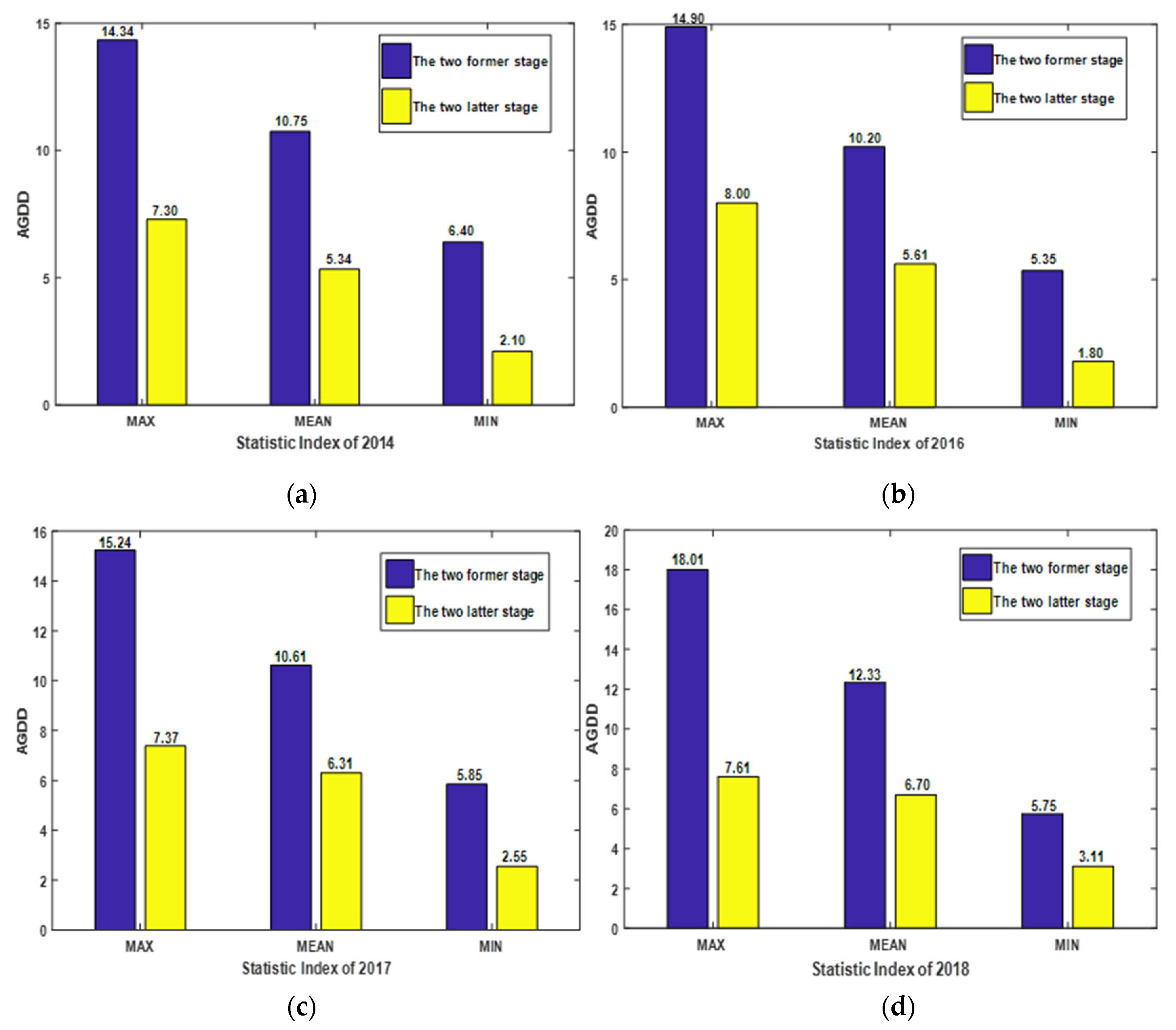
It can be seen from Table 5 that the total accuracy error of method CAGDD-SM (RMSE = 23.64) is better than that of method AAGDD-SM (RMSE = 25.31) and CD-SM (RMSE = 27.87); this has obvious advantages in the reviving and tillering phases. The error of tillering obtained by CAGDD-SM is 2.27 times smaller than that obtained by CD-SM. In any year, the maximum value, minimum value and average value of daily growing degree day in the first two phenological periods were much higher than those in the latter two phenological periods, especially in 2016, where the minimum value of growing degree day in the first two phenological periods was three times that in the latter two phenological periods (Figure 6). In other words, the difference in AGDD obtained by observation between two adjacent days is much larger in the first two phenological periods than in the last two phenological periods. Because the GDD of the last two phenological phases is smaller than that of the first two phenological phases, it leads to the greater floating range of the predicted calendar day after the conversion of the last two phenological periods. Therefore, the estimation errors of the heading date and anthesis date will be relatively high. By observing the daily growing degree day in each phenological period, it was found that the daily growing degree day in the vegetative growth period was generally high, but the growing degree day in the reproductive growth period was relatively low. Therefore, when the estimated error of accumulated growing degree days was the same, the error of calendar time after conversion in the vegetative growth period will be smaller.
It can be seen from Figure 7a that the error range of the phenological period estimated by the shape model based on calendar time was 0–10 days, and the error was about 10 days from the reviving period to the anthesis period. Compared with the former, most of the estimation errors of each phenological period in Figure 7b tended to be closer to the centerline, that is, the errors were smaller. The result shown in Figure 7b is illustrated in Figure 6, and it is also the conversion error caused by the difference between the GDD in different stages. Compared with the other two phenological periods, the daily GDD of the heading and anthesis are smaller, so when it is converted from AGDD to the calendar date, its floating days are larger, resulting in larger errors. Therefore, in the last two phenological periods in Figure 7b, there are some cases with large deviation days.

3.2. Verification of Rationality of Extracting Phenological Period by CAGDD-SM Method

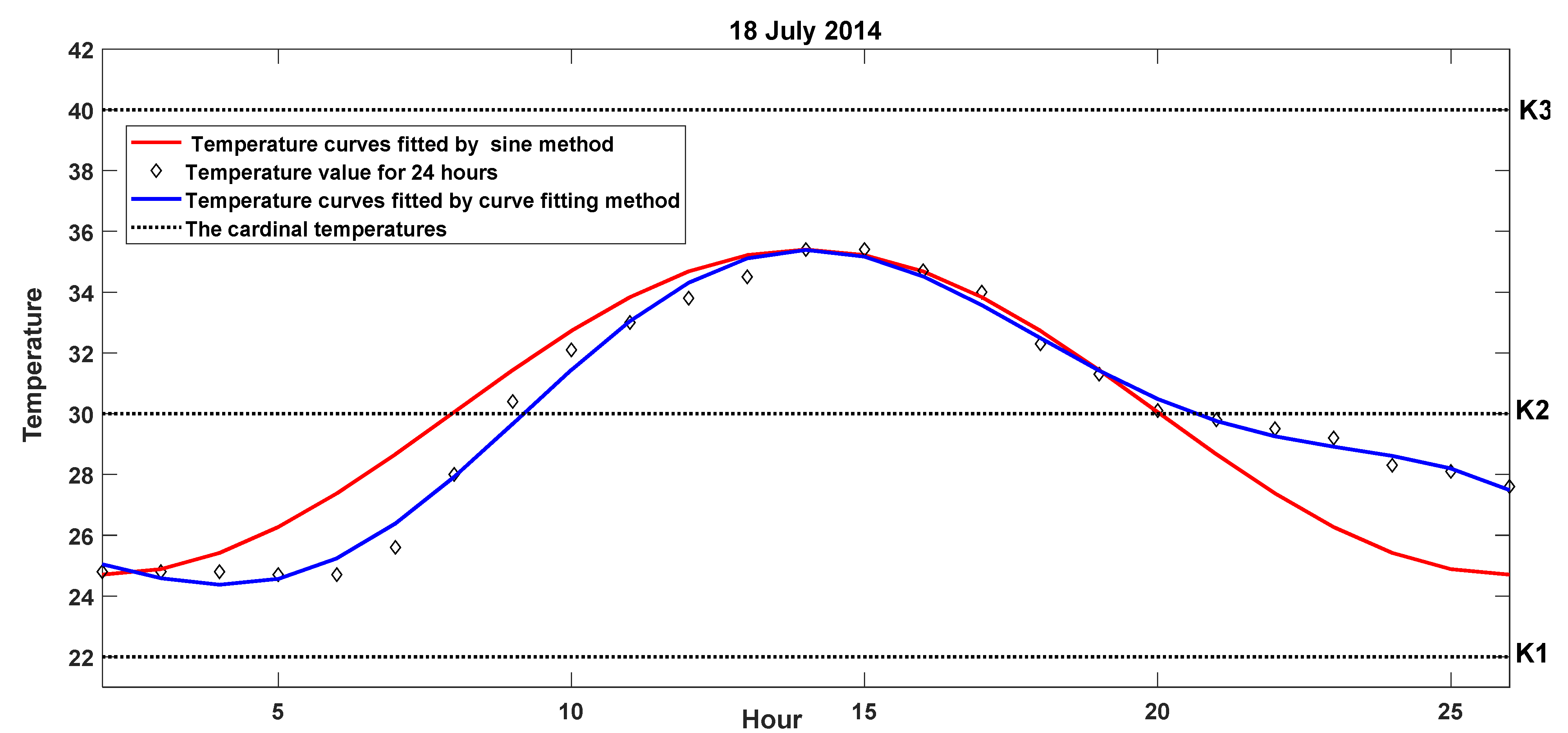
In Figure 8, the red curve is the temperature curve fitted by the CAGDD-SM method, the blue curve is the temperature curve fitted by the curve fitting method (CFAGDD-SM), and the three horizontal lines refer to the cardinal temperatures.
It can be seen from Figure 8 that for some abnormal temperature curves, the curve fitted by the sine method was not as close to the original temperature curve as the curve fitting method. Therefore, in this paper, the curve fitting method (CFAGDD-SM) and time interval method (HAGDD-SM) were used to calculate the accumulated growing degree days, and the other steps were the same as the CAGDD-SM, and the phenological errors of these two methods were obtained (Table 6).
It can be seen from Table 6 that the effect of CAGDD-SM was the best, which was better than CFAGDD-SM. This was contrary to the expected result of CFAGDD-SM. The reason was that the law of accumulated growing degree days assumes that the temperature during the day and at night has the same effect on crop development, which was unreasonable. According to the daily hourly temperature data, the lowest temperature is at around 5:00 to 6:00 in the morning and the highest temperature is at around 2:00 to 4:00 in the afternoon. It can be seen from Figure 8 that the sinusoidal method enlarged the weight of the daytime and weakened the influence of night on the GDD (it was assumed that daytime is 6–18 o’clock). Therefore, CAGDD-SM was more effective than CFAGDD-SM. The date in Figure 8 was just an example. Any date can be used to explain that CAGDD-SM is better than CFAGDD-SM. For example, the two unusual date curves in Figure S5 can also be explained in this way. Similarly, this explains why HAGDD-SM was less effective than AAGDD-SM, because AAGDD-SM calculated GDD by the lowest and highest average values, and the average temperature was in the daytime range, which enlarged the daytime weight. While HAGDD-SM was calculated based on the same influence of day and night on GDD. Therefore, CAGDD-SM had the best effect.

4. Conclusions

Temperature is the most important factor, which is used to extract phenology instead of calendar day as a dependent variable. As for the index of temperature-accumulated growing degree days, it is assumed that the growth rate of crops is positively correlated with temperature, and only when the active growing degree day exceeds the minimum temperature of crops will the crops begin to grow. The active growing degree day defined by accumulated temperature theory is the average value of daily minimum temperature and maximum temperature, which ignores the difference of daily temperature and misses the growing degree day for some days; although the average temperature is lower than the minimum temperature of crops, there are some moments when the temperature is higher than the minimum temperature of crops. Therefore, the sine method is used to calculate the growing degree day every day, which can avoid the above situations.
The daily GDD can be calculated more accurately using the sine method, and the accumulated growing degree days calculated using this method are combined with the shape model (CAGDD-SM). Compared with the accumulated growing degree days calculated using the traditional and common average temperature method, the estimation errors of each phenological period extracted by CAGDD-SM are better than that of the AAGDD-SM method, and the overall error is also better than that of the shape model with calendar time as the dependent variable. CAGDD-SM reduces the situation that some AGDD in AAGDD-SM are calculated as 0 but plants are still growing, so the prediction of the phenology of the former is improved compared to that of the latter. Although the precision of the heading date and anthesis date extracted by CAGDD-SM were worse than that without temperature, this phenomenon appears not only in this experiment; Zhou (2020) also showed that the precision of the reproductive growth period extracted by AAGDD-SM was worse than that of the vegetative growth period.
To verify the rationality of the CAGDD-SM method, this paper also uses the HAGDD-SM method and the CFAGDD-SM method to compare with CAGDD-SM, and the results show that the CAGDD-SM method is still the best. In addition, different from previous studies, the farmland in this study area is an area of ordinary cultivated land, which has neither advanced irrigation equipment nor unified and strict planting density planning. Agricultural producers rely on their own experience to plant and irrigate this cultivated land. Therefore, the research in this paper has more practical significance and achieved good results. Although the method in this paper needs daily hourly temperature data, which may be more difficult to obtain than the average temperature method, the method provided in this paper is based on a more accurate and reasonable AGDD calculation method to predict, and the obtained phenological period is more accurate. For example, for a specific date, the average temperature is less than K1. According to the calculation of the AAGDD-SM, the GDD on that day is 0, but the plants have not stopped growing. CAGDD-SM can greatly reduce these situations. Taking early rice as an example, the transplanting period of early rice usually starts from the end of April to the beginning of May, and the early rice matures at the end of July. The daily temperature difference during this period is not as obvious as that in winter, so the advantages of method A are not so prominent. The emphasis of this paper is to provide a more accurate phenological prediction method.
Therefore, the research in this paper has great potential in crop phenology estimation at a regional scale and provides a lot of useful information for agricultural production. Accurate phenological information can help to make a reasonable agricultural production plan, and facilitate work such as crop cultivation, pest control, and crop yield estimation. The research in this paper has the potential to be applied to the phenological period estimation of other crops, such as cotton, soybean, and corn. Future work is based on the existing research, considering the difference of accumulated growing degree days between day and night, to further improve the estimation of crop phenological period. In addition, the emphasis of this paper is to consider more reasonable and accurate temperatures based on SM, and more factors can be considered in the future, such as the influence of water, soil and different vegetation indexes. This paper adopts a more reasonable method to calculate AGDD and combines it with the shape model to get a more accurate estimation of the phenological period. Finally, the rationality of this proposed method (CAGDD-SM) is also verified and can provide useful help for agricultural production planning.

Supplementary Materials

The following supporting information can be downloaded at: https://www.mdpi.com/article/10.3390/rs14215337/s1, Figure S1: The fitted growth curve from MODIS NDVI data for year i; Figure S2: Matching of shape model with growth curve; Figure S3: An example of 24-h temperature fitting; Figure S4: Eight cases to calculate the GDD value. (A,B) refer to the case where the daily maximum temperature is greater than K1 and less than K2. (C–E) refer to the case where the daily maximum temperature is greater than K2 and less than K3. (F–H) refer to the case where the daily maximum temperature is greater than K3; Figure S5: The temperature curves fitted by the sine method and the curve fitting method. (a,b) are temperature curves fitted by the sine method; (c,d) are temperature curves fitted by curve fitting method.

Author Contributions

S.L.: Methodology, validation, writing—original draft; X.X.: Conceptualization, methodology, writing—reviewing and editing, supervision; H.X.: Formal analysis, supervision, writing—reviewing and editing; P.C.: Supervision; C.W.: Writing—reviewing and editing, formal analysis; Y.J.: Visualization; X.T.: Funding acquisition, project administration; C.X.: Data curation. All authors have read and agreed to the published version of the manuscript.

Funding

This research was partly supported by the National Key Research & Development Program of China under Grant 2018YFB0505400, the National Natural Science Foundation of China under Grant 41971299 and 42221002, the Shanghai Municipal Science and Technology Major Project under Grant 2021SHZDZX0100, the Shanghai Municipal Commission of Science and Technology Project under Grant 19511132101 and the Fundamental Research Funds for the Central Universities.

Data Availability Statement

Ground observation phenological information and daily hourly temperature data are not available. Data were obtained from the Leping city Meteorological Bureau but are confidential. Remote sensing data can be accessed and downloaded from the United States Geological Survey (USGS). This data can be found here: https://ladsweb.modaps.eosdis.nasa.gov/search (accessed on 1 July 2022).

Acknowledgments

We want to thank the Leping city Meteorological Bureau for allowing us to use the data in this study.

Conflicts of Interest

The authors declare no conflict of interest.

References

  1. Körner, C.; Basler, D. Phenology Under Global Warming. Science 2010, 327, 1461–1462. [Google Scholar] [CrossRef] [PubMed]
  2. Zwart, S.J.; Bastiaanssen, W.G.M. Review of measured crop water productivity values for irrigated wheat, rice, cotton and maize. Agric. Water Manag. 2004, 69, 115–133. [Google Scholar] [CrossRef]
  3. Pimstein, A.; Eitel, J.; Long, D.; Mufradi, I.; Karnieli, A.; Bonfil, D. A spectral index to monitor the head-emergence of wheat in semi-arid conditions. Field Crop. Res. 2009, 111, 218–225. [Google Scholar] [CrossRef] [Green Version]
  4. Xiao, D.P.; Tao, F.L.; Liu, Y.J.; Shi, W.J.; Wang, M.; Liu, F.S.; Zhang, S.A.; Zhu, Z. Observed changes in winter wheat phenology in the North China Plain for 1981–2009. Int. J. Biometeorol. 2013, 57, 275–285. [Google Scholar] [CrossRef]
  5. Akhtar, F.; Awan, U.K.; Tischbein, B.; Liaqat, U.W. A phenology based geo-informatics approach to map land use and land cover (2003–2013) by spatial segregation of large heterogenic river basins. Appl. Geogr. 2010, 88, 48–61. [Google Scholar] [CrossRef]
  6. Liu, L.L.; Zhang, X.Y.; Yu, Y.Y.; Gao, F.; Yang, Z.W. Real-Time Monitoring of Crop Phenology in the Midwestern United States Using VIIRS Observations. Remote Sens. 2018, 10, 1540. [Google Scholar] [CrossRef] [Green Version]
  7. Rembold, F.; Meroni, M.; Urbano, F.; Csak, G.; Kerdiles, H.; Perez-Hoyos, A.; Lemoine, G.; Leo, O.; Negre, T. ASAP: A new global early warning system to detect anomaly hot spots of agricultural production for food security analysis. Agric. Syst. 2019, 168, 247–257. [Google Scholar] [CrossRef]
  8. Skawsang, S.; Nagai, M.; Tripathi, N.K.; Soni, P. Predicting Rice Pest Population Occurrence with Satellite-Derived Crop Phenology, Ground Meteorological Observation, and Machine Learning: A Case Study for the Central Plain of Thailand. Appl. Sci. 2019, 9, 4846. [Google Scholar] [CrossRef] [Green Version]
  9. Funk, C.; Budde, M.E. Phenologically-tuned MODIS NDVI-based production anomaly estimates for Zimbabwe. Remote Sens. Environ. 2009, 113, 115–125. [Google Scholar] [CrossRef]
  10. Bolton, D.K.; Friedl, M.A. Forecasting crop yield using remotely sensed vegetation indices and crop phenology metrics. Agric. For. Meteorol. 2013, 173, 74–84. [Google Scholar] [CrossRef]
  11. Sakamoto, T.; Gitelson, A.A.; Arkebauer, T.J. MODIS-based corn grain yield estimation model incorporating crop phenology information. Remote Sens. Environ. 2013, 131, 215–231. [Google Scholar] [CrossRef]
  12. Magney, T.; Eitel, J.; Huggins, D.; Vierling, L. Proximal NDVI derived phenology improves in-season predictions of wheat quantity and quality. Agric. For. Meteorol. 2016, 217, 46–60. [Google Scholar] [CrossRef]
  13. Gao, F.; Anderson, M.C.; Zhang, X.Y.; Yang, Z.W.; Alfieri, J.G.; Kustas, W.P.; Mueller, R.; Johnson, D.M.; Prueger, J.H. Toward mapping crop progress at field scales through fusion of Landsat and MODIS imagery. Remote Sens. Environ. 2017, 188, 9–25. [Google Scholar] [CrossRef] [Green Version]
  14. Kang, Y.H.; Özdoğan, M. Field-level crop yield mapping with Landsat using a hierarchical data assimilation approach. Remote Sens. Environ. 2019, 228, 144–163. [Google Scholar] [CrossRef]
  15. Mateo-Sanchis, A.; Piles, M.; Muñoz-Marí, J.; Adsuara, J.E.; Pérez-Suay, A. Synergistic integration of optical and microwave satellite data for crop yield estimation. Remote Sens. Environ. 2019, 234, 111460. [Google Scholar] [CrossRef]
  16. Zeng, L.L.; Wardlow, B.; Xiang, D.; Hu, S.; Li, D. A review of vegetation phenological metrics extraction using time-series, multispectral satellite data. Remote Sens. Environ. 2020, 237, 111511. [Google Scholar] [CrossRef]
  17. Mayer, A. Phenology and citizen science. Bioscience 2010, 60, 172–175. [Google Scholar] [CrossRef] [Green Version]
  18. Dai, J.; Xu, Y.; Wang, H.; Alatalo, J.; Tao, Z. Variations in the temperature sensitivity of spring leaf phenology from 1978 to 2014 in Mudanjiang, China. Int. J. Biometeorol. 2017, 63, 569–577. [Google Scholar] [CrossRef]
  19. Yan, D.; Zhang, X.Y.; Nagai, S.; Yu, Y.Y.; Akitsu, T.; Nasahara, K.N.; Ide, R.; Maeda, T. Evaluating land surface phenology from the Advanced Himawari Imager using observations from MODIS and the Phenological Eyes Network. Int. J. Appl. Earth Obs. 2019, 79, 71–83. [Google Scholar] [CrossRef]
  20. Vrieling, A.; Meroni, M.; Darvishzadeh, R.; Skidmore, A.; Wang, T.; Zurita-Milla, R.; Oosterbeek, K.; O’Connor, B.; Paganini, M. Vegetation phenology from Sentinel-2 and field cameras for a Dutch barrier island. Remote Sens. Environ. 2018, 215, 517–529. [Google Scholar] [CrossRef]
  21. Berra, E.F.; Gaulton, R.; Barr, S. Assessing spring phenology of a temperate woodland: A multiscale comparison of ground, unmanned aerial vehicle and Landsat satellite observations. Remote Sens. Environ. 2019, 223, 229–242. [Google Scholar] [CrossRef]
  22. Brown, M.; de Beurs, K.; Marshall, M. Global phenological response to climate change in crop areas using satellite remote sensing of vegetation, humidity and temperature over 26 years. Remote Sens. Environ. 2012, 126, 174–183. [Google Scholar] [CrossRef]
  23. Atzberger, C. Advances in Remote Sensing of Agriculture: Context Description, Existing Operational Monitoring Systems and Major Information Needs. Remote Sens. 2013, 5, 949–981. [Google Scholar] [CrossRef] [Green Version]
  24. Chen, F.X.; Liu, Z.J.; Zhong, H.M.; Wang, S.S. Exploring the Applicability and Scaling Effects of Satellite-Observed Spring and Autumn Phenology in Complex Terrain Regions Using Four Different Spatial Resolution Products. Remote Sens. 2021, 13, 4582. [Google Scholar] [CrossRef]
  25. Babcock, C.; Finley, A.O.; Looker, N. A Bayesian model to estimate land surface phenology parameters with harmonized Landsat 8 and Sentinel-2 images. Remote Sens. Environ. 2021, 261, 112471. [Google Scholar] [CrossRef]
  26. Ishigooka, Y.; Kuwagata, T.; Goto, S.; Toritani, H.; Ohno, H.; Urano, S. Modeling of continental-scale crop water requirement and available water resources. Paddy Water Environ. 2008, 6, 55–71. [Google Scholar] [CrossRef]
  27. Zhang, X.; Goldberg, M.D. Monitoring fall foliage coloration dynamics using time-series satellite data. Remote Sens. Environ. 2011, 115, 382–391. [Google Scholar] [CrossRef]
  28. Kobayashi, H.; Yunus, A.P.; Nagai, S.; Sugiura, K.; Kim, Y.; Dam, B.V.; Nagano, H.; Zona, D.; Harazono, Y.; Bret-Harte, M.S. Latitudinal gradient of spruce forest understory and tundra phenology in Alaska as observed from satellite and ground-based data. Remote Sens. Environ. 2016, 177, 160–170. [Google Scholar] [CrossRef] [Green Version]
  29. Reed, B.C.; Brown, J.F.; VanderZee, D.; Loveland, T.R.; Merchant, J.W.; Ohlen, D.O. Measuring phenological variability from satellite imagery. J. Veg Sci. 1994, 5, 703–714. [Google Scholar] [CrossRef]
  30. Zhang, X.; Friedl, M.; Schaaf, C.; Strahler, A.; Hodges, J.; Gao, F. Monitoring vegetation phenology using MODIS time-series data. Remote Sens. Environ. 2003, 84, 471–475. [Google Scholar] [CrossRef]
  31. Tateishi, R.; Ebata, M. Analysis of phenological change patterns using 1982–2000 advanced very high resolution radiometer (AVHRR) data. Int. J. Remote Sens. 2004, 25, 2287–2300. [Google Scholar] [CrossRef]
  32. Sakamoto, T. Refined shape model fitting methods for detecting various types of phenological information on major U.S. crops. ISPRS J. Photogramm. 2018, 138, 176–192. [Google Scholar] [CrossRef]
  33. Liao, C.H.; Wang, J.F.; Dong, T.F.; Shang, J.L.; Liu, J.G.; Song, Y. Using spatio-temporal fusion of Landsat-8 and MODIS data to derive phenology, biomass and yield estimates for corn and soybean. Sci. Total Environ. 2019, 650, 1707–1721. [Google Scholar] [CrossRef] [PubMed]
  34. White, M.A.; Thornton, P.E.; Running, S.W. A continental phenology model for monitoring vegetation responses to interannual climatic variability. Glob. Biogeochem. Cycles. 1997, 11, 217–234. [Google Scholar] [CrossRef]
  35. White, K.; Pontius, J.; Schaberg, P. Remote sensing of spring phenology in northeastern forests: A comparison of methods, field metrics and sources of uncertainty. Remote Sens. Environ. 2014, 148, 97–107. [Google Scholar] [CrossRef]
  36. Mobasheri, M.R.; Chahardoli, M.; Farajzadeh, M. Introducing PASAVI and PANDVI methods for sugarcane physiological date estimation, using ASTER images. J. Agric. Sci. Technol. 2010, 12, 309–320. [Google Scholar]
  37. Moulin, S.; Kergoat, L.; Viovy, N.; Dedieu, G. Global-scale assessment of vegetation phenology using NOAA/AVHRR satellite measurements. J. Clim. 1997, 10, 1154–1170. [Google Scholar] [CrossRef]
  38. Sakamoto, T.; Wardlow, B.; Gitelson, A. A Two-Step Filtering approach for detecting maize and soybean phenology with time-series MODIS data. Remote Sens. Environ. 2010, 114, 2146–2159. [Google Scholar] [CrossRef]
  39. Xiao, J.; Li, N.; Jiang, H.F. Calculation and Stability of Accumulated Temperatures in the Growing Season of Winter wheat. J. Meteor. Res. Appl. 2010, 31, 65–67. [Google Scholar]
  40. Jin, Y.; Wong, K.W.; Wu, Z.D.; Qi, D.B.; Wang, R.; Han, F.; Wu, W.F. Relationship between accumulated temperature and quality of paddy. Int. J. Food Prop. 2019, 22, 19–33. [Google Scholar] [CrossRef] [Green Version]
  41. Chen, T.; Huang, Q.; Gao, D.; Huang, Z.; Zheng, Y.; Li, Y. Accumulated Temperature as an Indicator to Predict the Stabilizing Process in Sewage Sludge Composting. Acta Ecol. Sin. 2002, 22, 911–915. [Google Scholar]
  42. Zeng, L.L.; Wardlow, B.; Li, D. A hybrid approach for detecting corn and soybean phenology with time-series MODIS data. Remote Sens. Environ. 2016, 181, 237–250. [Google Scholar] [CrossRef]
  43. Zhou, M.; Ma, X.; Wang, K.; Cheng, T.; Tian, Y.; Wang, J.; Yao, X.; Zhu, Y. Detection of phenology using an improved shape model on time-series vegetation index in wheat. Comput. Electron. Agric. 2020, 173, 105398. [Google Scholar] [CrossRef]
  44. Watanabe, N. An Improved Method for Computing Heat Accumulation from Daily Maximum and Minimum Temperatures. Appl. Entomol. Zool. 1978, 13, 44–46. [Google Scholar] [CrossRef] [Green Version]
  45. Myneni, R.B.; Hall, F.G.; Sellers, P.J.; Marshak, A.L. The Interpretation of Spectral Vegetation Indexes. IEEE Trans. Geosci. Remote Sens. 1995, 33, 481–486. [Google Scholar] [CrossRef]
  46. dela Torre, D.M.G.; Gao, J.; Macinnis-Ng, C. Remote sensing-based estimation of rice yields using various models: A critical review. Geo Spat. Inf. Sci. 2021, 24, 580–603. [Google Scholar] [CrossRef]
  47. Yang, G.; Huang, K.; Sun, W.W.; Meng, X.C.; Mao, D.H.; Ge, Y. Enhanced mangrove vegetation index based on hyperspectral images for mapping mangrove. ISPRS J. Photogramm. 2022, 189, 236–254. [Google Scholar] [CrossRef]
  48. Lemos, H.D.; Verstraete, M.M.; Scholes, M. Parametric Models to Characterize the Phenology of the Lowveld Savanna at Skukuza, South Africa. Remote Sens. 2020, 12, 3927. [Google Scholar] [CrossRef]
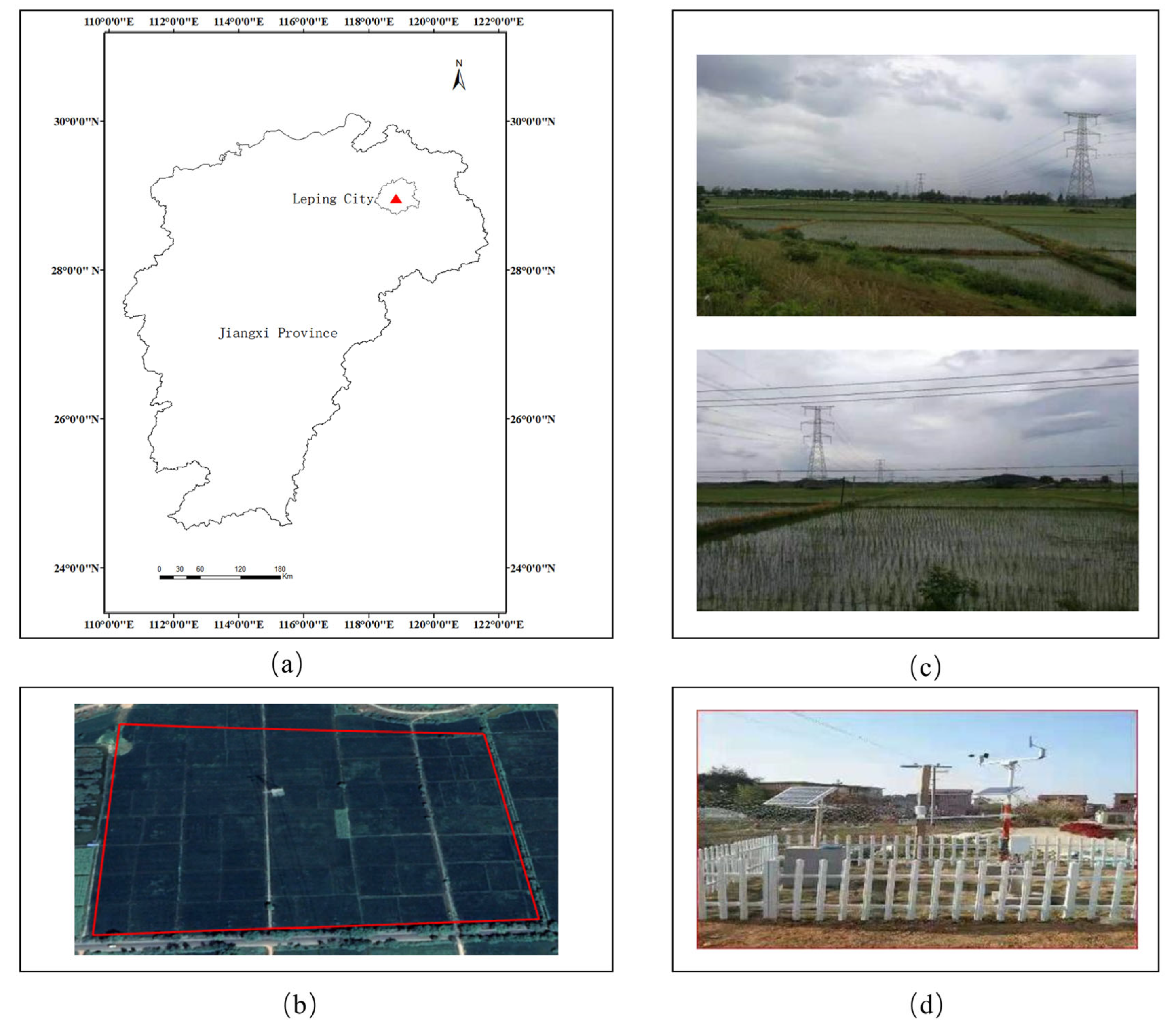
Figure 1. Study area. (a) Location. (b) Google Earth image. (c) Field survey images. (d) Phenological observation stations.
Remotesensing 14 05337 g001
Figure 2. NDVI images generated from MODIS products, the red ROI refers to the corresponding study area. (a) Image of 30 April 2014, which indicates the smallest NDVI value in the growing period of that year. (b) Image of 8 July 2014, which indicates the largest NDVI value in the growing period of that year.
Remotesensing 14 05337 g002
Figure 3. Flowchart of the proposed CAGDD-SM method.
Remotesensing 14 05337 g003
Figure 4. Shape model of early rice based on calendar day.
Remotesensing 14 05337 g004
Figure 5. Shape models of AAGDD-SM and CAGDD-SM.
Remotesensing 14 05337 g005
Figure 6. Comparison of statistical indicators of the first two phenological periods and the last two phenological periods of each year. (ad) indicate the statistical indicators of each year. The blue bars indicate the period between the reviving and tillering stages, while the yellow bars indicate the period between the heading and anthesis stages.
Remotesensing 14 05337 g006
Figure 7. Assessment of phenology dates between the ground-based observations and the estimation derived from the CD-SM and CAGDD-SM. (a) CD-SM. (b) CAGDD-SM.
Remotesensing 14 05337 g007
Figure 8. Comparison of temperature curves fitted by the CAGDD-SM method and the CFAGDD-SM method.
Remotesensing 14 05337 g008
Table 1. The three-cardinal temperatures of the early rice.
Phenology StageK1 (°C)K2 (°C)K3 (°C)
Reviving123242
Tillering153242
Heading223040
Anthesis223040
Table 2. The predefined A G D D X 0 S and X 0 s of different shape models for early rice.
Phenology Stage X 0 s / d A G D D X 0 s / ° C
Reviving765.68
Tillering28305.38
Heading58622.33
Anthesis61634.84
Table 3. The estimated accumulated growing degree days in 2018.
Year 2018RevivingTilleringHeadingAnthesis
The estimated AGDD133.18336.92606.33616.97
Table 4. AGDD calculated from daily 24-h temperatures of the year 2018.
Year 2018Day 1Day 2...Day 9Day 10Day 11Day 12
AGDD value11.1521.65...99.15112.15126.80143.30
Table 5. Precisions of different phenological extraction methods.
Phenology StageRMSE (Day)
CD-SMAAGDD-SMCAGDD-SM
Reviving6.804.124.15
Tillering6.643.352.92
Heading7.208.347.78
Anthesis7.239.508.79
All27.8725.3123.64
Table 6. Estimation errors of CAGDD-SM, CFAGDD-SM and HAGDD-SM.
Phenology StageRMSE (Day)
CAGDD-SMCFAGDD-SMHAGDD-SM
Reviving4.154.534.15
Tillering2.923.353.35
Heading7.788.678.67
Anthesis8.799.229.66
All23.6425.7725.83
Publisher’s Note: MDPI stays neutral with regard to jurisdictional claims in published maps and institutional affiliations.