Article

Understanding Water Level Changes in the Great Lakes by an ICA-Based Merging of Multi-Mission Altimetry Measurements

1
College of Resource Environment and Tourism, Hubei University of Arts and Science, Xiangyang 441053, China
2
Division of Geodetic Science, School of Earth Sciences, Ohio State University, Columbus, OH 43210, USA
3
Department of Planning, Aalborg University, 9220 Aalborg, Denmark
4
School of Geospatial Engineering and Science, Sun Yat-Sen University, Zhuhai 519082, China
5
School of Geomatics Science and Technology, Nanjing Tech University, Nanjing 211800, China
6
State Key Laboratory of Geodesy and Earth’s Dynamics, Innovation Academy for Precision Measurement Science and Technology, Chinese Academy of Sciences, Wuhan 430071, China
7
School of Geographic Information and Tourism, Chuzhou University, Chuzhou 239099, China
*
Author to whom correspondence should be addressed.
Remote Sens. 2022, 14(20), 5194; https://doi.org/10.3390/rs14205194
Submission received: 13 September 2022 / Revised: 12 October 2022 / Accepted: 14 October 2022 / Published: 17 October 2022
(This article belongs to the Special Issue Carbon, Water and Climate Monitoring Using Space Geodesy Observations)

Abstract

:
Accurately monitoring spatio-temporal changes in lake water levels is important for studying the impacts of climate change on freshwater resources, and for predicting natural hazards. In this study, we applied multi-mission radar satellite altimetry data from the Laurentian Great Lakes, North America to optimally reconstruct multi-decadal lake-wide spatio-temporal changes of water level. We used the results to study physical processes such as teleconnections of El Niño and southern oscillation (ENSO) episodes over approximately the past three-and-a-half decades (1985–2018). First, we assessed three reconstruction methods, namely the standard empirical orthogonal function (EOF), complex EOF (CEOF), and complex independent component analysis (CICA), to model the lake-wide changes of water level. The performance of these techniques was evaluated using in-situ gauge data, after correcting the Glacial Isostatic Adjustment (GIA) process using a contemporary GIA forward model. While altimeter-measured water level was much less affected by GIA, the averaged gauge-measured water level was found to have increased up to 14 cm over the three decades. Our results indicate that the CICA-reconstructed 35-year lake level was more accurate than the other two techniques. The correlation coefficients between the CICA reconstruction and the in situ water-level data were 0.96, 0.99, 0.97, 0.97, and 0.95, for Lake Superior, Lake Michigan, Lake Huron, Lake Erie, and Lake Ontario, respectively; ~7% higher than the original altimetry data. The root mean squares of errors (RMSE) were 6.07 cm, 4.89 cm, 9.27 cm, 7.71 cm, and 9.88 cm, respectively, for each of the lakes, and ~44% less than differencing with the original altimetry data. Furthermore, the CICA results indicated that the water-level changes in the Great Lakes were significantly correlated with ENSO, with correlation coefficients of 0.5–0.8. The lake levels were ~25 cm higher (~30 cm lower) than normal during EI Niño (La Niña) events.

Graphical Abstract

1. Introduction

The Great Lakes of North America are the largest group of freshwater lakes on Earth by area, and provide drinking water, food, and recreation to 40 million people, and billions of dollars in economic benefits to the region [1]. Lake-level changes are considered directly representative of water resources, and are sensitive to climate change including precipitation increases, ice cover decline, water temperature rises, and global-scale El Niño Southern Oscillation (ENSO) [2], along with anthropogenic influences such as drinking water processing, industrial use, and channel dredging [3,4,5]. Quinn found that Great Lakes’ water levels had a well-defined seasonal cycle driven primarily by snowmelt in the spring and summer and lake evaporation in the fall and winter [6]. Burton reported that the coastal marshes of the Great Lakes could be affected by unique fluctuations in water level due to seiche activity in the lakes [7]. According to predictions made by Kayastha et al., by 2040–2049 the average annual water levels of Lake Superior, Michigan–Huron, and Erie are projected to increase by 0.19, 0.44, and 0.28 m, respectively, relative to 2010–2019 [8]. In recent years, the Great Lakes’ water levels have demonstrated more frequent and intensive fluctuation. For example, the lowest measurements on record were taken in 2013 for most of the Great Lakes, i.e., ~30 cm reduction, while Lake Superior and Lake Michigan–Huron contained ~35 cm less water in 2014, and severe flooding happened in 2017 on Lake Ontario, exceeding 40 cm increase in water level [9]. Hence, comprehensive spatio-temporal monitoring of lake-level changes is vitally important in the Great Lakes.
Generally, measurements of lake surface height have mainly relied on satellite altimetry [10,11,12] and in situ water level stations [13,14]. Hwang et al. verified that there were good agreements between the TOPEX/Poseidon altimetry data and gauge results at Bosten Lake (western China) and Lake Huron (North America). Wang et al. presented a robust strategy to estimate the lake level of Ngangzi Co, with an accuracy of ~17 cm for TOPEX/Poseidon and ~10 cm for Jason-1/2/3. Sun et al. constructed a 27-year lake-level time series for Zhari Namco, using the TOPEX/Poseidon-Jason1/2/3 and validating temperature, precipitation, lake area, equivalent water height, and in situ gauge data. The GeoSat data for the Great Lakes were compared to data from water level stations in 1994, and it was found that the root mean squares of errors (RMSE) could be up to 11.1 cm [15]. Jekeli et al. studied the establishment of vertical data with satellite altimetry and water-level gauge data on large lakes, and showed a tilt of about 33 cm in the computed data across the Great Lakes [16]. Kuo et al. estimated vertical crustal motions by combining geocentric sea-level measurements and water-level gauges in the Great Lakes area, the uncertainties were estimated at <0.5 mm/year [17]. Cheng et al. calibrated the surface height of the Great Lakes using Jason-1 and Jason-2, with comparable results to those from the dedicated sites [18]. In a recent study, a multi-mission satellite radar altimetry-based database has been established in the Great Lakes region, using GDR and RADS data from 12 radar altimetry satellites (Geosat, GFO, ERS-1/-2, Envisat, TOPEX/Poseidon, Jason-1/-2/-3, SARAL/Altika, CryoSat-2, Sentinel-3A) covering ~35 years, to improve monitoring and enhance the Great Lakes Operational Forecasting System [19]. Although satellite altimetry can provide measurements of spatial water-level changes across these lakes, there remains limited information due to data gaps and limited coverage from satellite tracks. In situ water level stations provided long-term continuous measures of fluctuations, but are limited to certain locations distributed along the shorelines. The limitations of these two measurement techniques impede comprehensive research of inland hydrology and water resources, including addressing spatial and temporal dynamics of freshwater storage, flood forecasting, and other water resource management applications [20,21].
In most previous studies, statistical reconstruction was implemented based on principal component analysis (PCA), also known as the empirical orthogonal function (EOF) [22,23] technique. This process is known as optimal space–time reconstruction, and has been widely applied in sea-level reconstruction due to its simplicity and operability [24,25,26,27]. However, from the mathematical perspective, the popular PCA/EOF is a second-order and stationary statistical decomposition technique, because by definition it considers the lag-zero auto-covariance of observations to estimate statistically orthogonal eigenvectors known as orthogonal modes [28]. In reality, the time series of water-level fluctuations represents dynamical characteristics that include monotonic trends and inter-annual cyclic variations [29,30]. Therefore, non-stationary techniques such as the complex extension of PCA/EOF, known as CEOF [31], can be considered to better represent the cyclo-stationary properties of the water-level time series [32,33]. Forootan and Kusche argued that geophysical time series usually contain statistical information considerably higher than the second order, provided in the higher-order statistical content of the probability distribution function (PDF), which can be extracted from the observed results [34,35,36]. Thus, the higher-order statistical information is incorporated in the independent component analysis (ICA) method to separate spatial and temporal geophysical time series into statistically independent modes, which are likely to be better correlated with independent physical processes according to the measurements [37,38,39]. Forootan et al. successfully applied this technique for reconstructing global terrestrial water-storage fields. Forootan et al. extended the stationary ICA method to account for cyclo-stationary statistical properties of samples’ time series through the complex ICA (CICA) approach, the performance of which was tested by analyzing various satellite-derived time series [30]. In the current study, we tested how CICA can be helpful to reconstruct surface water level changes in the Great Lakes area, which exhibit considerable fluctuations over different time scales.
The Great Lakes are often referred to as inland seas because of their sea-like characteristics, including rolling waves, sustained winds, strong currents, great depths, and distant horizons [40]. Therefore, the main motivation of this study was to incorporate the merits of satellite altimetry and in situ measurements, borrowed from the sea-level reconstruction, using decomposition-based reconstruction algorithms to obtain spatial and temporal dynamics of water-level changes in the Great Lakes. Before the reconstruction, the glacial isostatic adjustment (GIA) corrections (including radial displacement and geoid changes in the Great Lakes) were applied to ensure data consistency. The CICA and ordinary EOF and CEOF reconstructions were implemented to produce a long-term (April 1985–October 2018) dataset of surface height changes across the Great Lakes. The changes were spatially and temporally dense, and were homogenized with 0.1° × 0.1° and monthly spatio-temporal resolution. The reconstructions were evaluated in terms of correlation coefficients and RMSE, by comparison with the water-level changes reported by in situ stations. We also assessed the interannual water-level fluctuations caused by the El Niño–Southern Oscillation (ENSO) to assess whether the lakes’ surface heights during ENSO events were higher or lower than normal.

2. Data and Methods

2.1. Study Area

The Great Lakes, also called the Laurentian Great Lakes, consist of Lakes Superior, Michigan, Huron, Erie, and Ontario (see Figure 1). They are primarily located in the upper mid-east region of North America and are on the Canada–United States border, ranging from 41°N to 50°N latitude and 75°W to 93°W longitude, with total surface area and total volume up to 244,106 km2 and 22,671 km3, respectively [41].

2.2. Radar Altimetry Data

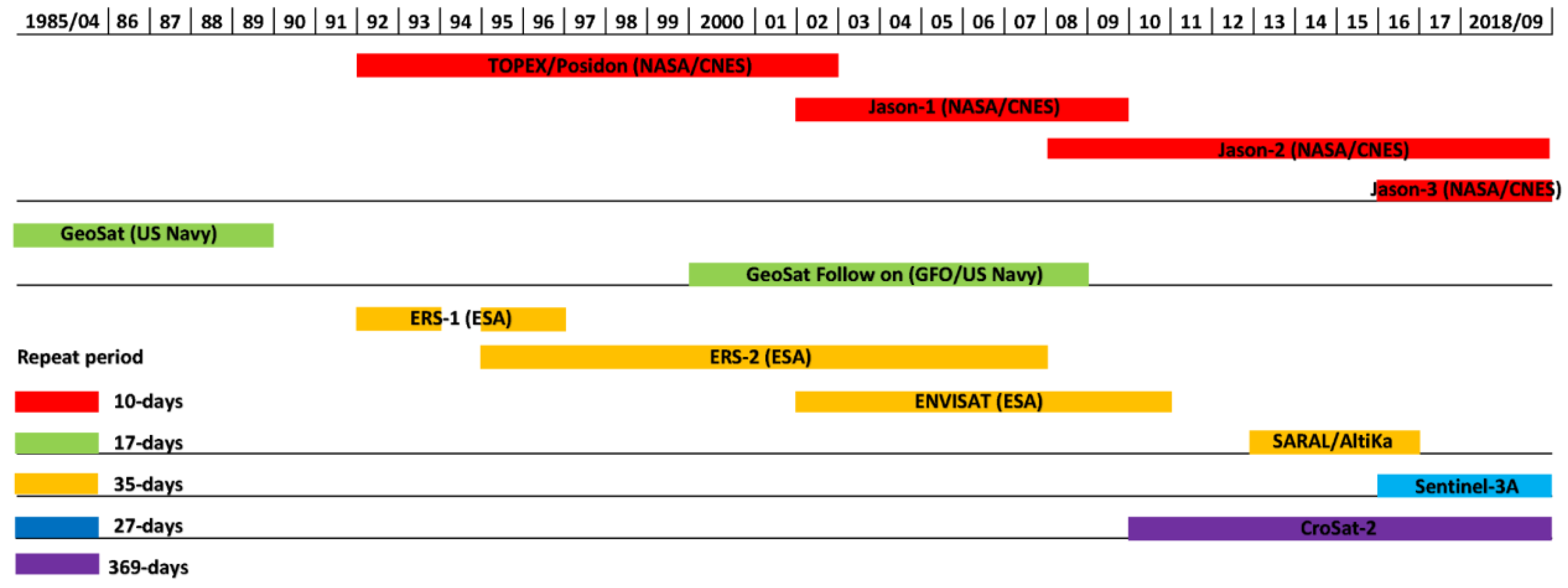
The radar altimetry data used in this study were from the Geophysical Data Records (GDR) and Radar Altimeter Database System (RADS), from April 1985 to September 2018. GDR mainly includes TOPEX/Poseidon (T/P), Jason-1, Jason-2, Jason-3, ERS-1, ERS-2, ENVISAT, and SARAL/AltiKa data products (https://www.aviso.altimetry.fr/en/data/products/sea-surface-height-prodcts/global/gdr-igdr-and-ogdr.html (accessed on 15 December 2020)); RADS mostly covers GEOSAT (GEOdetic SATellite), GEOSAT Follow-on (GFO), Sentinel-3A, and CryoSat-2 data products (http://rads.tudelft.nl/rads/rads.shtml (accessed on 15 December 2020)). The temporal coverage provided by the altimetry data products is indicated in Figure 2.
The primary results from radar altimetry satellites were the ranges, i.e., the distances between the satellite orbit and the water level measured with respect to the reference ellipsoid [42]. In order to compute water level, further processing was applied. First, estimation of surface height anomaly was obtained from Equations (1) and (2), which apply geophysical and atmospheric corrections:
h LSHA = h LSH h geoid = h A ( h R + h C ) h EGM + ε
h c = h i + h wet + h dry + h iono + h se + h pol
where h LSHA is geocentric lake surface height anomaly (LSHA); h LSH and h geoid represent lake surface height (LSH) and the EGM2008 geoid height, respectively; h A , h R , and h C refer to the orbital height above the reference ellipsoid, the altimeter range, and the altimeter range corrections, respectively. The corrections applied to the altimeter range ( h C ) consisted of instrument corrections ( h i ), wet troposphere correction ( h wet ), dry troposphere correction ( h dry ), ionosphere correction ( h iono ), and geophysical corrections of the solid Earth tide ( h se ) and pole tide ( h pol ). The data editing was followed by the standard procedure which included: (1) extracting altimetry measurements within the Great Lakes by utilizing water masks; (2) removing unreasonable and large outliers according to wave-height threshold; (3) separating ice-cover information contaminating the altimetry observations; (4) dealing with apparently false values by applying an alternative median absolute deviation (MAD) method; (5) estimating accurate altimetry measurements by applying Gaussian kernel regression (GKR) to remove outliers. Finally, we obtained the water-level changes from the multi-mission radar altimetry after removing bias between different satellites.

2.3. Water Level Stations

The in situ data from the Great Lakes are among the longest and highest-quality hydro-meteorological datasets in North America, having been collected since 1860. Figure 1a shows the water-level stations maintained by NOAA/NOS/CO-OPS (https://www.glerl.noaa.gov/data/wlevelsl (accessed on 20 December 2018)) and DFO/CHS (http://www.isdm-gdsi.gc.ca/isdm-gdsi/twl-mnel (accessed on 20 December 2018)). At these stations, water levels are recorded at 6-min intervals and archived at hourly, daily, and monthly intervals. In the current study, the lake-wide network average was used for calculating the lakes’ average surface height.

2.4. Glacial Isostatic Adjustment

The Great Lakes formed at the end of the last glacial period, around 14,000 years ago. [1,43]. GIA is the result of the natural rebound of the Earth’s crust following the removal of the weight of the glaciers that covered the region [44,45]. During satellite altimetry, GIA affects the geoid change which is subtracted in Equation (1). Meanwhile, water level stations established on pedestal rocks are also influenced by the radial displacement from GIA. In this study, we used the newly released ICE-6G model to estimate geoid changes and radial displacement (https://www.atmosp.physics.utoronto.ca/~peltier/data.phpl (accessed on 25 December 2018)).

2.5. Multivariate ENSO Index

The El Niño–Southern Oscillation (ENSO) is an irregular periodic phenomenon, linked with the anomalous state of tropical Pacific atmosphere and wind circulation [2]. ENSO can affect global climate, driving storms and exerting a considerable impact on the amount of precipitation [46,47]. The Great Lakes are situated between storm tracks, and warmer and possibly drier conditions can develop during El Niño events [48]. Therefore, some of the lakes demonstrate higher than normal interannual variations of lake level and increased risk of localized flooding during warm ENSO phases. Here, the Multivariate ENSO Index (MEI) Version 2 was applied to represent the strength and timing of ENSO phases (https://psl.noaa.gov/enso/mei/index.htmll (accessed on 20 December 2020)). Positive MEI values represent the warm ENSO phase (i.e., El Niño), while negative MEI values indicate the cold ENSO phase (i.e., La Niña).

2.6. The Reconstructed Methods

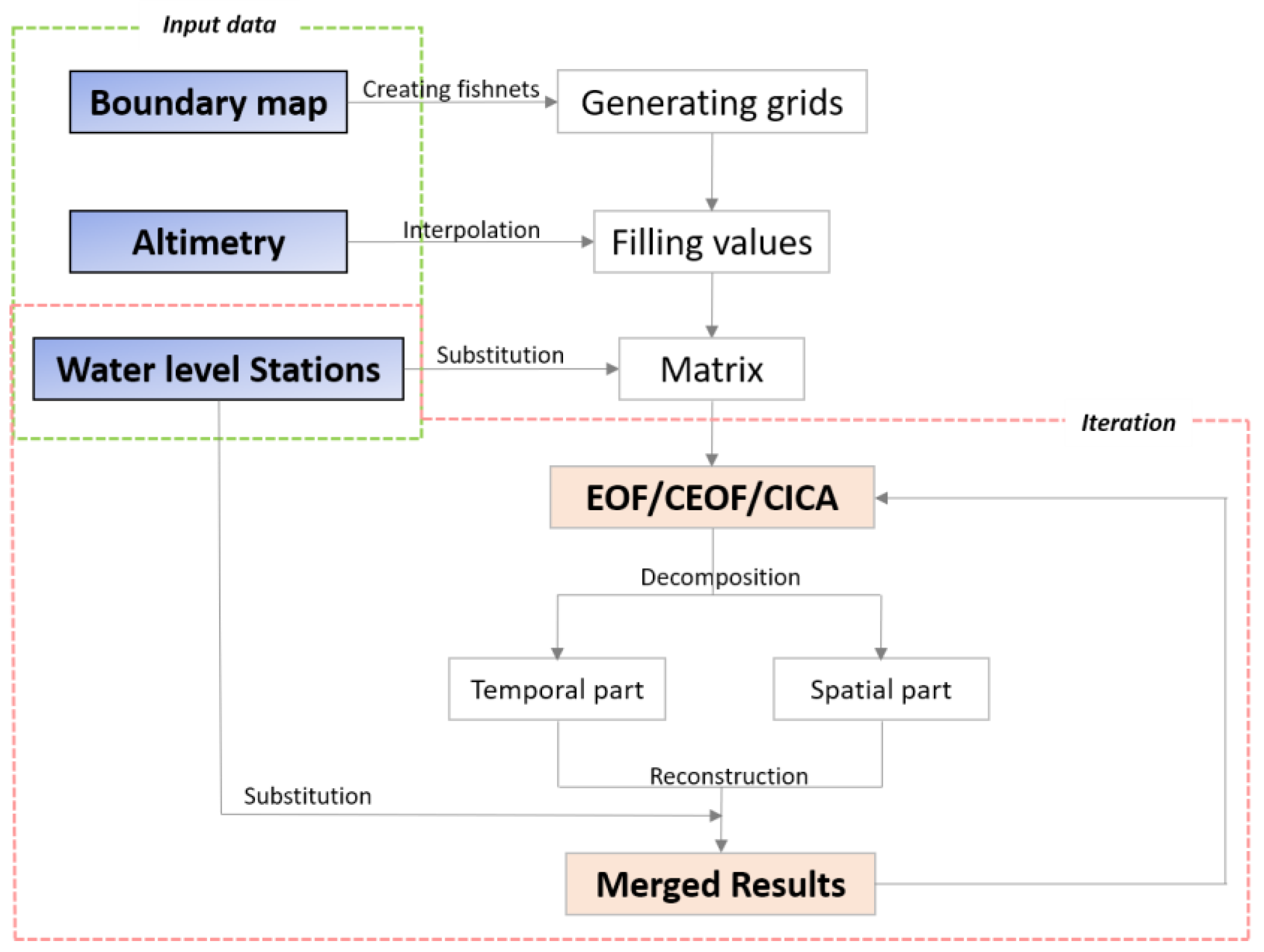
The target of our reconstruction procedures (Figure 3) was to generate regular water-level maps at ~10 km scale covering each lake from April 1984 to September 2018. The data acquisition procedure was as follows: (1) 0.1° × 0.1° grids were generated by ArcGIS software, and the grid points filled with available altimetry data geographically located near to the latitude and longitude of the specified grid, substituted by zero if data was missing; (2) a data matrix X was formulated that containing m (number of grid points) sampled time series with a length of n (number of epochs); (3) the zero entries in each row of the data matrix X were replaced by the median of the non-zero entries of the water level station data; (4) CICA/CEOF/EOF was applied to decompose the data matrix X into orthogonal or independent components; (5) the surface height of each lake was reconstructed by using reserved components from Step 4; (6) the former zero entries of Step 3 were replaced by the median obtained from Step 5, and a new X field generated; (7) Steps 5 and 6 were repeated until no considerable changes were detected in the modes of Step 4 or equivalent data matrix (X) of Step 6. Description of EOF, CEOF, and CICA is provided in Appendix A. Lake Erie was taken as the reconstruction example and the results are shown in the supplementary file. In this study, over 90% of total variance was observed in the first five, nine, and twelve modes decomposed by EOF, CEOF, and CICA, respectively (see Figures S1–S4). The iteration numbers were defined by the maximum correlation coefficients and minimum RMSE values (see Text S2 and Figure S5 in Supplementary).

3. Results

3.1. Effects of GIA on the Great Lakes

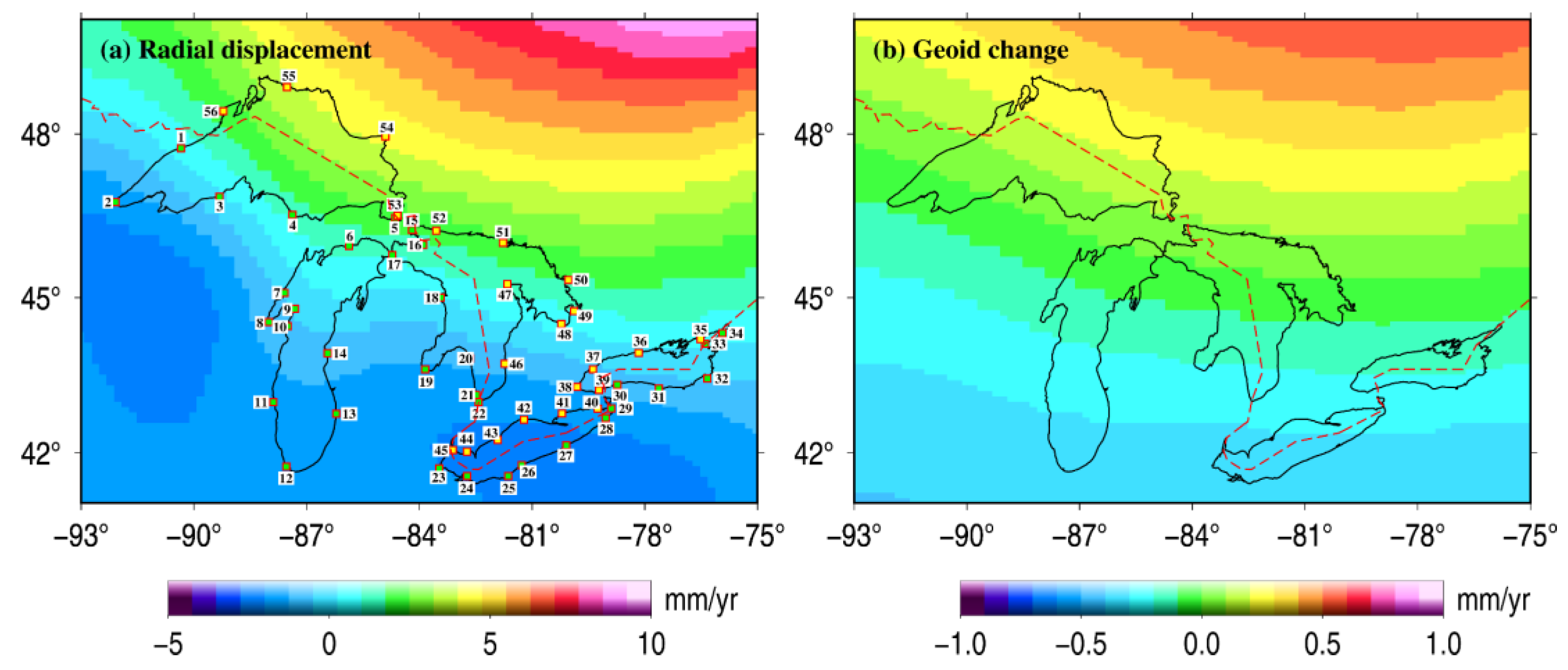
Figure 4a shows the radial displacement rate in the Great Lakes Basin according to the ICE-6G GIA model. Most of the stations located in the USA and southeastern Canada presented a negative ratio, while the radial displacement of southwestern Canadian stations gradually increased. Lake Superior, as the largest lake of the Great Lakes, was rising by 2.02 ± 2.85 mm/year (see in Table 1). However, the western region of the Lake Superior, accounting for roughly one third of its area, was subsiding; e.g., measurements at the #2 station, Duluth, were decreasing by about 1.50 mm/year. In contrast, all of Lake Erie, as the southernmost and smallest by volume of the Great Lakes, was falling by 2.07 ± 0.31 mm/year. For the other three lakes, overall displacement was not clear, but the southern parts of each presented positive values which were not negligible; e.g., measurements from the #12 station, the #22 station, and the #38 station were all decreasing at roughly 1–2 mm/year. Noticeably, at #54 station located in Canada, the rise was up to 140 mm from April 1985 to September 2018; the #24 station in USA reported a decrease of about 100 mm over the 33 years. In Figure 3b, the spatial distribution of geoid changes shows that the northeast of the Great Lakes was increasing while the southwestern part was decreasing. Although the magnitude of geoid change was smaller than radial displacement (see Table 1), we subtracted it to ensure consistency during the process of altimetry and in situ water level data calculation.

3.2. The Reconstructed Lake Surface Height

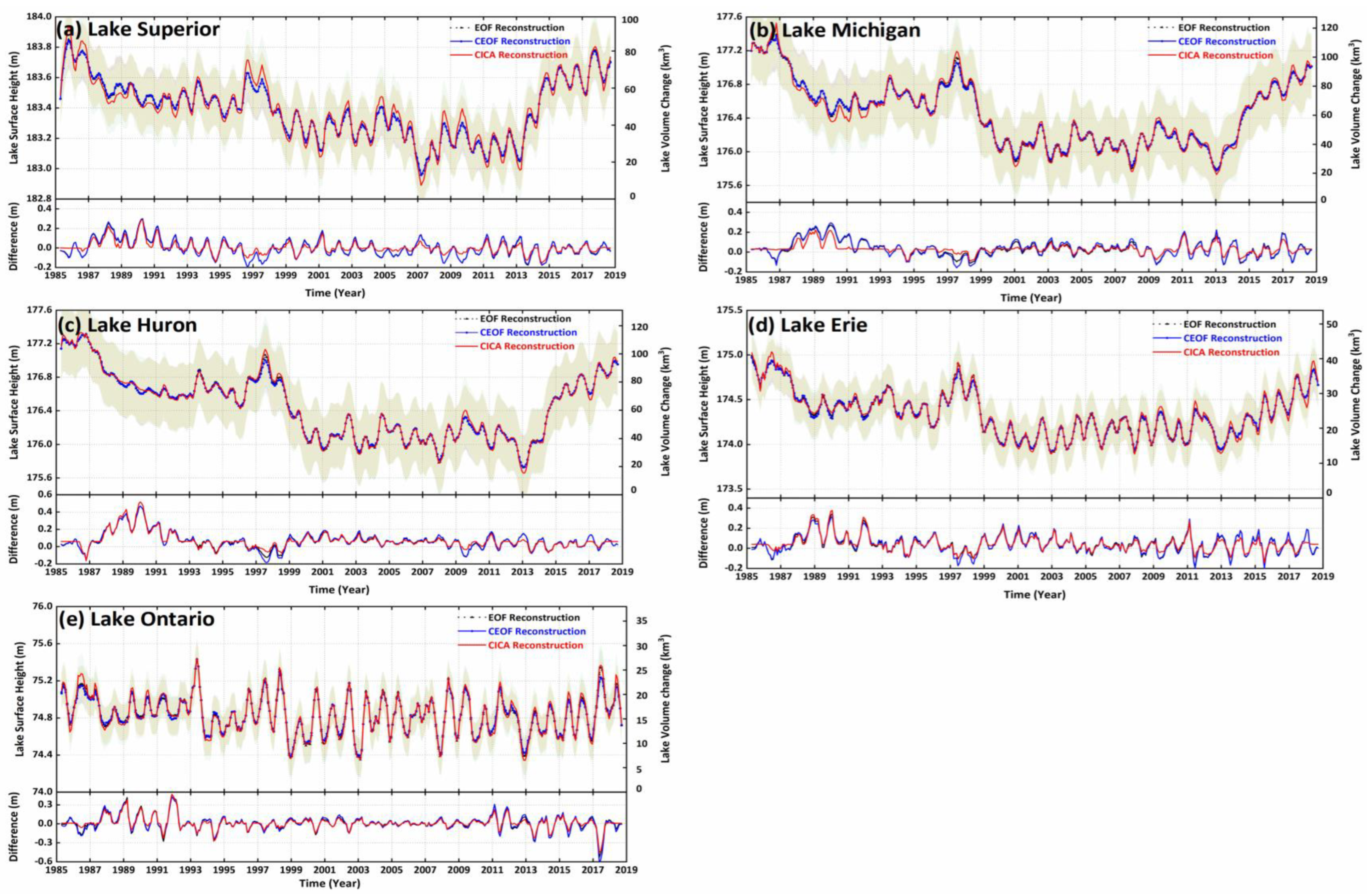
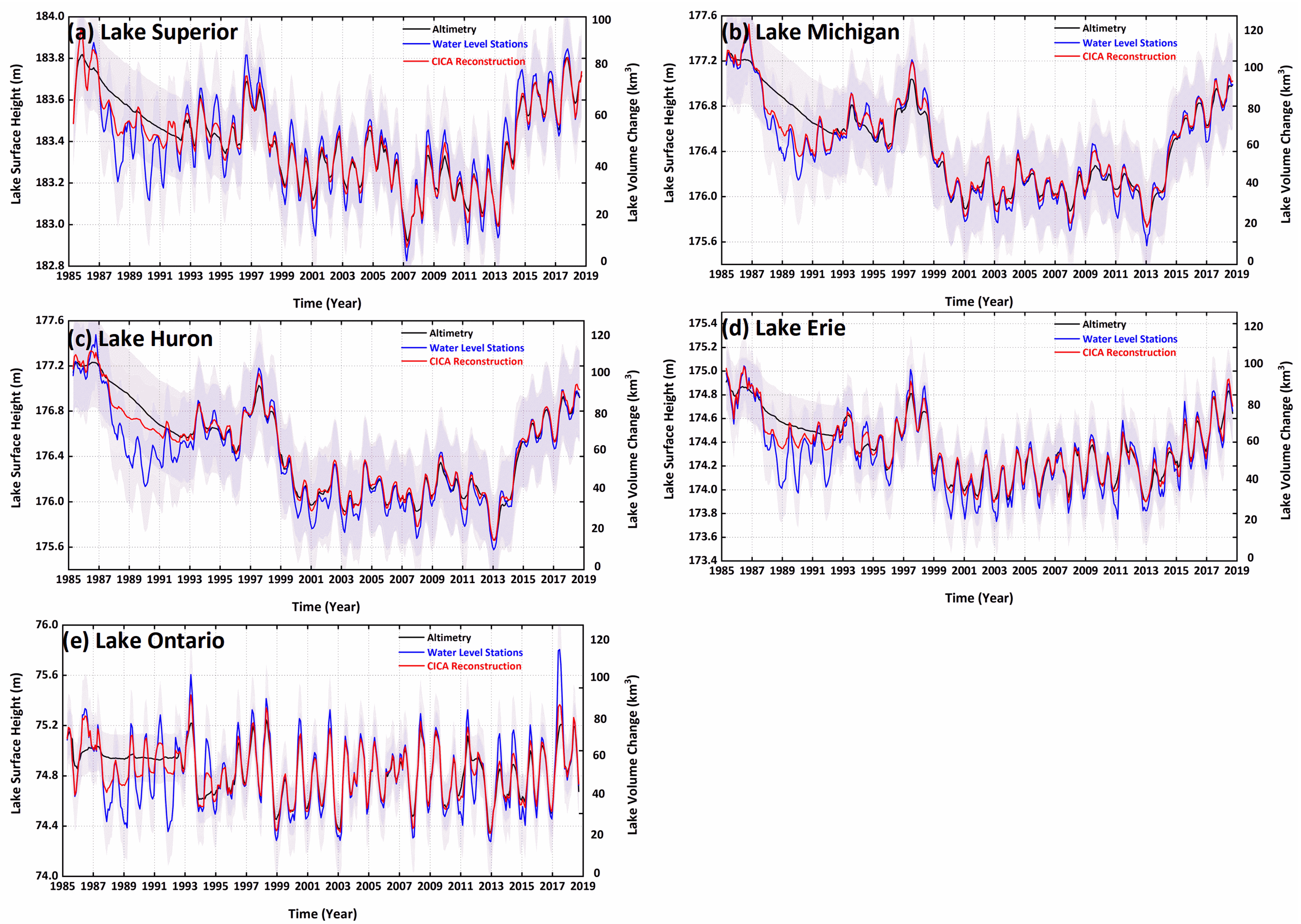
After removing the GIA effects, we re-estimated the entire lake level over the Great Lakes from April 1985 to September 2018. Figure 5a–e shows the Great Lakes’ time series for surface height and volume by EOF, CEOF, and CICA reconstruction, respectively. The subgraphs indicate the differences between the reconstructed results and the measurements from the water level stations. Figure 6a–e presents the results from the original altimetry estimations, water level stations, and CICA reconstruction, respectively. In general, all of them capture extreme fluctuations of water level in some time nodes; e.g., conspicuous positive peak values in El Niño years (1986/1987, 1997/1998) and negative peak values in La Niña years (1998/1999, 2007/2008, 2011/2012), which mainly appeared in Lakes Superior and Michigan, as well as 1997/1998 flooding in Lake Erie and 2017 flooding in Lake Ontario. The reconstructed results were more comparable with the water level station data, especially for the period 1986~1993 when there were less available good quality altimetry satellite data for the Great Lakes.
To compare the performance of different reconstructed methods, correlation coefficient and root mean square error (RMSE) were introduced. Table 2 shows the correlation coefficients and RMSE, with comparison of the reconstructed results, the original altimetry, and the in situ water level. These three reconstructed results had a higher correlation and lower RMSE with water level station data, presenting better performance results than the altimetry data.
For standard EOF reconstruction and CEOF reconstruction, it was difficult to distinguish which were the better results. EOF reconstruction performed slightly better than CEOF for Lake Superior, with higher correlation coefficients and RMSE, but STD for EOF was lower than for CEOF reconstruction. CEOF reconstruction performed slightly better than EOF for Lake Erie, but in Lake Michigan the correlation coefficient of EOF reconstruction was better than CEOF reconstruction, while the RMSE of CEOF reconstruction was better than EOF. Meanwhile, CICA reconstruction certainly performed better than the first two methods for each lake. The correlation coefficients of CICA reconstruction were all more than 0.95, and were even up to 0.99 for Lake Michigan. The RMSE of CICA reconstruction was up to 4.89 cm in Lake Superior and 6.07 cm in Lake Michigan, far less than the other two methods.
To verify the CICA technique as a higher order statistical decomposition method that can extract more independent and non-stationary components from the same explained covariances, performing better than the other two methods, Lake Erie is taken here as an instance for analysis (also see Figures S2–S5). For the modes decomposed by EOF and CEOF, only the first PC (principal components) presented lake surface changes when compared with the results of water level stations. In terms of the CICA’s modes, the sixth CIPC (complexed independent component) possibly suggests the existence of a multidecadal period which needs to be verified further; the eighth CIPC suggests a trend albeit contaminated with interannual variation; the ninth CIPC probably presents the lake level change recorded by altimetry, especially the obvious low-quality results in the period 1981~1992. Therefore, with more independent components including more inherent information about lake surface height, CICA’s results can be reconstructed and restored better than the commonly used EOF or CEOF.

4. Discussion

4.1. Corrections of Vertical Motion Resulting from GIA

For the impacts of GIA on the volumes of the Great Lakes, the maximum increase in volume was up to 0.65 m3/s in Lake Erie, while the maximum decrease in volume was 2.11 m3/s in Lake Michigan–Huron [49]. The apparent effect of GIA accounted for about 4 to 5 cm of the approximately 23 cm decline in difference between Lake Michigan–Huron and Lake Erie between 1963 and 2006 [50]. However, there were some differences among the different GIA models. In Table 3, we present the estimates of radial displacement averaged in each lake using the ICE-6G model, ICE-5G model, ICE-4G model, ICE-3G GIA model, and water level stations’ relative vertical motion. There were good agreements between different models for Lake Superior and Lake Michigan–Huron; but discrepancies for Lake Erie and especially Lake Ontario. This may be due to the limited availability of GPS sites in the region constraining the GIA models. With gradual improvement of the Continually Operating Reference Stations (CORS) network across the Great Lakes, we expect more accurate observations of vertical motion from these stations.

4.2. Impacts from ENSO on the Great Lakes

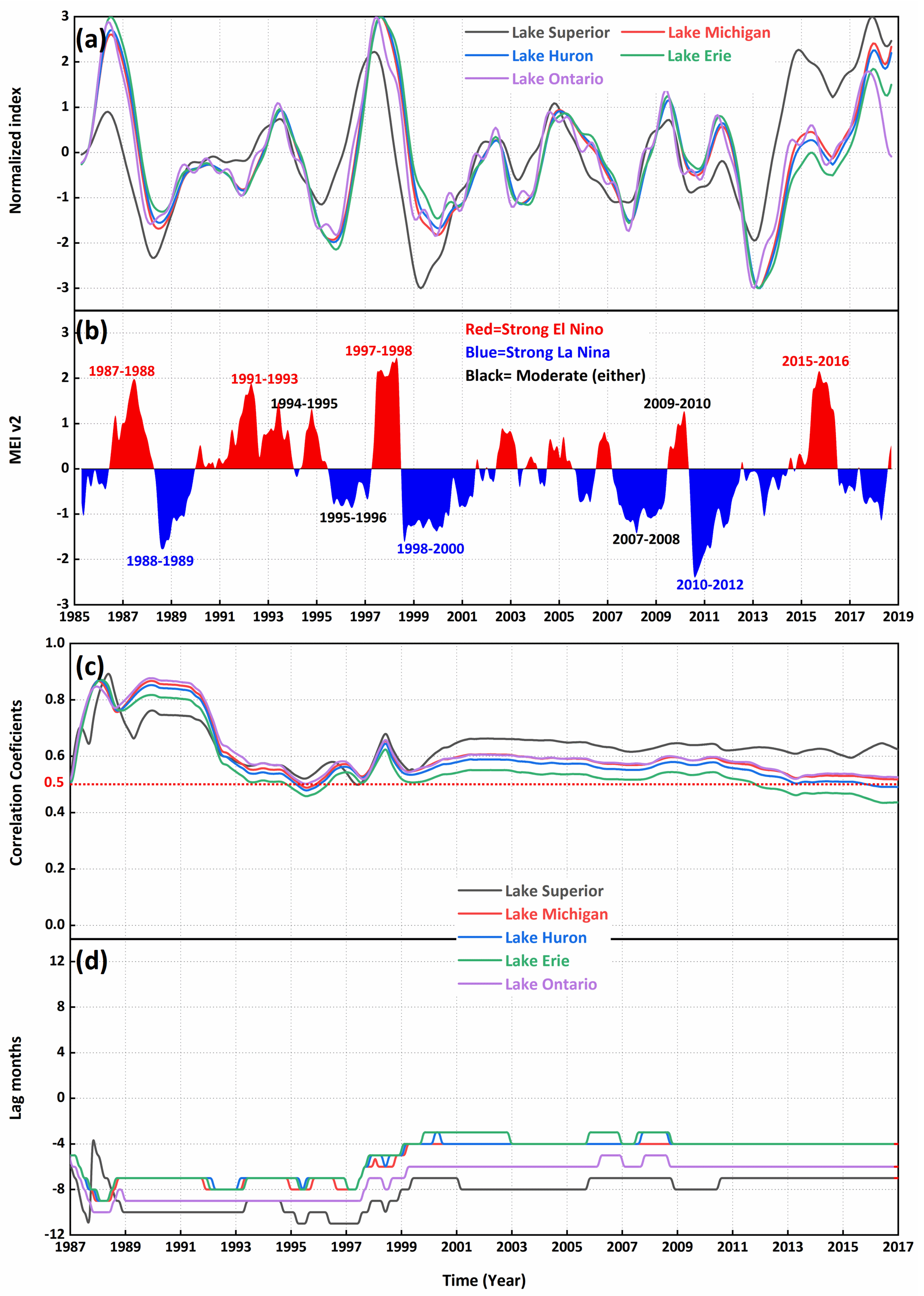
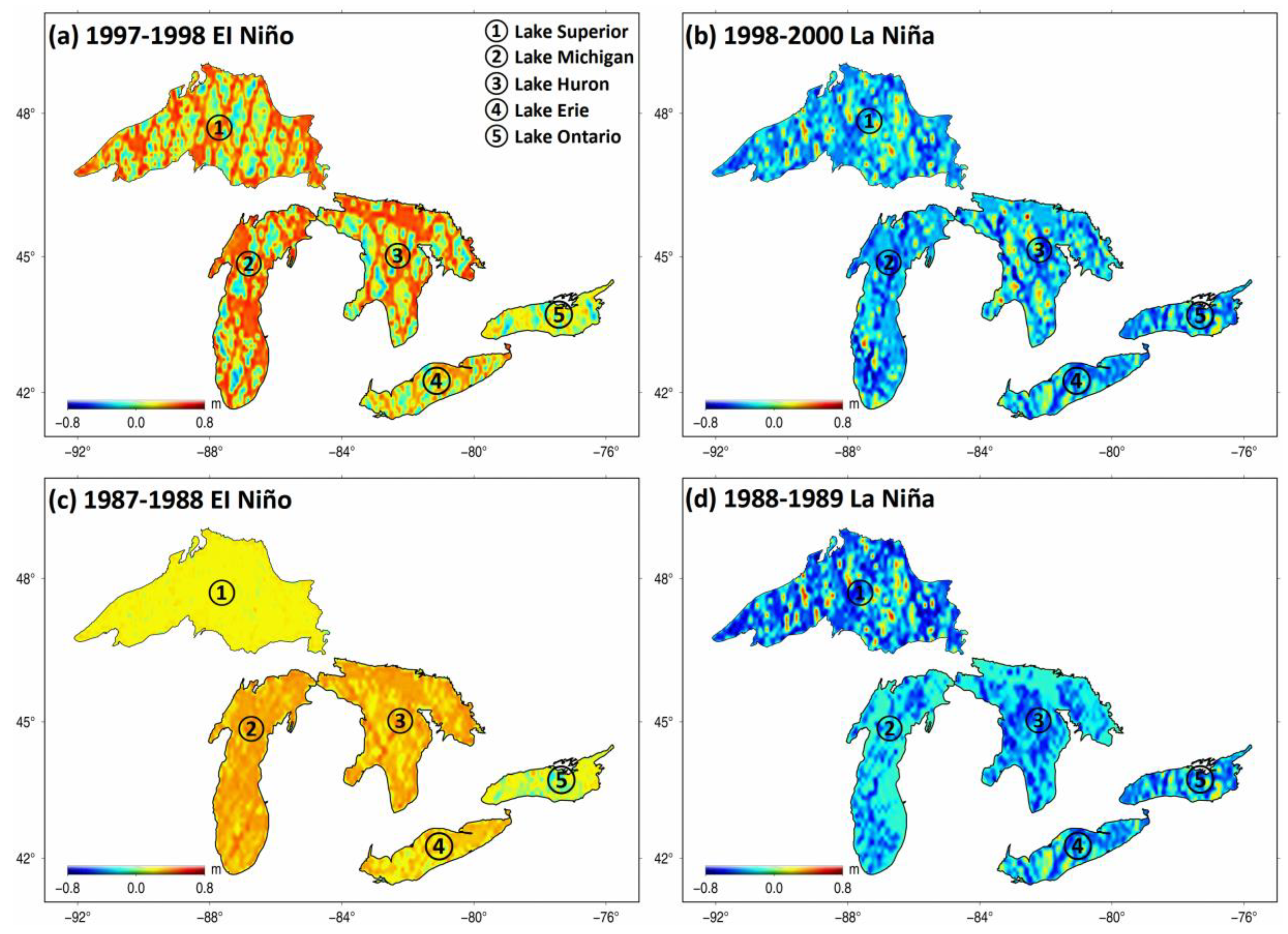
Previous studies have found that ENSO can affect ice cover [51], snowfall [52], air concentration [53], and precipitation [54] over the Great Lakes. In this study, we found that some peaks or ebbs of lake level happened during ENSO years, which were rarely mentioned in previous studies. The multi-channel singular spectrum analysis (M-SSA) method, which has been proved capable of decomposing the interannual components of multiple time-series [55], was applied to extract the interannual lake level from CICA reconstructions. A description of MSSA is given in Appendix B. The first five modes which occupied >90% explained variance (see Figure S6) was retained here. The second mode (see Figure S7) applies to the interannual variations of lake surface height. In Figure 7a,b, we show the time series of normalized interannual lake levels and MEI. The interannual anomalies occurred as high peaks before the warm phase of ENSO (i.e., El Niño), especially in 1987–1988, 1997–1998, and 2015–2016, while low ebb conditions were experienced before La Niña events, especially in 1988–1989, 1998–2000, and 2007–2008. Figure 8 presents the spatial fluctuations of lake levels during the periods of 1997–1998 EI Niño, 1998–2000 La Niña, 1987–1988 EI Niño, and 1988–1989 La Niña. After abstracting the targeted signal during the period of ENSO, we found that the lake levels were ~25 cm higher than normal during EI Niño events, and ~30 cm lower than normal during La Niña. In addition, different spatial anomalies of interannual lake level were possibly caused by various types of ENSO events. Different ENSO-type influences will be further studied from the perspective of water balance, including terrestrial water storage, precipitation, and evaporation over the Great Lakes.
Figure 7c,d shows the maximum correlation coefficients and lag months. There were positive correlations, generally higher than 0.5 with 95% CI, between the normalized interannual lake level and MEI over the Great Lakes. Note that first and last two years’ data were not considered in the calculation, to avoid the possible boundary effect in correlation analysis. During 1999–2011, these correlation coefficients and lag months remained stable, which were from 0.5–0.6 and 4–6 months, respectively, for four lakes (Michigan, Ontario, Huron, and Erie), and 0.6–0.7 and 7–8 months for Lake Superior. The correlations begin to decline after 2011, lower than 0.5 for Lake Erie. The decrease of correlation coefficients may indicate that the Lake Erie has also been affected by other climatic or anthropogenic influences in recent years.

5. Conclusions

In this study, the spatio-temporal changes of lake surface heights in the Great Lakes from April 1985 to September 2018 were reconstructed. Before reconstruction, GIA corrections were taken into consideration to ensure data consistency. In terms of GIA corrections, the radial displacement resulting from GIA was found to contribute 2.02 ± 2.85 mm/year in Lake Superior, and −2.07 ± 0.31 mm/year in Lake Erie. After removing the effect of GIA, we used three methods (EOF reconstruction, CEOF reconstruction, and CICA reconstruction) to reconstruct the lake surface levels. CICA reconstruction was proposed as a new iterative reconstruction method, and its improved performance over EOF reconstruction and CEOF reconstruction was demonstrated: the correlation coefficient with water level stations reached 0.97, 0.99, 0.97, 0.97, and 0.95, respectively, and the RMSE during the study period was 6.07 cm, 4.89 cm, 9.27 cm, 7.71 cm, and 9.88 cm, respectively. The interannual variations of water level were further investigated in terms of their connections with ENSO, revealing that the Great Lakes are significantly affected by ENSO. The lake levels were higher than normal in the years of EI Niño, and lower in the years of La Niña. The maximal correlation coefficients between lake levels and MEI were 0.5–0.6 with leading of 4–6 months over four lakes (Lake Michigan, Lake Ontario, Lake Huron, and Lake Erie) and 0.6–0.7 with leading of 7–8 months over Lake Superior. With development in the near future of altimetry satellites with better spatio-temporal resolution and coverage, we hope to use the reconstructed method to monitor transient changes of water level, and provide support for decision-making for water resources management and regulation, floodwater observations, and discharge in the Great Lakes.

Supplementary Materials

The following supporting information can be downloaded at: https://www.mdpi.com/article/10.3390/rs14205194/s1, Figure S1: cumulative percentage of total variance accounted by the first several modes by EOF, CEOF, and CICA; Figures S2–S4: the retained spatial patterns and temporal components from EOF, CEOF, and CICA, respectively; Figure S5: relationships between iteration numbers, the correlation coefficients, and RMSE values; Figure S6: cumulative percentage of the total variance by MSSA; Figure S7: modes kept by MSSA. References [56,57] are cited in the Supplementary Materials.

Author Contributions

E.F., C.K.S. and W.F. designed the experiment; W.C. conducted the experiments; W.C. wrote the manuscript; W.F., C.K.S., E.F. and J.G. revised the manuscript; Y.J., C.W., W.L. and Q.L. collected and analyzed parts of the data; M.Z., W.F. and L.L. provided financial support and rationalized the logic of the manuscript. All authors have read and agreed to the published version of the manuscript.

Funding

National Natural Science Foundation of China (41874095, 41704013, 42061134010). Strategic Priority Research Program of the Chinese Academy of Sciences (XDA20100300, XDA15017700). Max-Planck-Society and the Chinese Academy of Sciences within the LEGACY (“Low-Frequency Gravitational Wave Astronomy in Space”) collaboration (M.IF.A. QOP18098); Natural Science Fund for Distinguished Young Scholars of Hubei Province, China (2019CFA09); Danmarks Frie Forskningsfond (10.46540/2035-00247B). Cooperative Institute for Great Lakes Research (SUBK00011366).

Acknowledgments

We thank Philip Chu, NOAA’s Great Lakes Environmental Research Laboratory, USA for his technical and financial support. Wei Chen acknowledges the China Scholarship Council’s scholarship support. Wei Feng acknowledges support from the International Space Science Institute (ISSI, Bern, CH) and ISSI-BJ (Beijing, CN) through the team on “Time-Variable Gravity Field Modeling and Simulation from Present and Future Gravity Satellite Missions”. Ehsan Forootan acknowledges Danmark’s Frie Forskningsfond [10.46540/2035-00247B] through the DANSk-LSM project.

Conflicts of Interest

The authors declare no conflict of interest.

Appendix A. Description of EOF/CEOF/CICA

Empirical orthogonal function (EOF), as a common statistical signal decomposition technique, is widely applied to extract orthogonal modes from observations that represent the dominant part of the variance [58,59]. Here, EOF is described again because it was the basis for the subsequent two methods. First, the data matrix X was prepared (see Section 2.6) containing xi = [x1i, x2i, …, xni]T; i = 1, …, p in its columns. Then, after removing column-wise temporal means of X, the auto-covariance matrix (containing variances and covariances between time series of any pairs of grid points) was computed from the Equation (A1):
C = 1 n X T X
The aim of EOF is to find directions such as e = ( e 1 , e 2 , …)T in the data. In that case, the vector e is an eigenvector of the matrix C, and all possible directions of e are stored in the matrix E . Finally, we reconstructed the data matrix by retaining the dominant orthogonal modes, i.e., X j = P j E j T , where j ≤ min (n, p) is the number of retained modes, P j stores the principal components in its columns (PTP = ∧2, ∧ represents the square roots of the eigenvalues of C), E j contains orthogonal base functions, and X j is therefore an approximation of X.
Complex empirical orthogonal function (CEOF) is an alternative to EOF, and can extract non-stationary patterns. Here, the Hilbert transformation was introduced to develop CEOF, by introducing a complex field. The data matrix X (shown by X t ) can be assumed as a scalar filed with discrete Fourier representation of Equation (A2):
X t = w k ( a ( w k ) cos ( w k t ) + b ( w k ) sin ( w k t ) ) ,   t = 1 , , n
where a ( w k ) and b ( w k ) are the vector of Fourier coefficients at frequency w k (with accepting values between −π and π selected according to the sampling rate). Notably, values of w k need to satisfy the Nyquist frequency rule, and its equivalent wavelength should not exceed the length of time series. Then, the Hilbert transform (H) of X t is given by Equation (A3):
H ( X t ) = w k ( b ( w k ) cos ( w k t ) a ( w k ) sin ( w k t ) ) ,   t = 1 , , n
A new complexified data matrix can be defined as: Y t = X t + i∙H( X t ), where i = 1 . Therefore, the real part of the complexified matrix is the original data matrix and its imaginary part is its Hilbert transform. Here, the auto-covariance matrix can be computed from Equation (A4):
C = 1 n ( Y t T Y t ) = ( X T X + H ( X ) T H ( X ) + i · ( X T H ( X ) H ( X ) T X ) )
The new covariance matrix is decomposing into orthogonal modes of P and E that now contain complex entries. Finally, matrix X j can be estimated in a similar manner to the EOF method, i.e., X j = Re ( P j E j T ) , where Re(.) is an operator that extracts the real part of the complex numbers.
Second-order statistical signal-decomposition methods (EOF and CEOF) have been previously described. To incorporate more information from the probability density function (PDF) underlying the data and improve the identification of non-stationary patterns, complex independent component analysis (CICA) is proposed as a higher statistical decomposition method. Similar to CEOF, the data matrix X is transformed by Equations (A2) and (A3), and complex orthogonal components are obtained by Equation (A4). Then, the reconstructed formulation of CICA can be written as:
X j = Re ( P j R j   R j T E j ) = Re ( P j Y E j Y T )
a new pair of base functions P j Y and E j Y are defined ( P j Y = P j R j , E j Y = R j T E j R j R j T = I , I is an identical matrix). Here, a proper rotation matrix R j needs to be defined to guarantee the independence of P j Y   and   E j Y T . Thus, fourth-order cumulants are necessarily introduced based on the complex value as
C ( x i , x j * , x k , x l * ) = E ( x i x j * · x k x l * ) E ( x i x j * ) E ( x k x l * ) E ( x i x k ) E ( x j * x l * ) E ( x i x l * ) E ( x k x j * )
where E(.) is the expectation operator, * represents the complex conjugate, and x represents a column of P j Y or E j Y . Accordingly, the fourth-order cumulant tensors originate from Equation (A7):
Q ( M ) = E ( ( x * Mx ) x * x ) C · trace ( M · C ) C · ( M + M T ) · C
where C is the auto-covariance matrix of variables x, M is an arbitrary matrix defined to store the cumulants. Finally, the required rotation R j for diagonalizing was computed by the joint diagonalization (JD) approach described in [60,61].

Appendix B. Description of M-SSA

Here, we briefly describe the multi-channel singular spectrum analysis (M-SSA) method; the detailed descriptions can be found Ghil et al. (2002) [62] and Groth et al. (2011) [55]. First, let x i   ( 1 i L ) be a time-series of length L, the column of x i is N. Then, we can construct the matrix:
D ˜ j = [ X i ( 1 ) X i ( 2 ) X i ( M ) X i ( 2 ) X i ( 3 ) X i ( M + 1 ) X i ( N ) X i ( N + 1 ) X i ( N ) ]
where N = N M + 1 , after considering a window M ( 1 < M < N ). For M-SSA, the covariance matrix can be also obtained by Equation (A9):
T i , j = 1 N D ˜ i T D ˜ j
Likewise, we can project X i ( n ) onto the spatio-temporal empirical orthogonal functions (ST-EOFs) to obtain the corresponding spatio-temporal principal components (ST-PCs), based on Equation (A10),
A K ( n ) = j = 1 M i = 1 L X i ( n + j 1 ) E i K ( j ) ,   1 n N
where E K is the Kth eigenvector of T . Each independent signal R can also be obtained by Equation (A11):
R i K ( n ) = { 1 n j = 1 n A K ( n j + 1 ) E i K ( j ) , 1 n M 1 1 M j = 1 M A K ( n j + 1 ) E i K ( j ) , M n N 1 N n + 1 j = n N + M M A K ( n j + 1 ) E i K ( j ) ,     N + 1 n N

References

  1. Waples, J.T.; Eadie, B.; Klump, J.V.; Squires, M.; Cotner, J.; McKinley, G. The Laurentian Great Lakes. In Continental Margins: A Synthesis and Planning Workshop, North American Continental Margins Working Group for the US Carbon Cycle Scientific Steering Group and Interagency Working Group; US Carbon Cycle Program: Washington, DC, USA, 2008; pp. 73–81. Available online: http://www.glerl.noaa.gov/pubs/fulltext/2008/20080024.pdf (accessed on 15 December 2020).
  2. Gershunov, A.; Barnett, T.P. Interdecadal modulation of ENSO teleconnections. Bull. Am. Meteorol. Soc. 1998, 79, 2715–2726. [Google Scholar] [CrossRef]
  3. De Loë, R.C.; Kreutzwiser, R.D. Climate Variability, Climate Change and Water Resource Management in the Great Lakes. Clim. Chang. 2000, 45, 163–179. [Google Scholar] [CrossRef]
  4. Gronewold, A.D.; Stow, C.A. Water Loss from the Great Lakes. Science 2014, 343, 1084–1085. [Google Scholar] [CrossRef] [PubMed]
  5. Yang, G.; Bowling, L.C. Detection of changes in hydrologic system memory associated with urbanization in the Great Lakes region. Water Resour. Res. 2014, 50, 3750–3763. [Google Scholar] [CrossRef]
  6. Quinn, F.H. Secular changes in Great Lakes water level seasonal cycles. J. Great Lakes Res. 2002, 28, 451–465. [Google Scholar] [CrossRef]
  7. Burton, T.M. The effects of water level fluctuations on Great Lakes coastal marshes. In Coastal Wetlands; Lewis Publishers: Chelsea, MI, USA, 2018; pp. 3–13. [Google Scholar]
  8. Kayastha, M.B.; Ye, X.; Huang, C.; Xue, P. Future rise of the Great Lakes water levels under climate change. J. Hydrol. 2022, 612, 128205. [Google Scholar] [CrossRef]
  9. Gronewold, A.D.; Rood, R.B. Recent water level changes across Earth’s largest lake system and implications for future variability. J. Great Lakes Res. 2019, 45, 1–3. [Google Scholar] [CrossRef]
  10. Hwang, C.; Peng, M.-F.; Ning, J.; Luo, J.; Sui, C.-H. Lake level variations in China from TOPEX/Poseidon altimetry: Data quality assessment and links to precipitation and ENSO. Geophys. J. Int. 2005, 161, 1–11. [Google Scholar] [CrossRef] [Green Version]
  11. Wang, H.; Chu, Y.; Huang, Z.; Chao, N. Robust, Long-term Lake Level Change from Multiple Satellite Altimeters in Tibet: Observing the Rapid Rise of Ngangzi Co over a New Wetland. Remote Sens. 2019, 11, 558. [Google Scholar] [CrossRef] [Green Version]
  12. Sun, M.; Guo, J.; Yuan, J.; Liu, X.; Wang, H.; Li, C. Detecting Lake Level Change From 1992 to 2019 of Zhari Namco in Tibet Using Altimetry Data of TOPEX/Poseidon and Jason-1/2/3 Missions. Front. Earth Sci. 2021, 9, 640553. [Google Scholar] [CrossRef]
  13. Herdendorf, C.E. Great lakes estuaries. Estuaries 1990, 13, 493–503. [Google Scholar] [CrossRef]
  14. Ault, T.W.; Czajkowski, K.P.; Benko, T.; Coss, J.; Struble, J.; Spongberg, A.; Templin, M.; Gross, C. Validation of the MODIS snow product and cloud mask using student and NWS cooperative station observations in the Lower Great Lakes Region. Remote Sens. Environ. 2006, 105, 341–353. [Google Scholar] [CrossRef]
  15. Morris, C.S.; Gill, S.K. Variation of Great Lakes water levels derived from Geosat altimetry. Water Resour. Res. 1994, 30, 1009–1017. [Google Scholar] [CrossRef]
  16. Jekeli, C.; Dumrongchai, P. On monitoring a vertical datum with satellite altimetry and water-level gauge data on large lakes. J. Geodesy 2003, 77, 447–453. [Google Scholar] [CrossRef]
  17. Kuo, C.-Y.; Shum, C.; Braun, A.; Cheng, K.-C.; Yi, Y. Vertical Motion Determined Using Satellite Altimetry and Tide Gauges. Terr. Atmospheric Ocean. Sci. 2008, 19, 21–35. [Google Scholar] [CrossRef] [Green Version]
  18. Cheng, K.-C.; Kuo, C.-Y.; Tseng, H.-Z.; Yi, Y.; Shum, C. Lake Surface Height Calibration of Jason-1 and Jason-2 Over the Great Lakes. Mar. Geodesy 2010, 33, 186–203. [Google Scholar] [CrossRef]
  19. Jia, Y.; Shum, C.K.; Chu, P. Monitoring water level variations over the Great Lakes using contemporary satellite geodetic observations. In AGU Fall Meeting Abstracts; AGU Publisher: Washington, DC, USA, 2018; p. H31K-2074. [Google Scholar]
  20. Alsdorf, D.E.; Rodríguez, E.; Lettenmaier, D.P. Measuring surface water from space. Rev. Geophys. 2007, 45, RG2002. [Google Scholar] [CrossRef]
  21. Lee, H.; Beighley, R.E.; Alsdorf, D.; Jung, H.C.; Shum, C.; Duan, J.; Guo, J.; Yamazaki, D.; Andreadis, K. Characterization of terrestrial water dynamics in the Congo Basin using GRACE and satellite radar altimetry. Remote Sens. Environ. 2011, 115, 3530–3538. [Google Scholar] [CrossRef] [Green Version]
  22. Smith, T.M.; Reynolds, R.W.; Livezey, R.E.; Stokes, D.C. Reconstruction of historical sea surface temperatures using empirical orthogonal functions. J. Clim. 1996, 9, 1403–1420. [Google Scholar] [CrossRef]
  23. Wenzel, M.; Schröter, J. Reconstruction of regional mean sea level anomalies from tide gauges using neural networks. J. Geophys. Res. Earth Surf. 2010, 115, C08013. [Google Scholar] [CrossRef]
  24. Kaplan, A.; Kushnir, Y.; Cane, M.A. Reduced Space Optimal Interpolation of Historical Marine Sea Level Pressure: 1854–1992. J. Clim. 2000, 13, 2987–3002. [Google Scholar] [CrossRef]
  25. Chambers, D.P.; Mehlhaff, C.A.; Urban, T.J.; Fujii, D.; Nerem, R.S. Low-frequency variations in global mean sea level: 1950–2000. J. Geophys. Res. Ocean. 2002, 107, 1-1–1-10. [Google Scholar] [CrossRef]
  26. Church, J.A.; White, N.J.; Coleman, R.; Lambeck, K.; Mitrovica, J.X. Estimates of the regional distribution of sea level rise over the 1950–2000 period. J. Clim. 2004, 17, 2609–2625. [Google Scholar] [CrossRef]
  27. Hamlington, B.D.; Cheon, S.H.; Thompson, P.R.; Merrifield, M.A.; Nerem, R.S.; Leben, R.R.; Kim, K.Y. An ongoing shift in Pacific Ocean Sea level. J. Geophys. Res. Ocean. 2016, 121, 5084–5097. [Google Scholar] [CrossRef] [Green Version]
  28. Forootan, E. Statistical Signal Decomposition Techniques for Analyzing Time-Variable Satellite Gravimetry Data. Ph.D. Thesis, Universitäts-und Landesbibliothek Bonn, Bonn, Germany, 2014. [Google Scholar]
  29. Von Storch, H.; Navarra, A. (Eds.) Analysis of Climate Variability: Applications of Statistical Techniques; Springer Science & Business Media: Berlin/Heidelberg, Germany, 1999. [Google Scholar]
  30. Forootan, E.; Kusche, J.; Talpe, M.; Shum, C.K.; Schmidt, M. Developing a Complex Independent Component Analysis (CICA) Technique to Extract Non-stationary Patterns from Geophysical Time Series. Surv. Geophys. 2017, 39, 435–465. [Google Scholar] [CrossRef] [Green Version]
  31. Horel, J.D. Complex Principal Component Analysis: Theory and Examples. J. Clim. Appl. Meteorol. 1984, 23, 1660–1673. [Google Scholar] [CrossRef]
  32. Von Storch, H. Misuses of statistical analysis in climate research. In Analysis of Climate Variability; Springer: Berlin/Heidelberg, Germany, 1999; pp. 11–26. [Google Scholar]
  33. Merrifield, M.A.; Guza, R.T. Detecting Propagating Signals with Complex Empirical Orthogonal Functions: A Cautionary Note. J. Phys. Oceanogr. 1990, 20, 1628–1633. [Google Scholar] [CrossRef]
  34. Hannachi, A.; Jolliffe, I.; Stephenson, D. Empirical orthogonal functions and related techniques in atmospheric science: A review. Int. J. Climatol. A J. R. Meteorol. Soc. 2007, 27, 1119–1152. [Google Scholar] [CrossRef]
  35. Aires, F.; Rossow, W.; Scott, N.; Chedin, A. Remote sensing from the infrared atmospheric sounding interferometer instrument 2. Simultaneous retrieval of temperature, water vapor, and ozone atmospheric profiles. J. Geophys. Res. Earth Surf. 2002, 107, ACH 7-1–ACH 7-12. [Google Scholar] [CrossRef]
  36. Forootan, E.; Kusche, J. Separation of global time-variable gravity signals into maximally independent components. J. Geodesy 2011, 86, 477–497. [Google Scholar] [CrossRef]
  37. Westra, S.; Brown, C.; Lall, U.; Sharma, A. Modeling multivariable hydrological series: Principal component analysis or independent component analysis? Water Resour. Res. 2007, 43, W06429. [Google Scholar] [CrossRef] [Green Version]
  38. Hyvärinen, A.; Oja, E. Independent component analysis: Algorithms and applications. Neural Netw. 2000, 13, 411–430. [Google Scholar] [CrossRef] [Green Version]
  39. Forootan, E.; Awange, J.; Kusche, J.; Heck, B.; Eicker, A. Independent patterns of water mass anomalies over Australia from satellite data and models. Remote Sens. Environ. 2012, 124, 427–443. [Google Scholar] [CrossRef] [Green Version]
  40. Williamson, J. The Inland Seas of North America: And the Natural and Industrial Productions of Canada, with the Real Foundations for Its Future Prosperity; Duff, J., Ed.; H. Ramsay: Montreal, QC, Cananda, 1854. [Google Scholar]
  41. Dolan, D.M.; Chapra, S.C. Great Lakes total phosphorus revisited: 1. Loading analysis and update (1994–2008). J. Great Lakes Res. 2012, 38, 730–740. [Google Scholar] [CrossRef]
  42. Birkett, C. The contribution of TOPEX/POSEIDON to the global monitoring of climatically sensitive lakes. J. Geophys. Res. Earth Surf. 1995, 100, 25179–25204. [Google Scholar] [CrossRef]
  43. Gronewold, A.D.; Fortin, V.; Lofgren, B.; Clites, A.; Stow, C.A.; Quinn, F. Coasts, water levels, and climate change: A Great Lakes perspective. Clim. Chang. 2013, 120, 697–711. [Google Scholar] [CrossRef]
  44. Simons, M.; Hager, B.H. Localization of the gravity field and the signature of glacial rebound. Nature 1997, 390, 500. [Google Scholar] [CrossRef]
  45. Peltier, W.; Argus, D.; Drummond, R. Space geodesy constrains ice age terminal deglaciation: The global ICE-6G_C (VM5a) model. J. Geophys. Res. Solid Earth 2015, 120, 450–487. [Google Scholar] [CrossRef] [Green Version]
  46. Trenberth, K.; Jones, P.; Ambenje, P.; Bojariu, R.; Easterling, D.; Klein Tank, A.; Parker, D.; Rahimzadeh, F.; Renwick, J.; Rusticucci, M. Observations: Surface and atmospheric climate change. In Climate Change; Cambridge University Press: Cambridge, UK, 2007; pp. 235–336. [Google Scholar]
  47. Cayan, D.R.; Redmond, K.T.; Riddle, L.G. ENSO and Hydrologic Extremes in the Western United States. J. Clim. 1999, 12, 2881–2893. [Google Scholar] [CrossRef]
  48. Li, X.; Zhong, S.; Bian, X.; Heilman, W. Climate and climate variability of the wind power resources in the Great Lakes region of the United States. J. Geophys. Res. Earth Surf. 2010, 115, 1–15. [Google Scholar] [CrossRef]
  49. Gill, S.K. Gap Analysis of the Great Lakes Component of the National Water Level Observation Network; NOAA: Silver Spring, MD, USA, 2014. [Google Scholar]
  50. Bruxer, J.; Southam, C. Analysis of Great Lakes Volume Changes Resulting from Glacial Isostatic Adjustment. In Data Technical Work Group; International Upper Great Lakes Study: Burlington, VT, USA, 2008. [Google Scholar]
  51. Wang, J.; Bai, X.; Hu, H.; Clites, A.; Colton, M.; Lofgren, B. Temporal and Spatial Variability of Great Lakes Ice Cover, 1973–2010. J. Clim. 2012, 25, 1318–1329. [Google Scholar] [CrossRef]
  52. Kunkel, K.E.; Angel, J.R. Relationship of ENSO to snowfall and related cyclone activity in the contiguous United States. J. Geophys. Res. Earth Surf. 1999, 104, 19425–19434. [Google Scholar] [CrossRef]
  53. Ma, J.; Venkatesh, S.; Jantunen, L. Evidence of the impact of ENSO events on temporal trends of hexachlorobenzene air concentrations over the Great Lakes. Sci. Total Environ. 2003, 313, 177–184. [Google Scholar] [CrossRef]
  54. Smith, S.R.; Legler, D.M.; Remigio, M.J.; O’Brien, J.J. Comparison of 1997–98 U.S. Temperature and Precipitation Anomalies to Historical ENSO Warm Phases. J. Clim. 1999, 12, 3507–3515. [Google Scholar] [CrossRef]
  55. Groth, A.; Ghil, M. Multivariate singular spectrum analysis and the road to phase synchronization. Phys. Rev. E 2011, 84, 036206. [Google Scholar] [CrossRef] [PubMed] [Green Version]
  56. Alvera-Azcárate, A.; Barth, A.; Rixen, M.; Beckers, J.M. Reconstruction of incomplete oceanographic data sets using empirical orthogonal functions: Application to the Adriatic Sea surface temperature. Ocean. Model. 2005, 94, 325–346. [Google Scholar] [CrossRef] [Green Version]
  57. Erhardt, E.B.; Rachakonda, S.; Bedrick, E.J.; Allen, E.A.; Adali, T.; Calhoun, V.D. Comparison of multi-subject ICA methods for analysis of fMRI data. Hum. Brain Mapp. 2011, 3212, 2075–2095. [Google Scholar] [CrossRef] [Green Version]
  58. Pandžić, K.; Likso, T. Eastern Adriatic typical wind field patterns and large-scale atmospheric conditions. Int. J. Clim. 2005, 25, 81–98. [Google Scholar] [CrossRef]
  59. Yang, W.; Zhao, Y.; Wang, D.; Wu, H.; Lin, A.; He, L. Using Principal Components Analysis and IDW Interpolation to Determine Spatial and Temporal Changes of Surface Water Quality of Xin’anjiang River in Huangshan, China. Int. J. Environ. Res. Public Health 2020, 17, 2942. [Google Scholar] [CrossRef]
  60. Cardoso, J.F.; Souloumiac, A. Blind beamforming for non-Gaussian signals. Proc. IEEE 1993, 140, 362–370. [Google Scholar] [CrossRef]
  61. Cardoso, J.F.; Souloumiac, A. Jacobi angles for simultaneous diagonalization. SIAM J. Matrix Anal. Appl. 1996, 17, 161–164. [Google Scholar] [CrossRef] [Green Version]
  62. Ghil, M.; Allen, M.R.; Dettinger, M.D.; Ide, K.; Kondrashov, D.; Mann, M.E.; Robertson, A.W.; Saunders, A.; Tian, Y.; Varadi, F. Advanced spectral methods for climatic time series. Rev. Geophys. 2002, 40, 3-1–3-41. [Google Scholar] [CrossRef]
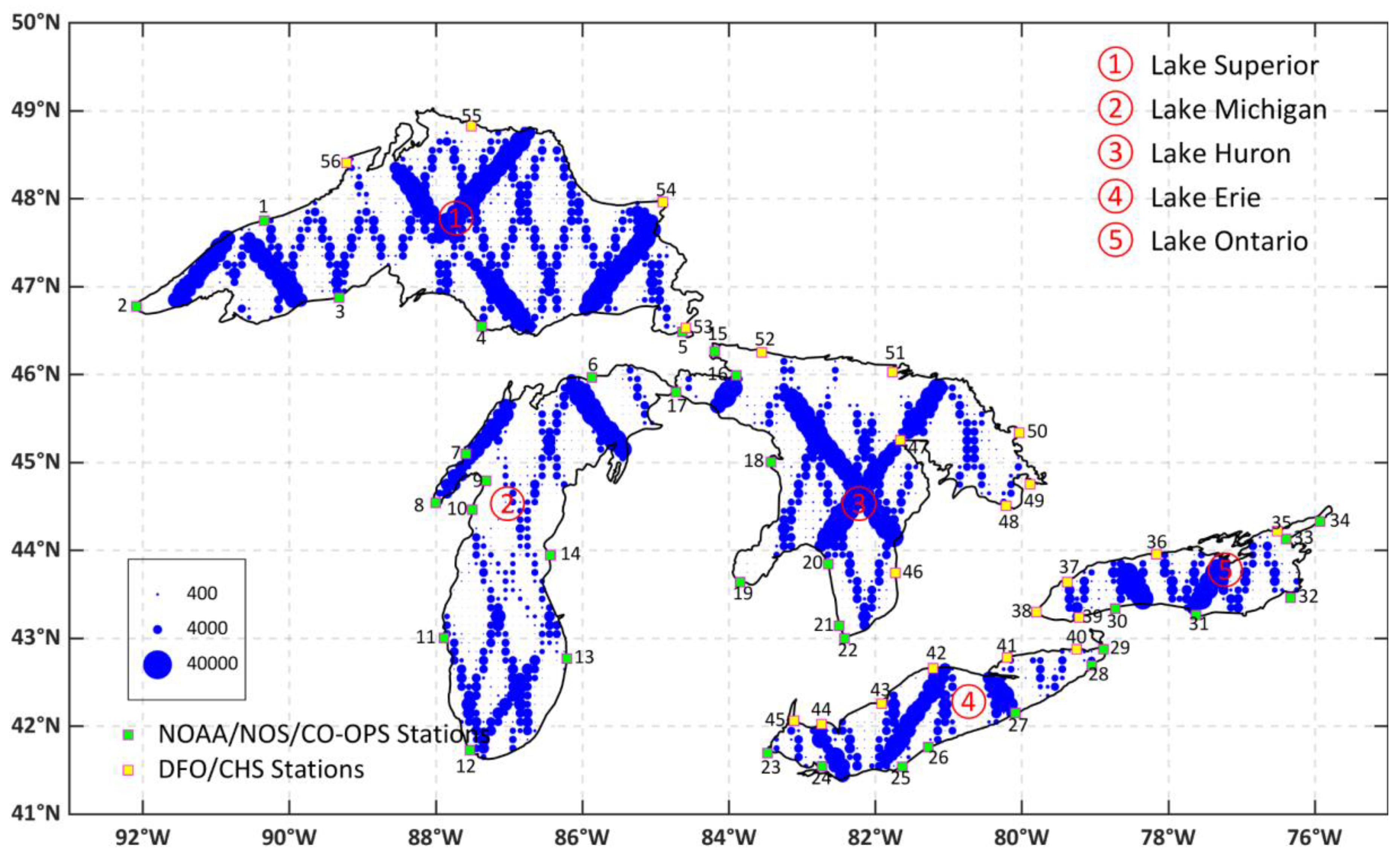
Figure 1. Available altimetry data within ~10 km is shown in blue circles on regular water level maps of the Great Lakes from April 1985 to September 2018. The locations of water level stations are depicted by squares: the green squares show water level stations from NOAA’s Center for Operational Oceanographic Products and Services (NOAA/NOS/CO-OPS), while the yellow squares are stations of the Department of Fisheries and Oceans’ Canadian Hydrographic Service (DFO/CHS).
Remotesensing 14 05194 g001
Figure 2. Temporal coverage of the available altimetry data products used in this study. The datasets start in April 1985 and end in September 2018.
Remotesensing 14 05194 g002
Figure 3. Flow chart describing the main steps of the reconstructed algorithm used in this study.
Remotesensing 14 05194 g003
Figure 4. Rates of (a) radial displacement and (b) geoid change due to GIA in the Great Lakes region. The water level stations used in this study are numbered in (a). The red line in (b) represents the border between USA and Canada.
Remotesensing 14 05194 g004
Figure 5. Time series of lake surface height in each lake of the Great Lakes, reconstructed by EOF (black line), CEOF (blue line), and CICA (red line).
Remotesensing 14 05194 g005
Figure 6. Time series of lake surface height in each lake of the Great Lakes from altimetry data (black line), water level stations (blue line), and CICA reconstruction (red line).
Remotesensing 14 05194 g006
Figure 7. (a) Normalized interannual variations in the Great Lakes. (b) Time series of MEI version 2 from April 1985 to September 2018. (c) Maximum correlation coefficients (95% CI) between the normalized interannual variations and MEI, varying from April 1985 to September 2018. Negative values represent the lake-level variations leading the MEI, and vice versa. (d) Lag months of the maximum correlation coefficients. Here, the first and last 2-year time series were removed to obtain reliable correlation coefficients and lag months.
Remotesensing 14 05194 g007
Figure 8. Interannual variations of lake levels during (a) the 1997–1998 EI Niño; (b) 1998–2000 La Niña; (c) 1987–1988 EI Niño; and (d) 1988–1989 La Niña.
Remotesensing 14 05194 g008
Table 1. Rates of radial displacement and geoid change in the Great Lakes.
GIA EffectsLake SuperiorLake MichiganLake HuronLake ErieLake Ontario
Radial displacement2.02 ± 2.85 mm/year−0.59 ± 1.83 mm/year0.66 ± 2.12 mm/year−2.07 ± 0.31 mm/year−0.36 ± 0.81 mm/year
Geoid change0.12 ± 0.17 mm/year−0.19 ± 0.21 mm/year−0.05 ± 0.17 mm/year−0.32 ± 0.05 mm/year−0.19 ± 0.05 mm/year
Table 2. Correlation coefficient (CC) with 95% confidence intervals (CI) and RMSE viewed as evaluation indicators to compare original altimetry data and reconstructed results.
Great LakesMethodCC (95% CI)RMSE (cm)
Lake SuperiorAltimetry0.9010.80
EOF Rec0.928.69
CEOF Rec0.928.81
CICA Rec0.966.07
Lake MichiganAltimetry0.9314.99
EOF Rec0.988.69
CEOF Rec0.988.42
CICA Rec0.994.89
Lake HuronAltimetry0.9316.45
EOF Rec0.979.49
CEOF Rec0.9710.08
CICA Rec0.979.27
Lake ErieAltimetry0.9013.94
EOF Rec0.9611.17
CEOF Rec0.9611.16
CICA Rec0.977.71
Lake OntarioAltimetry0.8216.52
EOF Rec0.9411.82
CEOF Rec0.9411.26
CICA Rec0.959.89
Table 3. Comparison of averaged radial displacement from ICE-6G, ICE-5G, ICE-4G, ICE-3G, and water level stations, respectively, over the Great Lakes. The data for water level stations’ relative vertical motion is from [8].
Great LakesICE-6GICE-5GICE-4GICE-3GStations
Lake Superior1.751.811.302.301.60
Lake Michigan−0.67−0.940.00−1.40−0.70
Lake Huron0.470.580.902.001.10
Lake Erie−2.19−2.50−0.30−0.600.10
Lake Ontario−0.15−0.310.200.701.40
Publisher’s Note: MDPI stays neutral with regard to jurisdictional claims in published maps and institutional affiliations.