Global Mangrove Extent Change 1996–2020: Global Mangrove Watch Version 3.0

Abstract

Mangroves are a globally important ecosystem that provides a wide range of ecosystem system services, such as carbon capture and storage, coastal protection and fisheries enhancement. Mangroves have significantly reduced in global extent over the last 50 years, primarily as a result of deforestation caused by the expansion of agriculture and aquaculture in coastal environments. However, a limited number of studies have attempted to estimate changes in global mangrove extent, particularly into the 1990s, despite much of the loss in mangrove extent occurring pre-2000. This study has used L-band Synthetic Aperture Radar (SAR) global mosaic datasets from the Japan Aerospace Exploration Agency (JAXA) for 11 epochs from 1996 to 2020 to develop a long-term time-series of global mangrove extent and change. The study used a map-to-image approach to change detection where the baseline map (GMW v2.5) was updated using thresholding and a contextual mangrove change mask. This approach was applied between all image-date pairs producing 10 maps for each epoch, which were summarised to produce the global mangrove time-series. The resulting mangrove extent maps had an estimated accuracy of 87.4% (95th conf. int.: 86.2–88.6%), although the accuracies of the individual gain and loss change classes were lower at 58.1% (52.4–63.9%) and 60.6% (56.1–64.8%), respectively. Sources of error included misregistration in the SAR mosaic datasets, which could only be partially corrected for, but also confusion in fragmented areas of mangroves, such as around aquaculture ponds. Overall, 152,604 km² (133,996–176,910) of mangroves were identified for 1996, with this decreasing by −5245 km² (−13,587–1444) resulting in a total extent of 147,359 km² (127,925–168,895) in 2020, and representing an estimated loss of 3.4% over the 24-year time period. The Global Mangrove Watch Version 3.0 represents the most comprehensive record of global mangrove change achieved to date and is expected to support a wide range of activities, including the ongoing monitoring of the global coastal environment, defining and assessments of progress toward conservation targets, protected area planning and risk assessments of mangrove ecosystems worldwide.

1. Introduction

Understanding the changing extent of mangroves is becoming increasingly critical because of their disproportionate importance in relation to climate, biodiversity and provision of ecosystem services, relative to the small land area that they inhabit. The climate implications of mangrove loss, particularly long-term, include reduced storage of carbon in vegetation and soils [1,2] and reduced capacity to sequester carbon through photosynthesis and trapping of material transported by rivers and coastal currents [3,4]. The resulting changes will have a notable impact on climate change mitigation efforts over short to long-term timeframes [5,6]. As productive and structurally complex ecosystems, mangroves are particularly important as habitats or breeding grounds for fish and invertebrates that support fishers and their communities with nutritional and economic security [7,8]. This same structural complexity also acts as a substantial coastal defence, enabling mangroves to defend shorelines from erosion, reduce flooding, wave impacts and debris movements during storms and, in some locations, to maintain elevation in the face of rising seas [9,10]. Gains in mangrove extent provide the opposite by supporting carbon accumulation and storage, attracting flora and fauna and protecting coastlines against storm impacts and erosion. Protection of mangroves is critical, while the restoration of mangroves has been demonstrated to provide significant ecosystem services benefits over short time periods [4] and is important for reversing at least some of the recent declines in mangrove extent [11].

The environments that replace mangroves depend largely upon whether the drivers of change are natural or anthropogenic [12], but few are able to provide the full range of ecosystem services of natural mangrove ecosystems. Within the world’s intertidal zone, there is a considerable dynamic interplay between mangroves, tidal flats and marshes [13], which are frequently linked to differential responses to processes such as sea level fluctuations, land/sea temperature changes or sediment transport (e.g., [14,15]). More acute or short-term impacts, including cyclones, tsunamis, and lightning strikes, have also resulted in damage to mangroves and promoted transitions to other intertidal ecosystems, which may be temporary or permanent (e.g., [16,17]). Changes in sea level can result in encroachment of mangroves into terrestrial or aquatic ecosystems and vice versa (e.g., [18]). Alongside these processes are many direct human-driven changes that can lead to transitions to other intertidal ecosystem types or to other forms of land-use and land cover, including aquaculture ponds, rice paddies, terrestrial crops, commercial forest plantations, pastoral systems or indeed urban and associated infrastructure. Some human activities can increase mangrove extent, either actively, such as via coastal ecosystem restoration activities [19], or inadvertently through changes in sediment availability [20].

To support global ecosystem monitoring programs, map products must be sufficiently accurate to estimate change, globally consistent, reliable, and repeatedly updated, providing up-to-date and relevant data [21]. Although several global mangrove change products have been developed by other studies, none have been able to achieve all of these broad design principles. Global change estimates are therefore limited by their uncertainties that are typically introduced by merging independently developed products and a lack of a publicly available highly accurate mangrove extent baseline. At the global scale (

Table 1. Comparison of global mangrove change estimates.

Study	Period	Loss (km2)	Annual Loss (km2)	Gain (km2)	Annual Gain (km2)
Hamilton and Casey [22]	2000–2012	1646	137	NA	NA
Goldberg et al. [12]	2000–2016	3363	210	NA	NA
Bunting et al. [25] (GMW v2.0)	1996–2016	4460	223	2273	114
Murray et al. [13]	1999–2019	5561	278	1828	91

), Hamilton and Casey [22] provided the first estimates of global mangrove change using a combination of the Giri et al. [23] mangrove baseline for 2000 and the Hansen et al. [24] forest loss mapping from 2000 to 2012. For the period 2000–2012, Hamilton and Casey [22] estimated that 1646 km² of mangroves were lost. However, only a very limited assessment of the data accuracy was undertaken. Goldberg et al. [12] used Landsat data from 2000 to 2016 and the Giri et al. [23] mangrove baseline to estimate a loss of 3363 km² of mangroves. Bunting et al. [25] (GMW v2.0), while not validated, has been used extensively for mangrove change statistics (e.g., [26]) and uses an earlier version of the methodology and L-band Synthetic Aperture Radar (SAR) data applied in this study. The GMW v2.0 layers estimated 4460 km² of loss and 2273 km² of gain over the period 1996 to 2016, resulting in an estimated net loss of 2187 km². Murray et al. [13] also used Landsat data but for the period 1999–2019, to map changes in tidal wetlands, including mangroves. For mangroves, the loss was estimated at 5561 km² and the gain 1828 km². However, with a focus on tidal wetland change, this study does not develop a mangrove extent baseline and therefore cannot report the magnitude of losses and gains relative to the estimated global extent of mangroves. The most recent effort at mapping mangroves globally has been the Global Mangrove Watch project (GMW; [25,27,28]), where we used radar data from Japan’s Advanced Land Observing Satellite (ALOS) Phased-Array L-band Synthetic Aperture Radar (PALSAR) and optical data from the Landsat Thematic Mapper (TM) to generate a baseline map for 2010. This baseline was subsequently refined using Sentinel-2 imagery, backdated to 2010, to increase the overall accuracy to 95.1% [29], thus creating a reliable and consistent baseline from which change can be detected.

Building on the GMW v2.5 baseline mapping of Bunting et al. [29], the aim of this study was to establish the magnitude of change in mangrove extent at the global scale to inform overall trends from the mid-1990s to the present. This study provides the longest time period over which change in mangrove extent has been assessed on a global scale. The main objectives were to:

1.

Establish a change detection approach to map mangrove extent for multiple years (1996, 2007–2010, and annually from 2015 to 2020) based on the available L-band SAR data.

2.

Develop a method for estimating the uncertainty of the mapped extent and changes between years.

3.

Identify at a global level, but with consideration given to regional variations, the main areas where losses and gains are evident and provide a reference dataset for mangrove extent and change suitable for global and national-level reporting.

The products from the study were developed for integration within the Global Mangrove Watch Platform [26]. However, they can also provide important data to national systems for forest and/or wetlands monitoring, to national inventories and reporting processes for international agreements and conventions, as well as for regional to local monitoring of mangrove change. The existing GMW v2.0 dataset [25] was developed to support a number of international agreements and conventions, in particular the Ramsar Convention on Wetlands of International Importance and the UNFCCC Paris Agreement. It is currently used for reporting on the UN Sustainable Development Goals [30], as well as for conservation action (e.g., by non-governmental organizations; NGOs). We expect the GMW v3.0 to continue to be used to support reporting on these international agreements and conventions. The importance of mangroves has also recently been highlighted by the Convention on Biological Diversity (CBD) and the Intergovernmental Panel on Climate Change (IPCC).

2. Methods

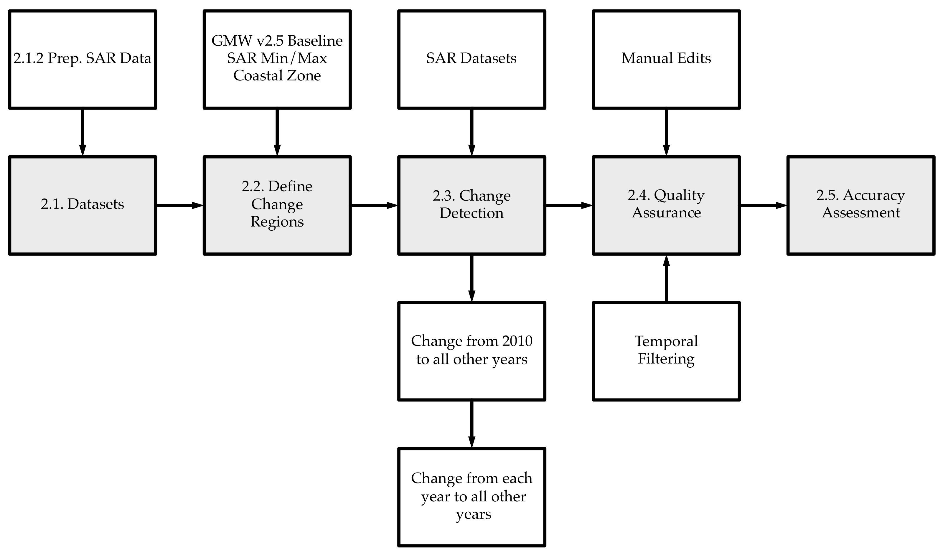
This study builds on the 2010 global mangrove baseline map, GMW v2.5, Bunting et al. [29], in which L-band SAR data from the JERS-1 (1996), ALOS (2007–2010), and ALOS-2 (2015–) missions of the Japan Aerospace Exploration Agency (JAXA) were used to perform change detection from the 2010 baseline to generate mangrove extent maps for the years 1996, 2007, 2008, 2009, 2010, 2015, 2016, 2017, 2018, 2019 and 2020. The analysis was undertaken on the SuperComputing Wales (SCW) High-Performance Computing (HPC) infrastructure using the Remote Sensing and GIS Library (RSGISLib) of tools [31], the KEA image format [32] and the pbprocesstools [33] workload library to manage the workflow of tasks on the HPC. The overall workflow is illustrated in Figure 1 and detailed below.

2.1. Datasets

2.1.1. 2010 Mangrove Baseline

The GMW v2.5 mangrove baseline [29] was used for this study and it constitutes the most spatially complete and accurate global mangrove extent dataset currently available [29]. The GMW v2.5 baseline was developed and refined over four generations and is spatially aligned with the 2010 ALOS PALSAR global data mosaic [34]. The 2010 GMW v2.5 baseline map suggests that the global extent of mangroves in 2010 was 140,260 km${}^2$. The baseline has a map accuracy of 95.1% with a 95th confidence interval of 93.8–96.5%. Nevertheless, within the GMW v2.5 analysis, some regions were found to be missing, particularly within eastern India, western Africa and the Pacific. These areas were added to the baseline using the methodology of Bunting et al. [29].

2.1.2. L-Band Synthetic Aperture Radar (SAR)

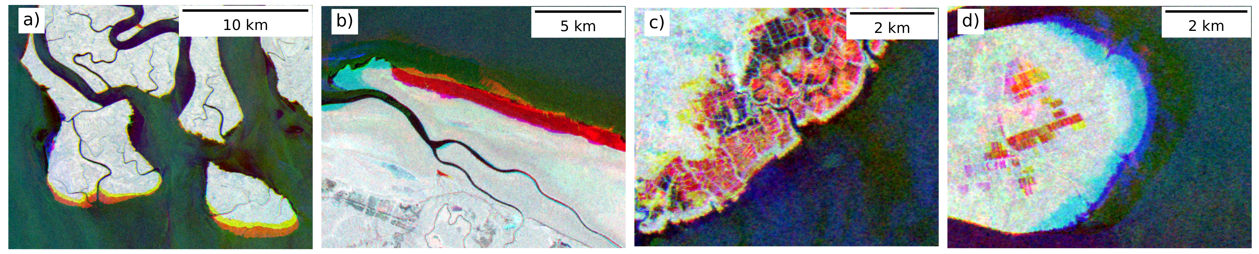
This study builds on the work of Thomas et al. [35,36,37] which demonstrated that long wavelength (L-band, 23.5 cm) SAR data are sensitive to mangrove change and useful for detecting both mangrove gain and loss (Figure 2). An advantage of using SAR is that microwaves provide observations regardless of illumination and weather conditions, overcoming a widely reported limitation of optical systems (e.g., Landsat and Sentinel-2), and enabling observations in regions where persistent cloud cover reduces useable observations, such as along tropical and sub-tropical coastlines.

The L-band SAR data used as the basis for this analysis were acquired by the JERS-1 SAR, ALOS PALSAR and ALOS-2 PALSAR-2 sensors and made available by JAXA as public open global mosaic products (JAXA version release 1). The ALOS and ALOS-2 mosaics were provided as dual-polarisation (HH and HV) radar backscatter, while the JERS-1 mosaic was available in HH-polarisation only. The mosaics were provided as $1\times 1$ degree tiles, at 25 m (0.8 arc seconds) pixel spacing, covering 11 annual epochs between 1996 and 2020 (

Table 2. The time periods for the JAXA L-band SAR mosaic dataset.

Sensor	Years	Mosaic Version
JERS-1 SAR	1996	v1(C)
ALOS PALSAR	2007, 2008, 2009, 2010	v1(O)
ALOS-2 PALSAR-2	2015, 2016, 2017, 2018, 2019, 2020	v1(K)

).

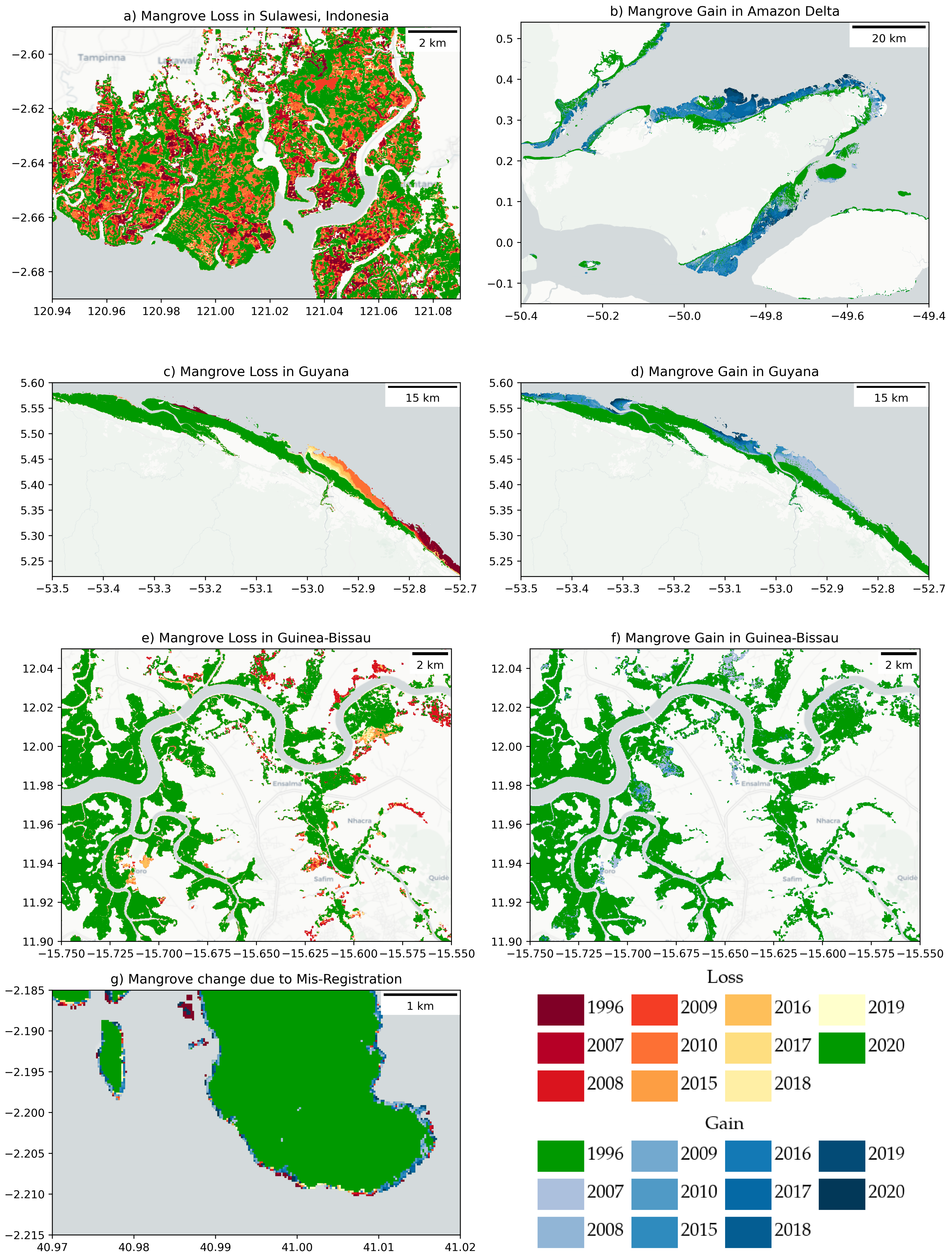
Initial efforts to develop the change analysis revealed some misregistration between the different years of the SAR mosaics, resulting in the omission of known change events and commissions where change was known not to have occurred. This was particularly evident in the mosaics constructed from the JERS-1 SAR data from 1996. In these mosaics, a significant non-linear shift from the 2010 ALOS PALSAR mosaic, typically ranging from 1 to $>5$ pixels, was observed due to an error within JAXA’s standard mosaic processing pipeline. To reduce the impact of this misregistration, tie points were automatically generated using the method of Bunting et al. [38] using the ALOS PALSAR 2010 mosaic as the reference dataset. Tie points were created on a single 100-pixel grid using a 100-pixel window around each tie point to locate the image shift using the maximum correlation between the two images within the window. A visual check of the tie points was conducted to identify and remove those that were incorrectly matched (e.g., due to true change). A thin-plated spline transformation and a nearest neighbour interpolation, implemented within the GDAL software, were then used to warp the JERS-1 SAR data.

The ALOS PALSAR (for all years other than 2010) and ALOS-2 PALSAR-2 from 2015 to 2017 were found to be generally well registered but with a non-linear shift of about ±1 pixel when compared to the 2010 ALOS PALSAR mosaic. For ALOS-2 PALSAR-2 mosaic products from 2017 to 2020, JAXA improved the absolute spatial registration by enhancing the data processing system. However, this resulted in an increased spatial misregistration with the 2010 mosaic by up to ±4 pixels for 2019 and 2020. For this reason, a further image-to-image registration step was undertaken where an overlap of 50 pixels was added to each of the 2007–2020 mosaic tiles, which were moved by ±5 pixels in the $x/y$ axes until the correlation between the tile for each year and for 2010 reached a maximum. A sub-pixel component of the offset was then estimated using the method outlined in Bunting et al. [38] and the tile was then shifted by this amount and the overlapping regions removed. Following this registration process, the individual mosaic tiles were found to be <±1 pixel to the 2010 mosaics.

The remaining misregistrations were found to be non-linear and locally variable. Whilst further tie points could have been generated to correct these errors, full automatisation of this process is challenging and also likely to introduce further errors where tie points are mis-located, particularly around areas of change.

Of the JAXA datasets, the 2019 and 2020 ALOS-2 PALSAR-2 data were most accurate in terms of absolute registration, aligning very well with Sentinel-2, Landsat and other image datasets. On this basis, and globally, the average absolute misregistration with the GMW 2010 baseline was determined to be less than 100 m, which should to be considered when used in analyses with other spatial datasets. Due to the dependence on the 2010 GMW v2.5 mangrove baseline, all other datasets were geometrically aligned to the 2010 dataset.

2.1.3. Other Datasets

In addition to the JAXA SAR mosaic data, several other datasets were used to develop and refine the 2010 mangrove contextual change mask (Section 2.2). The datasets included the Shuttle Radar Topographic Mission (SRTM) elevation data, the General Bathymetric Chart of the Oceans (GEBCO; 15 arc-second intervals [39]), the Global Surface Water product [40] and the Database of Global Administrative Areas (GADM) Version 3.6.

2.2. Defining Change Regions

As described by Bunting et al. [27,29], the ability to separate mangroves from other proximal land covers using L-band SAR data alone is limited. Therefore, optical (Landsat and Sentinel-2) data were used in conjunction with the ALOS PALSAR mosaic to support the generation of the 2010 GMW mangrove baseline map. The L-band backscatter at both HH and HV polarisations is sensitive to the amount, moisture content and geometry of the woody components of the mangroves, which often are affected when changes (e.g., deforestation, degradation or growth) occur [35,36,37]. As such, differences in L-band data between observations can be used to inform on changes in the extent and, to a lesser degree, the condition of mangroves (e.g., Figure 2). Where pixels are classified as mangroves in the 2010 GMW baseline but not for another date within the time-series, then the detection of change is relatively straightforward, as only the pixels within the 2010 mangrove mask will be considered. However, for pixels that were not mangroves in 2010 but mangroves in another year, identifying pixels where change might have occurred is more challenging and requires a contextual definition. Such an approach enables the exclusion of many pixels that could not be mangrove being incorrectly associated with change to mangroves.

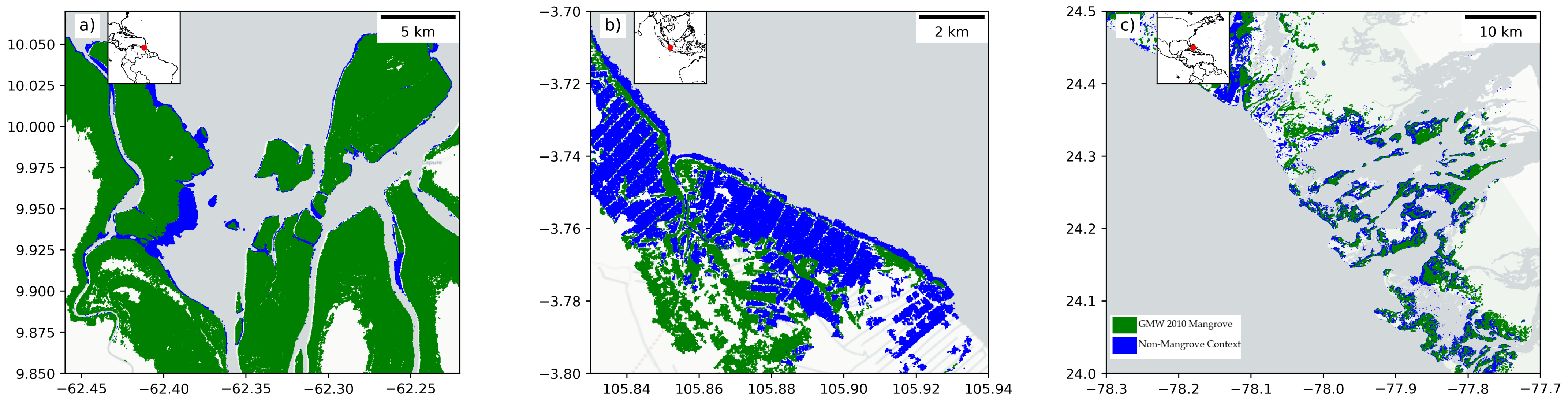
When visually examining the time series imagery (e.g., Figure 2), the human brain is very good at contextually filtering the data to identify likely mangrove changes. Unfortunately, current automated computational approaches do not have the same ability to classify context. Therefore, to make best use of the L-band SAR data, a contextual layer for changes outside the 2010 mangrove baseline needed to be defined (e.g., Figure 3). This layer was similar to the low backscatter surface in Bunting et al. [29] but was relevant to the whole time-series rather than just 2010.

To define the potential change regions outside of the 2010 mangrove baseline (i.e., the contextual layer), a coastal zone that encompassed areas within 2.5 km of the GADM coastal boundary and within 500 m of the GMW 2010 baseline while excluding those with a terrestrial surface elevation higher than 20 m or a bathymetric depth lower than −100 m, was used. Within this coastal zone, the differences between the maximum and minimum backscatter at each HH and HV polarisation were calculated to identify regions most likely to have experienced change, with these based on areas where (a) the difference threshold for L-HV was >8 dB, the minimum L-HV was <−18 dB and the maximum L-HV was >−25 dB or (b) where the 0 > JERS-1 L-HH >−11 dB and the minimum HV was <−18 dB. These thresholds were defined through visual interpretation of reference sites distributed globally.

Within this potential change area, mangroves were associated with a high L-band backscatter and non-mangrove areas (e.g., water, mudflats, salt marshes) had a low backscatter. Changes in backscatter were assumed to represent a steady transition or abrupt change between these categories. The ability to detect such changes depends on the time separation between the observations as some natural processes (e.g., sea level fluctuation) or events (e.g., strong winds, floods) or human activities (e.g., the establishment of plantations or construction of new port facilities) might be mistaken for changes in mangroves if observations are several years or decades apart. This is particularly the case if the land cover at the observation time exhibits a backscatter signal similar to the mangrove or non-mangrove states. However, the extent of confusion was expected to be low, particularly as manual inspection and editing of the contextual mask had been undertaken a priori. The manual inspection involved the digitisation of regions which should be removed from the mask (i.e., incorrectly included within the mask) and additions to the mask (i.e., regions where mangroves could occur but were not included within the mask). Any pixels which were permanently water during the period were masked using the water ’occurrence change intensity’ layer 1984–2020 from Pekel et al. [40], where pixels which were water in both periods were removed from the potential mangrove change layer. In addition, regions of mangrove change from Bunting et al. [25] and Goldberg et al. [12] were included in the potential change area and, based on visual interpretation, regions known not to be mangrove change or otherwise were manually removed or added. Examples of this contextual potential change layer are shown alongside the 2010 GMW v2.5 baseline in Figure 3.

2.3. Change Detection

A map-to-image method was used for the change detection, with an approach based on Thomas et al. [37]. The map-to-image approach aims to update the baseline map using an input SAR image rather than reclassifying the input imagery or directly comparing imagery from multiple dates. Only the two classes, mangrove and non-mangrove, were analysed for this analysis.

The mangrove class was initially defined using the 2010 GMW v2.5 baseline and the non-mangrove regions by the change regions defined in the previous step. From this baseline, a mangrove/non-mangrove map, where the non-mangrove regions was defined using the context mask, was produced for each of the change years (1996–2020), with each representing a unique baseline. The change analysis was then applied from each year to all the other years, including 2010, generating 10 change maps for each year. The final overall maps were then created for each year based on the classification majority (i.e., a pixel has be identified as mangroves >5 times). This analysis was conducted on a per-pixel basis where, within the mangrove/non-mangrove masks, a threshold of the L-band SAR data was defined by splitting the change pixels from the original class. For the ALOS PALSAR and ALOS-2 PALSAR-2 data (2007–2020), the threshold was defined using the HV polarisation as this was found to be more consistent with less direct scattering from the water surface, which otherwise can produce false positives for change during certain surface conditions. However, for the single-polarisation JERS-1 SAR (1996) data, the threshold had to be defined using the HH polarisation.

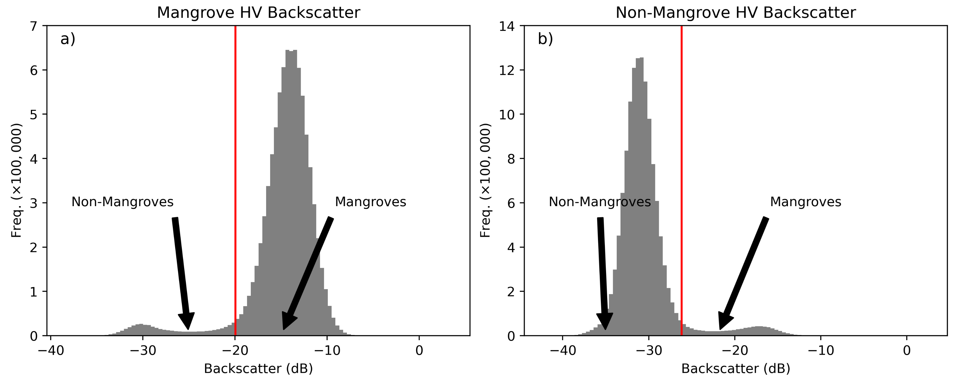
Two key assumptions of the map-to-image approach to change detection are that change occurs rarely and that the response within the remote sensing imagery (i.e., SAR backscatter) will be altered, resulting in a difference in the digital number (DN) values for pixels where a change has occurred compared to those where no change has taken place. When visualised as a histogram (Figure 4), the DN values of the change pixels will form a tail to the histogram (i.e., outliers) and hence threshold identification can make use of the many outlier identification algorithms available (e.g., [41]). For this, the thresholding method proposed by Thomas et al. [37] was used, where the class response is assumed to be normal (Figure 5) and the threshold that separates outliers (and hence identifies the change within mangrove and non-mangroves classes) is derived by optimising the skewness and kurtosis splitting the histogram (e.g., Figure 4).

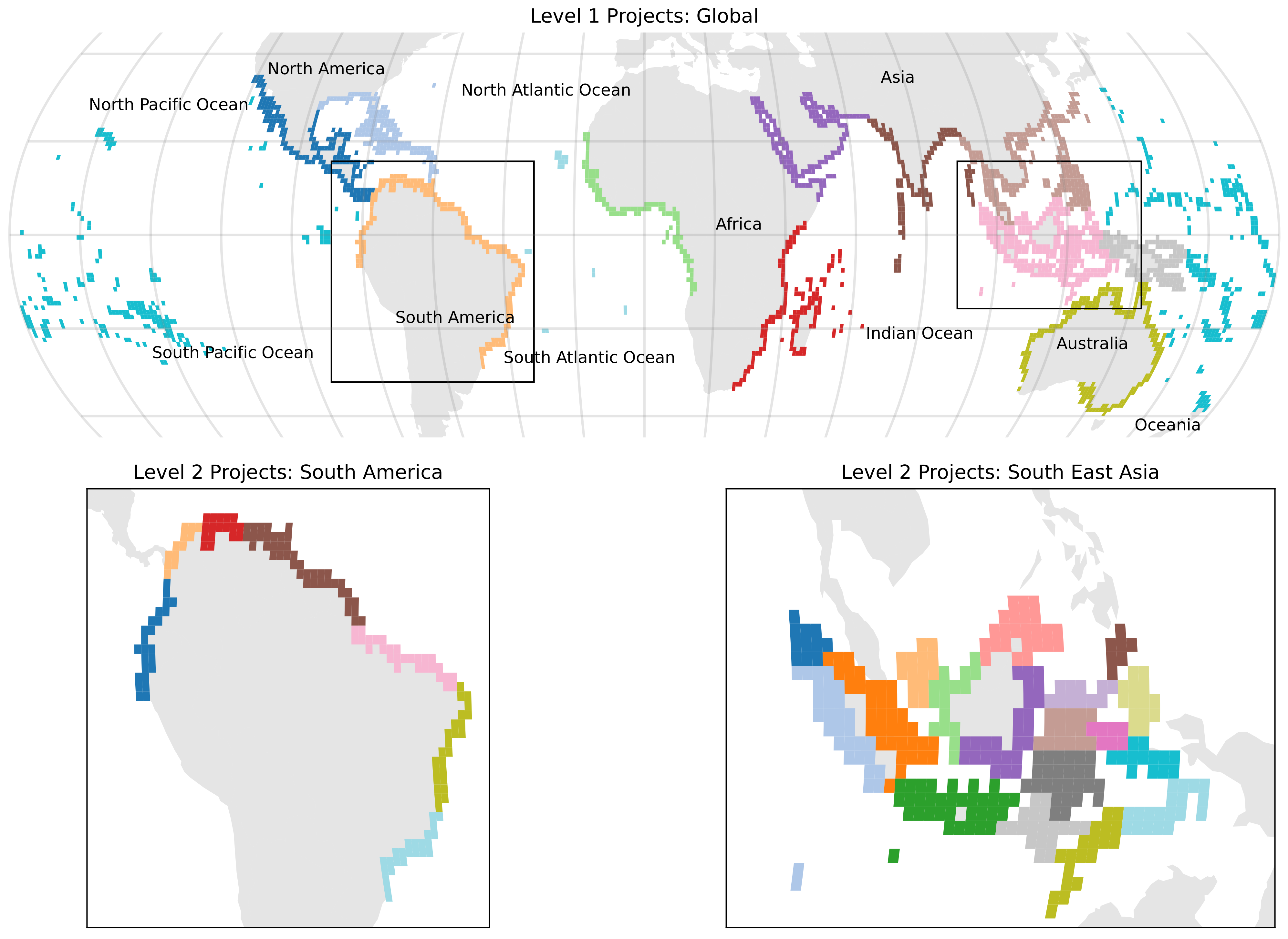
Given that change is rare, identifying thresholds on a $1\times 1$ degree tile basis would result in situations where there are no changes or only small areas of mangroves are within the tile (e.g., tile edges or islands). Therefore, either an incorrect threshold or no threshold might be identified. To identify the change thresholds the project extents defined by Bunting et al. [27] (Figure 6), merging neighbouring $1\times 1$ degree tiles into connected regions, were revised and used.

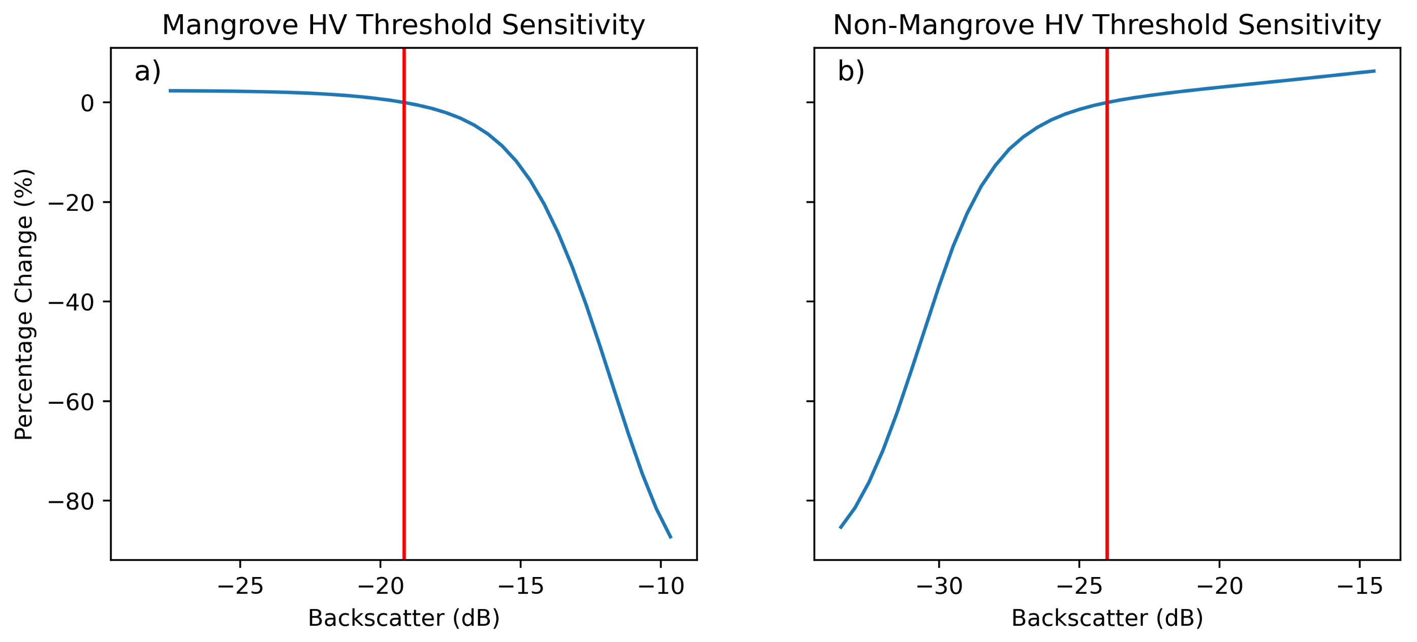
Thresholds were first calculated from the 2010 baseline for both classes and L-band polarisations (HH and HV) to all the years and filtered prior to application to the SAR data. This was achieved by calculating the median threshold across all years (2010 to other years) on a per-project basis. For years where the threshold was >2 dB from the median, the median value was substituted to ensure that changes were not artefacts within the time-series that resulted from strong variability in the thresholds. The mean and standard deviation of the thresholds, using all years as the baseline, are shown in

Table 3. The average and standard deviations of the thresholds used to separate mangroves and non-mangroves changes.

Year	Mangrove to Non-Mangrove	Non-Mangrove to Mangrove
1996 (HH)	−14.03 (1.84)	−14.38 (3.26)
2007 (HV)	−20.23 (2.05)	−24.34 (1.01)
2008 (HV)	−20.21 (2.03)	−24.31 (1.06)
2009 (HV)	−20.27 (2.00)	−24.29 (1.02)
2010 (HV)	−20.24 (2.00)	−24.26 (1.12)
2015 (HV)	−20.87 (2.17)	−24.50 (1.31)
2016 (HV)	−20.85 (2.14)	−24.57 (1.28)
2017 (HV)	−20.86 (2.16)	−24.68 (1.29)
2018 (HV)	−20.62 (2.16)	−24.80 (1.35)
2019 (HV)	−20.85 (2.33)	−25.14 (1.44)
2020 (HV)	−20.89 (2.34)	−25.12 (1.50)

. As expected, the thresholds are consistent throughout the time series with some variation between areas (projects) due to site variations. Site variations mainly occur due to the size of the mangrove. For example, in areas such as Indonesia, mangroves are typically over 12 m in height while in China they are less than 5 m in height [42]. The backscatter thresholds used for the 1996 JERS-1 data were higher given the use of the HH rather than HV polarisation.

A sensitivity analysis was conducted to quantify the differences in the mangrove area mapped given the variation in the thresholds. The sensitivity analysis demonstrated that changes in the thresholds of <2 dB resulted in only small changes in the area of mangroves, with these being <2% (Figure 7).

2.4. Quality Assurance

The quality assurance (QA) processing step (Figure 1) sought to improve overall map accuracy through the application of several standard data post-processing procedures. The QA was only applied to the final mangrove extent layers and consisted of two temporal filters alongside manual edits created through visual assessment of the data layers. The first temporal filter ensured the time series of mangrove maps were temporally consistent, preventing pixels from switching back and forth between mangroves and non-mangroves. For example, if a pixel was mangroves in 2007, non-mangroves in 2008 and mangroves in 2009, then the 2008 classification would be reverted to mangroves. An extensive visual assessment of the dataset was conducted where pixels mapped as mangroves but visually identified as having not been mangroves at any date within the time series were removed from the dataset. Additionally, a few small areas were found to be mangroves across the entire time series but were missing from all years and these were therefore added to the mangrove mask in all years. Edits were not applied independently to individual years as the time to generate such inputs would be significant.

Finally, a number of small change features (i.e., mangrove gain or loss) were observed that were either 1 or 2 pixels in size, with many associated with the residual misregistration between the input L-Band SAR data. Therefore, the time series was sequentially filtered from 1996 such that change features between the consecutive years of 1 or 2 pixels in size were removed (i.e., not changed) on the condition that the relative border of the change feature was <0.5 with the class being changed to. For example, if a feature consisting of two pixels changed from non-mangroves to mangroves, it would be accepted as a change if the relative border to mangroves was ≥0.5.

2.5. Accuracy Assessment

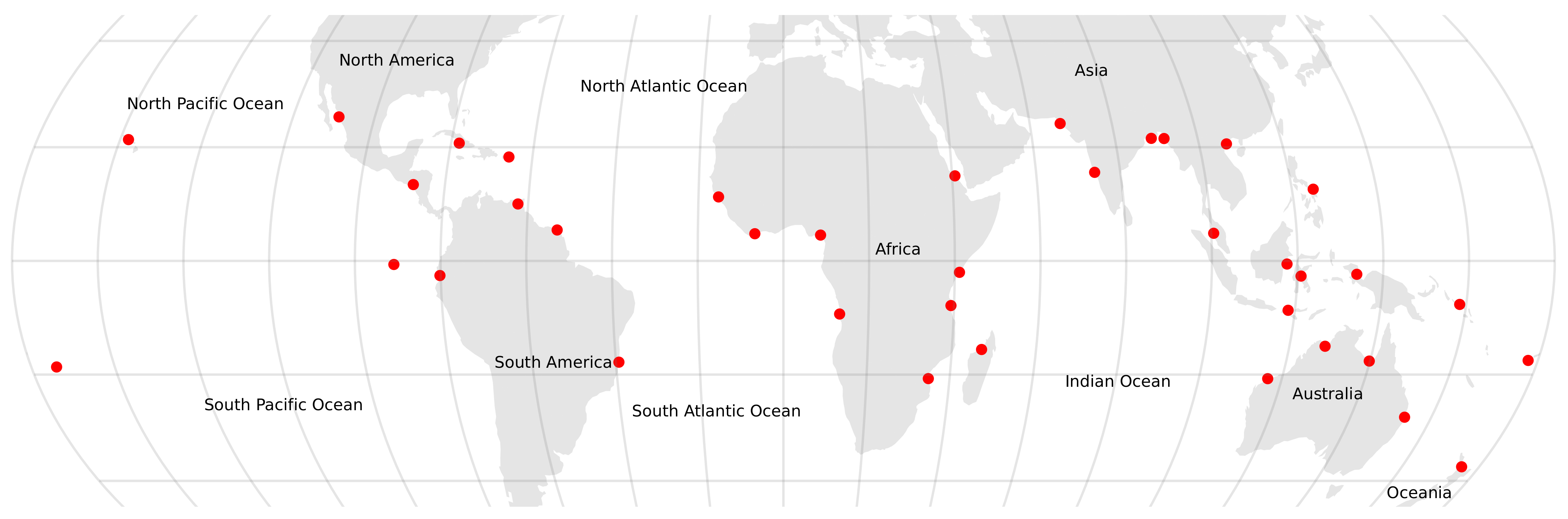
The accuracy assessment was undertaken in two parts. The first used the 60 validation sites from Bunting et al. [29] for 2010 to compare the accuracies of the GMW v3.0 2010 mangrove extent with the GMW v2.5 2010 baseline. This provided an assessment of the impact the SAR change detection processing had on the quality of the mapped mangrove extent. The second assessment focused on the accuracy of the change detection. This assessment defined a new set of 38 sites (Figure 8) covering a diverse range of geographic regions, mangroves types and change drivers that were considered to represent the full range of known and expected change events globally and included areas without changes. For each site, a $0.2\times 0.2$ degree reference area was located such that it overlapped with as much of the mangrove area as possible and usable historical Landsat imagery was available for multiple dates as an independent reference for mapped changes. The advantage of using Landsat data over other available historical optical datasets are that the inclusion of shortwave infrared channels allowed mangroves to be more easily distinguished and data were freely available for each site. The Landsat data (Collection-1 product) was accessed via the Google Earth Engine, with median composites of non-cloud pixels created using all the images acquired within the year of interest.

For assessing the accuracy of change detection, four change classes were considered (

Table 4. Definitions of the change classes.

Class	Description
Mangroves	Mangrove in both observations.
Non-Mangroves	Not mangroves in both observations.
Mangroves > Non-Mangroves (Loss)	Mangroves at the earlier observation and not mangroves at the later observation; i.e., a loss of mangroves.
Non-Mangroves > Mangroves (Gain)	Not mangroves at the earlier observation and mangroves at the later observation; i.e., a gain of mangroves.

), representing no change (mangroves, non-mangrove), mangrove gain and mangrove loss. Given the relative areas of the four classes within the classifications, identifying sufficient reference points for the change classes was challenging, particularly considering change omissions. Therefore, two sampling methods for defining reference points were used for each of the 38 sites.

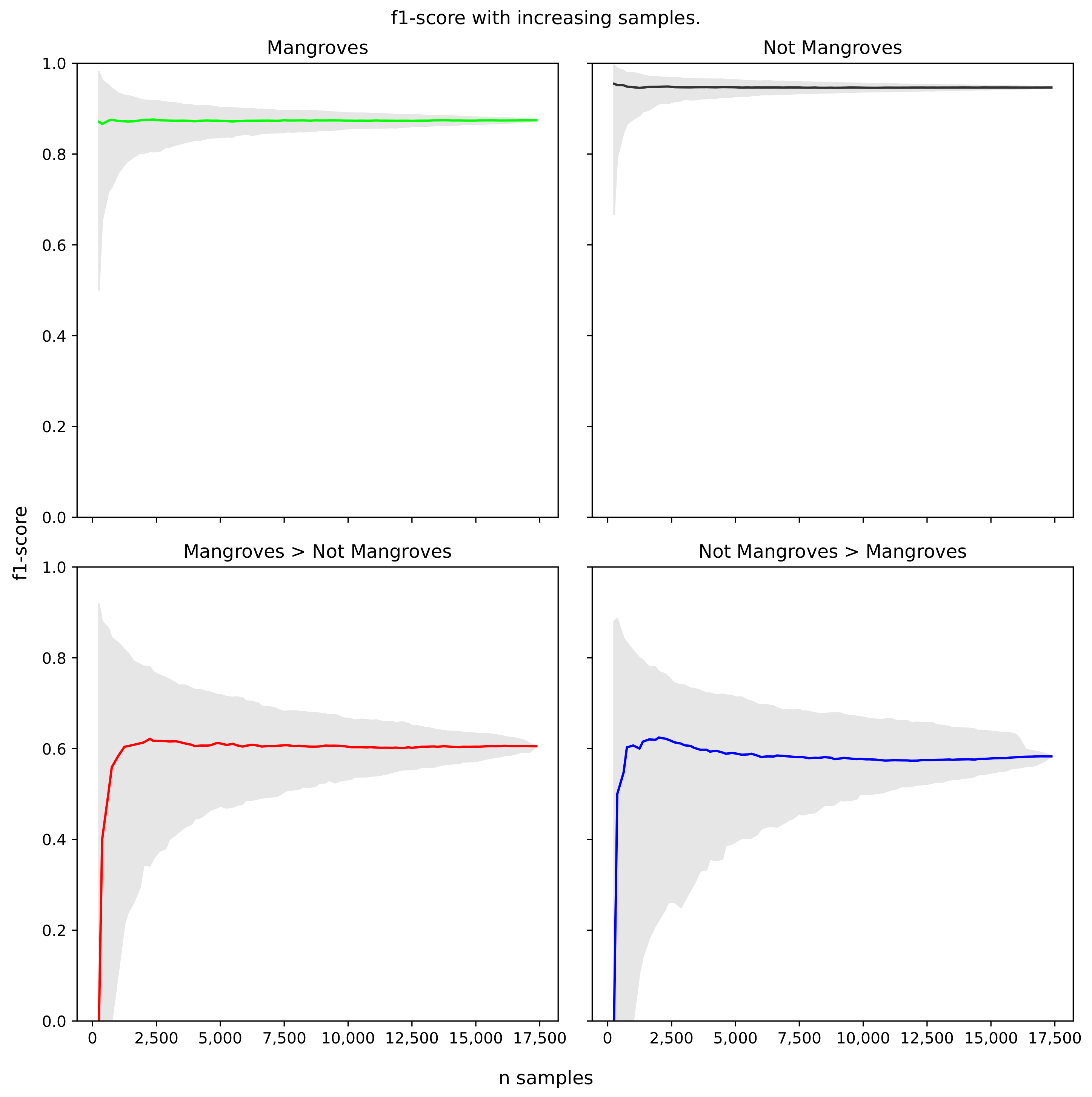
For the first, 500 points were distributed randomly within each $0.2\times 0.2$ area for a pair of randomly sampled years, with the condition that the base year had to be earlier than the change year. These points were not stratified for particular classes or temporal periods as sampling was proportional to the area mapped for each class and the temporal period was randomly selected. The number of change samples (’mangroves > non-mangroves’ = 139, ’non-mangroves > mangroves’ = 39) identified was naturally small, as these are globally rare. Therefore a second set of points was defined within regions where changes were known to have occurred (determined through manual annotations) or defined as change by the change analysis. The temporal period was also maximised using the earliest and latest year for which useable Landsat reference imagery were available. Within these change regions, further reference points (up to 500) were defined through random selection of pixels, where if the number of change pixels was ≤500 then half the available pixels were selected. By focusing the second set of points on the change regions, a sufficient number of reference change points was realised in a manageable amount of effort. The reference points were manually annotated with a reference class based on an informed interpretation of the Landsat imagery. Each of the 76 points sets (38 sites × 2 sampling methods) were then split into two (i.e., two sets of 250 points), where the first set were annotated with their reference class and the second set were randomly selected and annotated until sufficient points had been assessed. Sufficient points were deemed to have been annotated once the addition of new reference points did not significantly change the F1-scores of the change classes (see Section 3.3). This resulted in 11,769 non-mangroves, 4482 mangroves, 702 ’Mangroves > Non-Mangroves’ and 413 ’Non-Mangroves > Mangroves’ points being sampled. Therefore, the complete validation set had 17,366 reference points.

2.6. Addressing Uncertainty

Reporting the uncertainty of a map with confidence intervals around derived estimates is important to enable data end-users to understand map limitations, propagate known uncertainties and characterise the performance of mapping protocols. Unfortunately, transparently reporting map accuracy and propagating error via confidence intervals is commonly not undertaken. Using the bootstrapping method of Murray et al. [13,43] 95th confidence intervals for the accuracy statistics and mangrove extent and change areas were calculated. For the bootstrap, 1000 iterations using a 40% sample of the validation set (i.e., 6946 reference points), with replacement, were used to estimate the variance of the accuracy statistics. The 95th confidence interval was defined using the 5th and 95th percentiles of each of the resulting accuracy statistics.

To calculate the area based confidence interval for both the mangrove extent and gain and loss maps the 95th confidence intervals of the class (e.g., mangroves; Section 3.3) omission and commission were calculated and these were used to calculate the extent confidence interval of each class:

$$\begin{array}{c}\hfill {\mathrm{area}}_{i}95{\mathrm{CI}}_{\mathrm{Lower}}={\mathrm{area}}_i-({\mathrm{area}}_i\times \mathrm{commission}{\mathrm{P}}_{95})\end{array}$$

(1)

$$\begin{array}{c}\hfill {\mathrm{area}}_{i}95{\mathrm{CI}}_{\mathrm{Upper}}={\mathrm{area}}_i+({\mathrm{area}}_i\times \mathrm{omission}{\mathrm{P}}_{95})\end{array}$$

(2)

A single accuracy assessment was conducted for the four classes in Table 4, which includes the gain and loss classes. Therefore, the same approach is applied to both the mangrove class, and the gain and loss classes. As a single estimate of commission and omission was produced for all years these are constant across all years of the time series.

2.7. Adjustment of Change Area

Using the omission and commission statistics from the accuracy assessment, the mapped area estimates for the mangrove extent and gains and losses were adjusted to reflect the impact of known sources of map error [44,45]. Known sources of map commission and omission errors included the residual misregistration between the observations.

To calculate the adjusted area (${\mathrm{area}}_a$) for the gain (g) and loss (l) classes, the omission and commission errors are estimated from the error matrix (see Section 3.3) and used with the mapped areas (${\mathrm{area}}_m$) as follows:

$$\begin{array}{c}\hfill {\mathrm{area}}_{ag}={\mathrm{area}}_{mg}-({\mathrm{area}}_{mg}\times {\mathrm{commission}}_g)+({\mathrm{area}}_{mg}\times {\mathrm{omission}}_g)\end{array}$$

(3)

$$\begin{array}{c}\hfill {\mathrm{area}}_{al}={\mathrm{area}}_{ml}-({\mathrm{area}}_{ml}\times {\mathrm{commission}}_l)+({\mathrm{area}}_{ml}\times {\mathrm{omission}}_l)\end{array}$$

(4)

Note, the estimated omission and commission errors should have a range 0–1. To calculate the total adjusted mangrove extents, the adjusted gain and loss areas from 1996 for each year were added to the 1996 mangrove extent area.

3. Results

The results of the analysis demonstrate the ability of the GMW v3.0 product to map mangrove change through time (Figure 9a–f). The GMW v3.0 datasets are able to identify many causes of change, but the most commonly observed are losses due to coastal erosion (Figure 9c) and deforestation (Figure 9a), and gains due to sedimentation around river estuaries (Figure 9b). However, we also observed that the remaining misregistration of the input JAXA L-band SAR data resulted in some commission and omission errors (e.g., Figure 9g which illustrates a region heavily impacted by the error), which are individually small in area but add uncertainty to the change estimates. Given the random nature of the input data misregistration errors, the changes associated with errors are considered to be similar in terms of gain and loss. Therefore, the observed net change rather than independent gain and loss statistics from this analysis are recommended to be used.

3.1. Global Mangrove Change

Globally, our map datasets suggest that a net 3.4% (5245 km²) of mangrove extent has been lost between 1996 and 2020 (

Table 5. Global mangrove extent estimates 1996–2020 and change since 1996 in km². Note: reported mangrove extent estimates account for known map commission and omission errors.

Year	Extent	95th Conf. Int.	Change Since 1996	% Change Since 1996
1996	152,604	133,996–176,910	-	-
2007	149,973	130,949–172,887	−2631	−1.7%
2008	148,645	129,419–170,868	−3959	−2.6%
2009	148,453	129,197–170,575	−4151	−2.7%
2010	148,020	128,709–169,930	−4584	−3.0%
2015	147,345	127,940–168,915	−5260	−3.4%
2016	147,070	127,624–168,497	−5535	−3.6%
2017	147,260	127,832–168,772	−5344	−3.5%
2018	147,554	128,155–169,199	−5050	−3.3%
2019	147,605	128,206–169,266	−4999	−3.3%
2020	147,359	127,925–168,895	−5245	−3.4%

), with a rate of loss approximately twice that of gain. As mangroves are naturally dynamic systems changes have occurred in almost all parts of the world. However, hotspots of mangrove change are clearly present in a number of locations (Figure 10). Significant losses are commonly associated with two main drivers, coastal erosion or anthropogenic deforestation. While significant gains are commonly associated with a supply of new sediments, typically at the mouths of large river systems (e.g., the Amazon; Figure 9b).

3.2. Regional Mangrove Change

Table 6. Mangrove extent estimates 1996–2020 for the UN Statistics geographic regions in km². Individual country statistics are within Appendix A. Note: reported mangrove extent estimates account for known map commission and omission errors.

UN Region	UN Sub-Region	1996	2007	2008	2009	2010	2015	2016	2017	2018	2019	2020
Africa	Eastern Africa	7883.3	7789.0	7713.6	7702.1	7688.6	7678.9	7661.5	7670.1	7683.4	7669.9	7610.0
	Middle Africa	4531.3	4533.2	4527.8	4530.8	4530.5	4530.4	4517.6	4515.7	4514.5	4520.8	4514.0
	Southern Africa	25.7	26.2	26.0	26.0	26.1	26.4	26.3	26.4	26.5	26.6	26.4
	Western Africa	17,558.5	17,504.8	17,409.2	17,415.7	17,400.1	17,375.1	17,298.0	17,296.0	17,290.1	17,272.2	17,200.8
Americas	Caribbean	6545.1	6260.1	6136.1	6133.0	6057.5	5960.0	5936.0	5957.7	5984.0	6007.4	6031.3
	Central America	15,003.3	14,789.1	14,660.3	14,589.4	14,547.7	14,461.2	14,450.1	14,503.0	14,597.6	14,586.4	14,466.3
	Northern America	2400.1	2388.8	2371.3	2371.5	2342.2	2307.1	2297.5	2296.4	2303.1	2319.0	2329.3
	South America	20,516.5	20,273.5	20,209.7	20,218.8	20,205.1	20,199.9	20,251.3	20,331.5	20,376.5	20,395.0	20,378.1
Asia	Eastern Asia	257.2	237.3	231.3	226.0	223.6	228.0	232.1	232.8	230.1	229.8	227.7
	Southeastern Asia	50,678.8	49,254.2	48,663.8	48,572.3	48,440.9	48,115.5	47,965.1	47,952.7	47,983.2	48,046.4	48,222.3
	Southern Asia	9960.7	9846.3	9759.9	9737.3	9710.4	9733.6	9774.1	9791.6	9829.1	9777.1	9661.1
	Western Asia	201.5	214.5	218.0	213.2	193.5	174.5	170.9	172.7	173.3	173.7	173.6
Oceania	Australia & New Zealand	10,945.0	10,752.2	10,618.0	10,618.3	10,562.5	10,478.4	10,425.5	10,451.7	10,497.3	10,517.9	10,466.9
	Melanesia	5932.8	5941.3	5937.8	5936.8	5927.2	5910.6	5898.4	5896.5	5900.2	5900.7	5889.4
	Micronesia	149.8	147.4	147.4	147.2	149.5	150.0	150.0	150.3	150.4	147.5	147.1
	Polynesia	14.9	14.8	14.8	15.0	15.0	15.1	15.1	15.0	14.9	14.9	14.7
Global		152,604	149,973	148,645	148,453	148,020	147,345	147,070	147,260	147,554	147,605	147,359

summaries mangrove change at regional levels using the UN Statistics Geographic Regions [46], while country level statistics have been provided in Appendix A. The largest area of mangroves is located within Southeast Asia, and this region has experienced the largest net loss of an estimated 2456.5 km² (4.8%) from 1996 to 2020, representing 47% of the global net loss total. However, in percentage terms Western Asia (13.8%; 27.9 km²), Eastern Asia (11.5%; 29.5 km²) and the Caribbean (7.9%; 513.8 km²) have had the largest losses from 1996 to 2020. Of the remaining regions Eastern Africa, Central America, Southeastern Asia and Australia & New Zealand have losses from 1996 to 2020 above the global average. However, it should be noted that 45% of the change in Western Africa is associated with Nigeria alone. While for Australia, 41% of the change is for the period 1996–2007. Following a visual inspection of the 1996 layer, comparing to the results of Lymburner et al. [47], it is considered that there are some areas of over-estimation of mangrove extent in 1996 for Australia, which has led to a marginal over-estimate of change extent in 2007.

3.3. Validation

The accuracy assessment for the GMW 2010 v3.0 product is summarised in

Table 7. Results of the GMW v3.0 2010 accuracy assessment compared to those of v2.5, where the 95th confidence intervals are given in brackets.

Metric	v3.0	v2.5
Overall (%)	93.1 (91.4–94.6)	95.1 (93.8–96.5)
Kappa	0.861 (0.827–0.892)	0.902 (0.876–0.930)
Macro F1-Score	0.930 (0.914–0.946)	0.951 (0.938–0.965)
Mangrove F1-Score	0.929 (0.911–0.945)	0.951 (0.937–0.964)
Mangrove Recall	0.920 (0.895–0.949)	0.956 (0.937–0.973)
Mangrove Precision	0.938 (0.916–0.958)	0.947 (0.926–0.964)
Other F1-Score	0.923 (0.915–0.948)	0.952 (0.938–0.965)
Other Recall	0.941 (0.915–0.960)	0.947 (0.923–0.966)
Other Precision	0.923 (0.899–0.946)	0.956 (0.938–0.973)

and the accuracy of the GMW v3.0 change layers is within

Table 8. Results of the accuracy assessment of the GMW v3.0 change detection.

Metric	Overall	95th Conf. Int.
Overall (%)	90.1	89.4–90.8
Kappa	0.796	0.782–0.809
Macro F1-Score	0.752	0.733–0.772
Mangrove F1-Score	0.874	0.862– 0.886
Mangrove Recall	0.856	0.840–0.872
Mangrove Precision	0.893	0.878–0.907
Non-Mangroves F1-Score	0.946	0.942–0.951
Non-Mangroves Recall	0.935	0.927–0.941
Non-Mangroves Precision	0.958	0.953– 0.964
Mangroves > Non-Mangroves F1-Score	0.606	0.561–0.648
Mangroves > Non-Mangroves Recall	0.738	0.686–0.786
Mangroves > Non-Mangroves Precision	0.514	0.462–0.560
Non-Mangroves > Mangrove F1-Score	0.581	0.524–0.639
Non-Mangroves > Mangrove Recall	0.700	0.632–0.766
Non-Mangroves > Mangrove Precision	0.500	0.437 – 0.563

. Table 7 indicates that the accuracy estimates are 2% lower for the v3.0 2010 map compared to the v2.5 map. However, they are not significantly different, with overlapping 95th confidence intervals. The small reduction across all the accuracy statistics is thought to be due to the misregistration of the L-band SAR mosaics as the v3.0 GMW mangrove extent is the product of the change analysis from all years to 2010. While the overall accuracy statistics are lower for the 2010 v3.0 map, it is aligned with the rest of the GMW v3.0 layers and therefore more appropriate when considering the trend of mangrove change.

The second part of the accuracy assessment focused on the accuracy of the mangrove change classes, where the combined accuracy of all years was assessed (Table 8). For any change detection ensuring enough accuracy assessment points have been sampled is a challenge. For this study, it was deemed that enough points had been sampled when the F1-scores of the gain and losses did not change as more points were added (Figure 11). The mangrove extent class had an F1-score of 0.874 (0.862–0.886), which is lower than the accuracy assessment undertaken for the 2010 layer 0.929 (0.911–0.945). The primary reason for the difference is that the change analysis is the product of two dates rather than a single point in time and therefore errors from the two dates are being combined increasing the error. This is compounded by the misregistration within the SAR mosaics, which resulted in a large 95th confidence interval (

Table 9. The upper and lower 95th confidence intervals (i.e., omission and commission) for each of the classes, which can be used with Equations (1) and (2) to calculate the extent confidence intervals for any region of the GMW v3.0.

Class	Lower 95th Conf. Int. (Commission)	Upper 95th Conf. Int. (Omission)	Conf. Int. Range
Mangroves	12.19%	15.93%	28.12%
Mangroves > Non-Mangroves	53.75%	31.44%	85.19%
Non-Mangroves > Mangrove	56.34%	36.78%	93.12%

) for the extent of the change classes. The misregistration results in random errors that are not biased and therefore similar in magnitude between the gain and loss classes as demonstrated by the similar commission and omission errors (

Table 10. The estimated omission and commission for each of the classes, which can be used with Equations (3) and (4) to adjust the mapped extents for the GMW v3.0.

Class	Commission	Omission
Mangroves	10.71%	14.37%
Mangroves > Non-Mangroves	48.58%	26.22%
Non-Mangroves > Mangrove	50.0%	30.03%

). Consideration should be given to the uncertainty associated with the independent mangrove gains and losses if using these classes and areas should be adjusted using the commission and omission errors (Table 10). However, we considered the estimated net change more reliable than the individual gain and loss estimates and would recommend that the net change be used for any derived analysis.

4. Discussion

4.1. Comparison to Other Studies

Comparing the GMW v3.0 product (this study) to other studies (

Table 11. Comparison of the results of this study to other global estimates of mangrove change. Note: reported GMW v3.0 mangrove change estimates account for known map commission and omission errors.

Study	Period	Loss (km2)	Annual Loss (km2)	Loss 95th Conf. Int. (km2)	Gain (km2)	Annual Gain (km2)	Gain 95th Conf. Int. (km2)	Net Change (km2)	Net 95th Conf. Int. (km2)
Hamilton and Casey [22]	2000–2012	−1646	−137	NA	NA	NA	NA	NA	NA
Goldberg et al. [12]	2000–2016	−3363	−210	NA	NA	NA	NA	NA	NA
Bunting et al. [25] (GMW v2.0)	1996–2016	−4460	−223	NA	2273	114	NA	−2187	NA
Murray et al. [13]	1999–2019	−5561	−278	−6827–−3326	1828	91	932–2960	−3733	−5895–−366
This Study (GMW v3.0)	1996–2020	−9348	−390	−15,825–−5568	4103	171	2238–7012	−5245	−13,587–1444
This Study (GMW v3.0)	1996–2007	−4732	−430	−8012–−2819	2101	191	1146–3591	−2631	−6866–772
This Study (GMW v3.0)	2007–2020	−4616	−355	−7814–−2749	2002	154	1092–3421	−2614	−6722–672

), we found a considerable increase in the net change in mangroves compared to the GMW v2.0 product [25] and the mangrove layers of Murray et al. [13]. The time periods over which these studies were undertaken do not align and therefore some differences are expected. For example, the 1990s were a period of considerable mangrove loss (e.g., Figure 12a–e) and therefore some of the increase in net loss between the GMW v3.0 and Murray et al. [13] can be attributed to this temporal element. However, the difference between the GMW v2.0 [25] and GMW v3.0 can largely be attributed to improvement achieved in the v3.0 data analysis.

Comparing the individual gains and losses, rather than net changes, is more difficult as the registration errors within the GMW v3.0 input data layers have caused considerable over-estimation of loss and gain in some areas. There is an overall strong correspondence between the GMW v3.0 and Murray et al. [13] dataset (e.g., Figure 12g,h). The Goldberg et al. [12] layer, on the other hand, has under-estimated the full extent of the losses compared to other layers in many areas (e.g., Figure 12j), corresponding to an altogether lower estimate of mangrove loss. As with the Hamilton and Casey [22] product, the Goldberg et al. [12] product used the Giri et al. [23] 2000 extent map as the basis for the study and the areas missed from that baseline could consequently not be identified as changes.

Given the misregistration within the GMW v3.0 dataset, the confidence intervals are very large for the changes (Figure 12). Our estimated net change is within the confidence interval of Murray et al. [13] and we believe the misregistration errors in the gains and losses largely cancel each other out given the similar omission and commission errors for the two classes. We would, therefore, consider the net change estimates to be more accurate and useful to the research and conservation communities. However, given the comparison with other studies and our own visual assessment of the dataset, we would view that is it more likely that we have over-estimated rather than under-estimated the net loss.

The total mangrove area mapped for 1996 in the GMW v3.0 was 152,604 km² (CI: 133,996–176,910) and this correlates with the extents that the FAO estimated with 187,939 km² for 1980 and 169,248 km² for 1990 [48] with significant mangrove loss occurring in the 1980s and 1990s. These losses can be attributed in many parts of the world to conversions caused by aquaculture (e.g., Figure 12a) and rice developments [49]. However, the full extent of mangroves prior to 1996 is largely unknown with a lack of consistent mapping going back further in time. It is, however, not possible to assume that all aquaculture and rice developments in and around mangroves are former mangrove areas, as such conversion to mangroves from neighbouring mudflats and salt marshes can also be expected [13].

4.2. Dynamics Associated with Natural Processes and Events

Mangroves are naturally dynamic ecosystems with natural processes causing both losses (e.g., coastal erosion) and gains (e.g., sedimentation) in extent across their full global distribution [13]. Such processes are now likely being exaggerated by human activities in adjacent watersheds including deforestation, mining and intensification of agriculture [50]. Increased sedimentation can occur as a result of increased material transport following large rain events [51]. Conversely, the construction of dams and other hydrological disturbances can lead to a loss of sediment supply at the coast, which in turn can influence coastal erosion and sedimentation processes [52]. One of the largest areas of mangroves gain within the GMW v3.0 product was found at the mouth of the Amazon River (Figure 9b) with significant areas of new tidal wetland being formed and colonised by mangroves. Many other river deltas and estuaries are also exhibiting an expansion in mangrove area (e.g., Indragiri River, Sumatra; Amacuro Delta, Venezuela), and the total extent of this source of gains far outweighs mangrove gains that we can detect from restoration activities. Particularly dynamic coastlines are evident in regions such as French Guiana, Guyana and Suriname (Figure 2b–d). Here, there is continual supply and redistribution of mangroves as a result of accretion and erosion and so losses in some areas are balanced by gains in others.

Of the natural causes of mangrove loss, coastal erosion is the most common on our change maps (e.g., Sundarbans; Figure 2). Human factors may exacerbate erosional processes in many areas, such as the reduction or interruption of coastal or riverine sediment supplies. Climate change may also be exacerbating these natural losses. Sea level rise may already be exacerbating erosion on seawards margins but could also contribute to landwards expansion [53]. Warming conditions are also likely leading to increases in mangrove extent in higher latitudes [53,54]. Major storm events often impact mangroves [17,55] and may be increasing in intensity with climate change. In most cases, these are not particularly evident in our products as they typically degrade mangroves, but leave the forest structure largely in place. Nonetheless, our maps do identify the impacts of the largest of these storms (e.g., Ida, Sandy) where considerable areas of mangrove loss can be seen. Climate change will also begin to influence freshwater flows and coastal salinity in many areas. A recent and extensive loss of mangroves in northern Australia, for example, has been tentatively linked to drought conditions related to climate change [14].

4.3. Dynamics Associated with Direct Human Activities

In regions such as Southeast Asia, and particularly in Indonesia, the major losses are associated with human activities and, specifically, conversion activities, including those that lead to the establishment of agriculture and aquaculture [12] but also conversion to urban space or infrastructure such as roads, ports, airports or even oil industry infrastructure as seen in the Niger Delta [56].

Regeneration of mangroves is often observed in areas that have been abandoned following agricultural or aquacultural land use. An example is Guinea Bissau, where areas of rice cultivation, most of which were previously mangroves, have reverted back to mangroves and where bund walls have either been eroded or actively removed. Shifting cultivation within mangroves was also evident in many regions, with losses and gains particularly evident (Figure 9f). Active areas of restoration were also observed (e.g., in Senegal, the Gambia and Vietnam), with many being relatively recently planted. In some areas (e.g., the Matang Mangrove Forest Reserve in Perak, Malaysia), mangroves are harvested in rotation and again, there are temporary losses and gains of mangroves which might be missed due to the temporal gaps in the overall time-series [57,58].

4.4. Future Mangrove Mapping Efforts

Global mangrove habitat maps provide a critical foundation for studies linked to mangrove biodiversity, threat, condition, conservation progress, restoration, and of course, ecosystem services. The GMW v2.0 dataset has already been used in this regard [59], and the new information presented here will enable the publication and distribution of updated and novel datasets, united to a consistent and reliable baseline.

The GMW furthermore constitutes the mangrove maps used on several interactive mapping platforms, including, e.g., the GMW Portal [26] (the official GMW website), the UNEP SDG661 App [30], the UN Biodiversity Lab [60], the UN-WCMC Ocean Data Viewer [61] and Ocean+ Habitats Platform [62], the WRI Global Forest Watch [63] and Resources Watch [64], and the JAXA EORC Data Platform [65]. The sharing of the v3.0 GMW data on these and other platforms will also greatly enhance the use and access to mangrove information worldwide, generating greater opportunities for improved mangrove management, conservation and restoration.

Beyond these immediate mapping efforts, there remain opportunities for improving and expanding the GMW mapping. The most significant limitation of this work has been the misregistration identified within the L-band SAR mosaics. JAXA have subsequently identified the causes of these spatial location errors and have corrected the mosaic processing chain accordingly [66], such that the data are globally registered with other datasets such as Landsat and Sentinel-2. Reprocessing of all L-band SAR global mosaics is ongoing. The public release of updated products with significantly improved absolute and relative geometric accuracy is foreseen to be completed by the end of 2022. Future versions of the GMW datasets will seek to improve the absolute and relative spatial accuracy of the mangrove mapping once the updated JAXA mosaic datasets are available. It has been demonstrated by this study and others [35,36,37] that the L-band SAR data are able to identify mangrove extent change due to a large difference in backscatter for the majority of changes. Therefore, with the reprocessing of the JAXA historical data from JERS-1, ALOS and ALOS-2 and the upcoming ALOS-4 and NASA NISAR mission, the availability of L-band SAR is expected to increase over the coming years, which will support significant advances in global mangrove mapping efforts.

For future GMW products, we anticipate the following improvements:

1.

Generation of a new baseline dataset for 2020 from 10 m Sentinel-2 optical data. Sentinel-2 optical data are expected to improve the spatial detail of the baseline and allow better detection of mangroves that occur as narrow strips. For example, along coastlines or river channels or as fragmented patches remaining in areas of degradation.

2.

Use of the reprocessed (Version 2) JAXA L-band SAR mosaics. Increased accuracy of image registration is expected to significantly narrow the confidence intervals of future change products.

3.

Continued revisions of the mangrove habitat mask to better establish areas where mangroves might establish in the future.

4.

A revision to the contextual change layer with information from optical data used to eliminate pixels which are not vegetated (e.g., new ports or coastal developments).

As documented by the FAO [67], there was considerable mangrove loss in the 1980s and 1990s. However, in this study, we only have a single map during this time (i.e., 1996). Therefore, future work should seek to increase the number of estimates of mangrove area and loss prior to the year 2000, which may be achieved by extending the classification method to an analysis of the Landsat archive (e.g., [47]). This historical context of mangrove loss is important when defining targets for current and future conservation and restoration efforts.

Further consideration should also be given to areas of large losses, particularly if these are linked to anthropogenic activities. A focus on future rapid monitoring activities (i.e., change alerts) would allow NGOs and governments to respond more quickly to current losses in mangrove extent through anthropogenic activities. A major benefit of the analysis has been the identification of the world’s most dynamic mangrove areas, which can allow focus for change alerts. This does not mean that mangroves outside these areas should not be monitored, but the analysis does give focus on the likely hotspots of change and where future efforts should be placed on protection but also restoration activities. This is particularly important as the sooner areas are restored following a change event, then the greater likelihood that these will be successful.

Going beyond extent, consideration could also be given to mapping mangrove condition and degradation, while mangrove zonations and even species maps would be useful, particular if invasive species could be mapped (e.g., Nipa Palm [68] within the Niger Delta). Additionally, consideration could also be given to the sensitivity of mapping to sea level rise, coastal erosion and landwards expansion, colonisation in higher latitudes, while contextualizing mangroves with adjacent ecosystems, such as demonstrated by Murray et al. [13], should also be explored. For ongoing conservation activities, understanding the drivers of changes (e.g., Goldberg et al. [12]) within mangrove ecosystems should also be routinely produced.

5. Conclusions

Increasingly baseline maps such as GMW and value-added maps such as carbon-related data are expected to play a key role in supporting formal policy and management actions at national and international scales. In this regard, the current work provides two substantive advances. Firstly, it improves the spatial and temporal resolution of the mangrove base maps. Secondly, it also provides an objective reporting on accuracy. With these improvements, the GMW v3.0 is in an excellent position to enable detailed target-setting and progress-tracking in forums such as the UNFCCC, with national commitments for both climate mitigation and adaptation; the Convention on Biological Diversity with targets on conservation progress; the Bonn Challenge with targets for restoration, and the UN Sustainable Development Goals, Indicator 6.6.1, on change in the extent of water-related ecosystems over time. Such approaches are also being used in the non-governmental sector, where partnerships such as the Global Mangrove Alliance [69] are already engaging their partners in commitments around halting mangrove loss, accelerating restoration and advancing protection efforts [70].

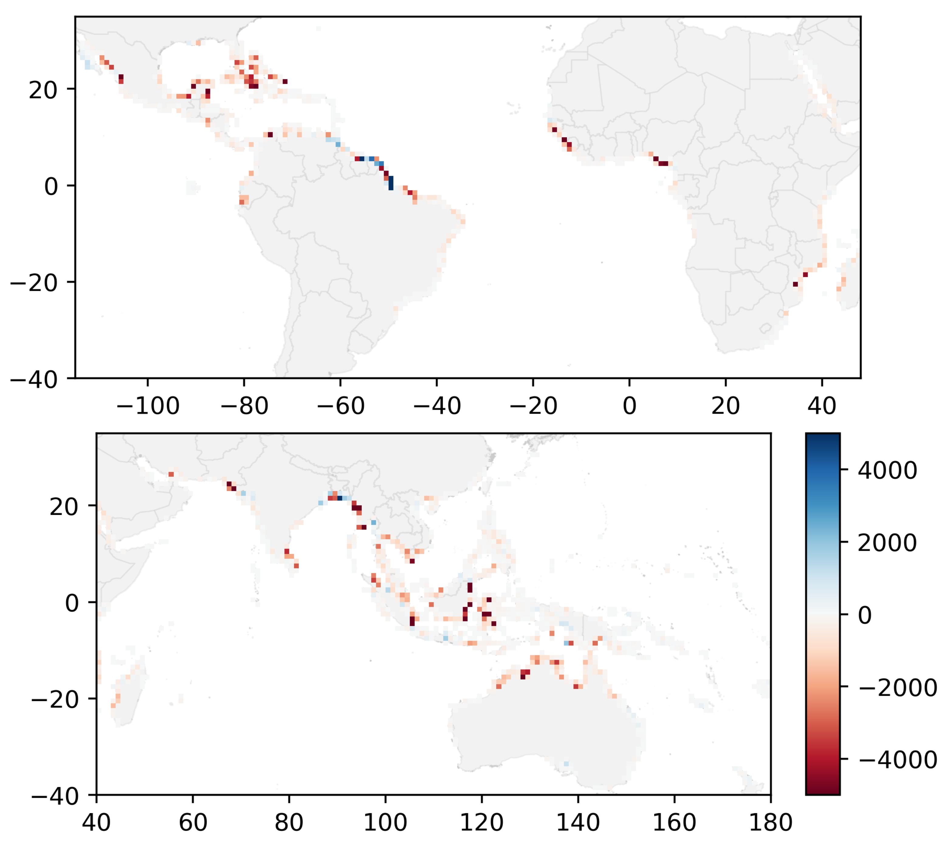
This study has provided global maps of mangrove extent for 11 annual epochs between 1996 and 2020, forming the latest version (v3.0) of the layers published by the Global Mangrove Watch. The changes from the GMW v2.5 2010 mangrove baseline [29] were mapped using the JAXA JERS-1 SAR, ALOS PALSAR and ALOS-2 PALSAR-2 L-band SAR data, identifying a net global mangrove loss of 3.4% which equates to −5245 km² with a 95th confidence interval of −13,587–1444 km² from 1996 to 2020. The large confidence intervals are mainly due to misregistration detected within the v1 release of the L-band SAR mosaics available at the time of this study. We would, therefore, not consider the independent gains and losses to be reliable, and we thus recommend only the net change estimates to be used. Mangroves are naturally dynamic as highlighted here by particular change hotspots, such as the Amazon River mouth, which has witnessed considerable gain in mangrove extent. Losses have occurred globally at a rate of about twice the gain, with more losses occurring at the start of the time series. This suggests that the rate of net global mangrove loss has slowed in recent years, but more work is required to better understand and confirm this trend with lower confidence intervals and considering the drivers of the changes. However, we would also advocate for an integrated near real-time monitoring system for the hotspots of loss that could support further conservation of these important coastal ecosystems.

References

1. Donato, D.C.; Kauffman, J.B.; Murdiyarso, D.; Kurnianto, S.; Stidham, M.; Kanninen, M. Mangroves among the most carbon-rich forests in the tropics. Nat. Geosci. 2011, 4, 293–297. [Google Scholar] [CrossRef]
2. Macreadie, P.I.; Costa, M.D.P.; Atwood, T.B.; Friess, D.A.; Kelleway, J.J.; Kennedy, H.; Lovelock, C.E.; Serrano, O.; Duarte, C.M. Blue carbon as a natural climate solution. Nat. Rev. Earth Environ. 2021, 2, 826–839. [Google Scholar] [CrossRef]
3. Li, S.; Chen, P.; Huang, J.; Hsueh, M.; Hsieh, L.; Lee, C.; Lin, H. Factors regulating carbon sinks in mangrove ecosystems. Glob. Chang. Biol. 2018, 24, 4195–4210. [Google Scholar] [CrossRef] [PubMed]
4. Su, J.; Friess, D.A.; Gasparatos, A. A meta-analysis of the ecological and economic outcomes of mangrove restoration. Nat. Commun. 2021, 12, 5050. [Google Scholar] [CrossRef] [PubMed]
5. Adame, M.F.; Connolly, R.M.; Turschwell, M.P.; Lovelock, C.E.; Fatoyinbo, T.; Lagomasino, D.; Goldberg, L.A.; Holdorf, J.; Friess, D.A.; Sasmito, S.D.; et al. Future carbon emissions from global mangrove forest loss. Glob. Chang. Biol. 2021, 27, 2856–2866. [Google Scholar] [CrossRef]
6. Richards, D.R.; Thompson, B.S.; Wijedasa, L. Quantifying net loss of global mangrove carbon stocks from 20 years of land cover change. Nat. Commun. 2020, 11, 4260. [Google Scholar] [CrossRef]
7. Sandilyan, S.; Kathiresan, K. Mangrove conservation: A global perspective. Biodivers. Conserv. 2012, 21, 3523–3542. [Google Scholar] [CrossRef]
8. Ermgassen, P.S.z.; Mukherjee, N.; Worthington, T.A.; Acosta, A.; Araujo, A.R.d.R.; Beitl, C.M.; Castellanos-Galindo, G.A.; Cunha-Lignon, M.; Dahdouh-Guebas, F.; Diele, K.; et al. Fishers who rely on mangroves: Modelling and mapping the global intensity of mangrove-associated fisheries. Estuar. Coast. Shelf Sci. 2021, 248, 107159. [Google Scholar] [CrossRef]
9. Spalding, M.; McIvor, A.; Tonneijck, F.; Tol, S.; van Eijk, P. Mangroves for Coastal Defence. Guidelines for Coastal Managers and Policy Makers; Technical Report; Wetlands International and The Nature Conservancy: Ede, The Netherlands, 2014; Available online: https://www.wetlands.org/publications/mangroves-for-coastal-defence/ (accessed on 1 July 2022).
10. Menéndez, P.; Losada, I.J.; Torres-Ortega, S.; Narayan, S.; Beck, M.W. The Global Flood Protection Benefits of Mangroves. Sci. Rep. 2020, 10, 4404. [Google Scholar] [CrossRef] [PubMed]
11. Buelow, C.A.; Connolly, R.M.; Turschwell, M.P.; Adame, M.F.; Ahmadia, G.N.; Andradi-Brown, D.A.; Bunting, P.; Canty, S.W.; Dunic, J.C.; Friess, D.A.; et al. Ambitious global targets for mangrove and seagrass recovery. Curr. Biol. 2022, 32, 1641–1649. [Google Scholar] [CrossRef] [PubMed]
12. Goldberg, L.; Lagomasino, D.; Thomas, N.; Fatoyinbo, T. Global declines in human-driven mangrove loss. Glob. Chang. Biol. 2020, 26, 5844–5855. [Google Scholar] [CrossRef] [PubMed]
13. Murray, N.J.; Worthington, T.A.; Bunting, P.; Duce, S.; Hagger, V.; Lovelock, C.E.; Lucas, R.; Saunders, M.I.; Sheaves, M.; Spalding, M.; et al. High-resolution mapping of losses and gains of Earth’s tidal wetlands. Science 2022, 376, 744–749. [Google Scholar] [CrossRef] [PubMed]
14. Duke, N.C.; Kovacs, J.M.; Griffiths, A.D.; Preece, L.; Hill, D.J.E.; Oosterzee, P.v.; Mackenzie, J.; Morning, H.S.; Burrows, D. Large-scale dieback of mangroves in Australia’s Gulf of Carpentaria: A severe ecosystem response, coincidental with an unusually extreme weather event. Mar. Freshw. Res. 2017, 678, 1816–1829. [Google Scholar] [CrossRef]
15. Gomes, L.E.d.O.; Sanders, C.J.; Nobrega, G.N.; Vescovi, L.C.; Queiroz, H.M.; Kauffman, J.B.; Ferreira, T.O.; Bernardino, A.F. Ecosystem carbon losses following a climate-induced mangrove mortality in Brazil. J. Environ. Manag. 2021, 297, 113381. [Google Scholar] [CrossRef]
16. Asbridge, E.; Lucas, R.; Rogers, K.; Accad, A. The extent of mangrove change and potential for recovery following severe Tropical Cyclone Yasi, Hinchinbrook Island, Queensland, Australia. Ecol. Evol. 2018, 8, 10416–10434. [Google Scholar] [CrossRef] [PubMed] [Green Version]
17. Awty-Carroll, K.; Bunting, P.; Hardy, A.; Bell, G. Using Continuous Change Detection and Classification of Landsat Data to Investigate Long-Term Mangrove Dynamics in the Sundarbans Region. Remote Sens. 2019, 11, 2833. [Google Scholar] [CrossRef] [Green Version]
18. Asbridge, E.; Lucas, R.; Ticehurst, C.; Bunting, P. Mangrove response to environmental change in Australia’s Gulf of Carpentaria. Ecol. Evol. 2016, 6, 3523–3539. [Google Scholar] [CrossRef] [PubMed] [Green Version]
19. Gatt, Y.M.; Andradi-Brown, D.A.; Ahmadia, G.N.; Martin, P.A.; Sutherland, W.J.; Spalding, M.D.; Donnison, A.; Worthington, T.A. Quantifying the Reporting, Coverage and Consistency of Key Indicators in Mangrove Restoration Projects. Front. For. Glob. Chang. 2022, 5, 720394. [Google Scholar] [CrossRef]
20. Sutherland, W.J.; Atkinson, P.W.; Butchart, S.H.; Capaja, M.; Dicks, L.V.; Fleishman, E.; Gaston, K.J.; Hails, R.S.; Hughes, A.C.; Anstey, B.L.; et al. A horizon scan of global biological conservation issues for 2022. Trends Ecol. Evol. 2021, 37, 95–104. [Google Scholar] [CrossRef] [PubMed]
21. Murray, N.J.; Kennedy, E.V.; Álvarez Romero, J.G.; Lyons, M.B. Data Freshness in Ecology and Conservation. Trends Ecol. Evol. 2021, 36, 485–487. [Google Scholar] [CrossRef] [PubMed]
22. Hamilton, S.E.; Casey, D. Creation of a high spatio-temporal resolution global database of continuous mangrove forest cover for the 21st century (CGMFC-21). Glob. Ecol. Biogeogr. 2016, 25, 729–738. [Google Scholar] [CrossRef]
23. Giri, C.; Ochieng, E.; Tieszen, L.L.; Zhu, Z.; Singh, A.; Loveland, T.; Masek, J.; Duke, N. Status and distribution of mangrove forests of the world using earth observation satellite data. Glob. Ecol. Biogeogr. 2011, 20, 154–159. [Google Scholar] [CrossRef]
24. Hansen, M.C.; Potapov, P.V.; Moore, R.; Hancher, M.; Turubanova, S.A.; Tyukavina, A.; Thau, D.; Stehman, S.V.; Goetz, S.J.; Loveland, T.R.; et al. High-Resolution Global Maps of 21st-Century Forest Cover Change. Science 2013, 342, 850–853. [Google Scholar] [CrossRef] [PubMed] [Green Version]
25. Bunting, P.; Rosenqvist, A.; Lucas, R.; Rebelo, L.M.; Hilarides, L.; Thomas, N.; Hardy, A.; Itoh, T.; Shimada, M.; Finlayson, M. Global Mangrove Watch (1996–2016) Version 2.0. Zenodo 2019. [Google Scholar] [CrossRef]
26. Global Mangrove Watch Portal. Available online: https://globalmangrovewatch.org (accessed on 9 June 2022).
27. Bunting, P.; Rosenqvist, A.; Lucas, R.; Rebelo, L.M.; Hilarides, L.; Thomas, N.; Hardy, A.; Itoh, T.; Shimada, M.; Finlayson, C. The Global Mangrove Watch—A New 2010 Global Baseline of Mangrove Extent. Remote Sens. 2018, 10, 1669. [Google Scholar] [CrossRef] [Green Version]
28. JAXA Kyoto & Carbon Initiative. Available online: www.eorc.jaxa.jp/ALOS/en/activity/kyoto/mangrovewatch_e.htm (accessed on 7 July 2022).
29. Bunting, P.; Rosenqvist, A.; Hilarides, L.; Lucas, R.; Thomas, N. Global Mangrove Watch: Updated 2010 Mangrove Forest Extent (v2.5). Remote Sens. 2022, 14, 1034. [Google Scholar] [CrossRef]
30. UNEP SDG 6.6.1 App. Available online: www.sdg661.app (accessed on 7 July 2022).
31. Bunting, P.; Clewley, D.; Lucas, R.M.; Gillingham, S. The Remote Sensing and GIS Software Library (RSGISLib). Comput. Geosci. 2014, 62, 216–226. [Google Scholar] [CrossRef]
32. Bunting, P.; Gillingham, S. The KEA image file format. Comput. Geosci. 2013, 57, 54–58. [Google Scholar] [CrossRef]
33. PBProcessTools. Available online: https://www.remotesensing.info/pbprocesstools/ (accessed on 10 December 2021).
34. Shimada, M.; Itoh, T.; Motohka, T.; Watanabe, M.; Shiraishi, T.; Thapa, R.; Lucas, R. New global forest/non-forest maps from ALOS PALSAR data (2007–2010). Remote Sens. Environ. 2014, 155, 13–31. [Google Scholar] [CrossRef]
35. Thomas, N.; Lucas, R.; Itoh, T.; Simard, M.; Fatoyinbo, L.; Bunting, P.; Rosenqvist, A. An approach to monitoring mangrove extents through time-series comparison of JERS-1 SAR and ALOS PALSAR data. Wetl. Ecol. Manag. 2014, 23, 1–15. [Google Scholar] [CrossRef]
36. Thomas, N.; Lucas, R.; Bunting, P.; Hardy, A.; Rosenqvist, A.; Simard, M. Distribution and drivers of global mangrove forest change, 1996–2010. PLoS ONE 2017, 12, e0179302. [Google Scholar] [CrossRef] [PubMed] [Green Version]
37. Thomas, N.; Bunting, P.; Lucas, R.; Hardy, A.; Rosenqvist, A.; Fatoyinbo, T. Mapping Mangrove Extent and Change: A Globally Applicable Approach. Remote Sens. 2018, 10, 1466. [Google Scholar] [CrossRef] [Green Version]
38. Bunting, P.; Labrosse, F.; Lucas, R. A multi-resolution area-based technique for automatic multi-modal image registration. Image Vis. Comput. 2010, 28, 1203–1219. [Google Scholar] [CrossRef]
39. GEBCO Compilation Group. GEBCO 2020 Grid. Online, 2020. Available online: https://doi.org/10.5285/a29c5465-b138-234d-e053-6c86abc040b9 (accessed on 1 July 2022).
40. Pekel, J.; Cottam, A.; Gorelick, N.; Belward, A.S. High-resolution mapping of global surface water and its long-term changes. Nature 2016, 540, 1–19. [Google Scholar] [CrossRef] [PubMed]
41. Zhao, Y.; Nasrullah, Z.; Li, Z. PyOD: A Python Toolbox for Scalable Outlier Detection. J. Mach. Learn. Res. 2019, 20, 1–7. [Google Scholar]
42. Simard, M.; Fatoyinbo, L.; Smetanka, C.; Rivera-Monroy, V.H.; Castañeda-Moya, E.; Thomas, N.; Stocken, T.V.D. Mangrove canopy height globally related to precipitation, temperature and cyclone frequency. Nat. Geosci. 2019, 12, 40–45. [Google Scholar] [CrossRef]
43. Murray, N.J.; Phinn, S.R.; DeWitt, M.; Ferrari, R.; Johnston, R.; Lyons, M.B.; Clinton, N.; Thau, D.; Fuller, R.A. The global distribution and trajectory of tidal flats. Nature 2018, 565, 1–22. [Google Scholar] [CrossRef] [PubMed]
44. Olofsson, P.; Foody, G.M.; Stehman, S.V.; Woodcock, C.E. Making better use of accuracy data in land change studies: Estimating accuracy and area and quantifying uncertainty using stratified estimation. Remote Sens. Environ. 2013, 129, 122–131. [Google Scholar] [CrossRef]
45. Rosenqvist, A.; Forsberg, B.R.; Pimentel, T.; Rauste, Y.A.; Richey, J.E. The use of spaceborne radar data to model inundation patterns and trace gas emissions in the central Amazon floodplain. Int. J. Remote Sens. 2002, 23, 1303–1328. [Google Scholar] [CrossRef]
46. Standard Country or Area Codes for Statistical Use. Available online: https://unstats.un.org/unsd/methodology/m49 (accessed on 10 June 2022).
47. Lymburner, L.; Bunting, P.; Lucas, R.; Scarth, P.; Alam, I.; Phillips, C.; Ticehurst, C.; Held, A. Mapping the multi-decadal mangrove dynamics of the Australian coastline. Remote. Sens. Environ. 2019, 238, 111185. [Google Scholar] [CrossRef]
48. Wilkie, M.L.; Fortuna, S. Forest Resources Assessment (FRA) 2005 Thematic Study on Mangroves; Technical Report; Forest Resources Division, Food and Agriculture Organization of the United Nations: Rome, Italy, 2007. [Google Scholar]
49. Don T De Alban, J.; Jamaludin, J.; Wen, D.W.D.; Than, M.M.; Webb, E.L. Improved estimates of mangrove cover and change reveal catastrophic deforestation in Myanmar. Environ. Res. Lett. 2020, 15, 034034. [Google Scholar] [CrossRef]
50. Zhang, M.; Liu, N.; Harper, R.; Li, Q.; Liu, K.; Wei, X.; Ning, D.; Hou, Y.; Liu, S. A global review on hydrological responses to forest change across multiple spatial scales: Importance of scale, climate, forest type and hydrological regime. J. Hydrol. 2017, 546, 44–59. [Google Scholar] [CrossRef] [Green Version]
51. Zhao, B.; Lei, H.; Yang, D.; Yang, S.; Santisirisomboon, J. Runoff and sediment response to deforestation in a large Southeast Asian monsoon watershed. J. Hydrol. 2022, 606, 127432. [Google Scholar] [CrossRef]
52. Li, T.; Wang, S.; Liu, Y.; Fu, B.; Gao, D. Reversal of the sediment load increase in the Amazon basin influenced by divergent trends of sediment transport from the Solimões and Madeira Rivers. Catena 2020, 195, 104804. [Google Scholar] [CrossRef]
53. Giri, C.; Long, J. Is the Geographic Range of Mangrove Forests in the Conterminous United States Really Expanding? Sensors 2016, 16, 2010. [Google Scholar] [CrossRef] [Green Version]
54. Cavanaugh, K.C.; Dangremond, E.M.; Doughty, C.L.; Williams, A.P.; Parker, J.D.; Hayes, M.A.; Rodriguez, W.; Feller, I.C. Climate-driven regime shifts in a mangrove-salt marsh ecotone over the past 250 years. Proc. Natl. Acad. Sci. USA 2019, 116, 21602–21608. [Google Scholar] [CrossRef] [Green Version]
55. Lagomasino, D.; Fatoyinbo, T.; Castañeda-Moya, E.; Cook, B.D.; Montesano, P.M.; Neigh, C.S.R.; Corp, L.A.; Ott, L.E.; Chavez, S.; Morton, D.C. Storm surge and ponding explain mangrove dieback in southwest Florida following Hurricane Irma. Nat. Commun. 2021, 12, 4003. [Google Scholar] [CrossRef]
56. Agbagwa, I.O.; Ndukwu, B.C. Oil and Gas Pipeline Construction-Induced Forest Fragmentation and Biodiversity Loss in the Niger Delta, Nigeria. Nat. Resour. 2014, 05, 698. [Google Scholar] [CrossRef] [Green Version]
57. Lucas, R.; Kerchove, R.V.D.; Otero, V.; Lagomasino, D.; Fatoyinbo, L.; Omar, H.; Satyanarayana, B.; Dahdouh-Guebas, F. Structural characterisation of mangrove forests achieved through combining multiple sources of remote sensing data. Remote Sens. Environ. 2020, 237, 111543. [Google Scholar] [CrossRef]
58. Lucas, R.; Otero, V.; Kerchove, R.V.D.; Lagomasino, D.; Satyanarayana, B.; Fatoyinbo, T.; Dahdouh-Guebas, F. Monitoring Matang’s Mangroves in Peninsular Malaysia through Earth observations: A globally relevant approach. Land Degrad. Dev. 2021, 32, 354–373. [Google Scholar] [CrossRef]
59. Worthington, T.A.; Andradi-Brown, D.A.; Bhargava, R.; Buelow, C.; Bunting, P.; Duncan, C.; Fatoyinbo, L.; Friess, D.A.; Goldberg, L.; Hilarides, L.; et al. Harnessing Big Data to Support the Conservation and Rehabilitation of Mangrove Forests Globally. ONE Earth 2020, 3, 260. [Google Scholar] [CrossRef]
60. UN Biodiversity Lab. Available online: map.unbiodiversitylab.org (accessed on 7 July 2022).
61. WCMC Ocean Data Viewer. Available online: data.unep-wcmc.org/datasets/45 (accessed on 7 July 2022).
62. WCMC Ocean+ Habitats. Available online: habitats.oceanplus.org (accessed on 7 July 2022).
63. WRI Global Forest Watch. Available online: www.globalforestwatch.org (accessed on 7 July 2022).
64. WRI Resource Watch. Available online: www.wri.org/initiatives/resource-watch (accessed on 7 July 2022).
65. JAXA Earth Observation Research Center Data Platform. Available online: www.eorc.jaxa.jp/ALOS/en/dataset/fnfe.htm (accessed on 7 July 2022).
66. Global 25m Resolution PALSAR-2 Mosaic (Ver. 2.1.0) Dataset Description. Available online: https://www.eorc.jaxa.jp/ALOS/en/dataset/pdf/DatasetDescription_PALSAR2_Mosaic_ver210.pdf (accessed on 3 July 2022).
67. Wilkie, M.L.; Fortuna, S. Status and Trends in Mangrove Area Extent Worldwide; Technical Report; The Food and Agriculture Organization (FAO): Rome, Italy, 2003; Available online: http://www.fao.org/3/j1533e/J1533E02.htm (accessed on 1 July 2022).
68. Nwobi, C.; Williams, M.; Mitchard, E.T.A. Rapid Mangrove Forest Loss and Nipa Palm (Nypa fruticans) Expansion in the Niger Delta, 2007–2017. Remote Sens. 2020, 12, 2344. [Google Scholar] [CrossRef]
69. Global Mangrove Alliance. Available online: www.mangrovealliance.org (accessed on 10 June 2022).
70. Spalding, M.D.; Leal, M. The State of the World’s Mangroves 2021. Technical Report. Global Mangrove Alliance. 2021. Available online: https://www.mangrovealliance.org/mangrove-forests (accessed on 1 July 2022).
Figure 1. Methodology Workflow.
Remotesensing 14 03657 g001
Figure 2. Examples of mangrove change identified within a time-series composite of L-Band HH SAR data from 1996, 2010 and 2020 in RGB. Areas in red and yellow highlight loss of mangroves (high L-HH in 1996 but low in later years = red; L-HH is high in 1996 and 2007 but low in 2010 = yellow) while gains are represented by shades of blue (i.e., low L-band HH backscatter in 1996 but increased in both 2010 and 2020 (cyan) and in 2020 only (blue)). Examples of change are mangrove loss and/or gain in (a) the Sundarbans, (b) French Guiana, (c) Sulawesi (Indonesia) and (d) Sumatra (Indonesia). Observed losses are primarily through coastal erosion (a,b) and deforestation (e.g., for aquaculture development (c) whilst gains are primarily through colonisation of coastal sediment banks (b,d).
Remotesensing 14 03657 g002
Figure 3. Examples of the contextual regions defining the non-mangrove regions for change (a) from Venezuela, where mangroves are expanding, (b) from Sumatra, Indonesia, in a region of aquaculture and (c) from The Bahamas, where the coastline is complex with many small islands. The green areas are the 2010 v2.5 mangrove baseline, while the blue areas are the contextual areas, indicating there is the potential of mangrove occurrence.
Remotesensing 14 03657 g003
Figure 4. Example histograms with the thresholds for defining (a) mangrove and (b) non-mangrove thresholds.
Remotesensing 14 03657 g004
Figure 5. Illustrating the histograms of 2010 HV ALOS PALSAR backscatter from the 2010 mangrove baseline and non-mangrove contextual regions for project GMW-09-003, Sumatra, Indonesia. These histograms are representative of the other projects and both HH and HV polarisations. (a) The mangrove HV histogram and (b) Q-Q plot illustrating that the majority of the histogram is normal will a short tail in the lower values. (c) The non-mangrove HV histogram and (d) Q-Q plot illustrating that the majority of the histogram is normal with a small tail in the higher values.
Remotesensing 14 03657 g005
Figure 6. An updated version of GMW geographic projects from [27] used to define the change thresholds. The projects are defined in two levels, the first as broad geography areas (e.g., South America) and then within those regions, the second level of projects are defined. Examples are shown for South America and South East Asia. Colours were randomly assigned to illustrate the different projects at the two levels, where the 1 × 1 tiles have the same colour they are within the same project at that level.
Remotesensing 14 03657 g006
Figure 7. Sensitivity of the mangrove (a) and non-mangrove (b) change thresholds. These plots illustrate the percentage of change in the number of mangrove or non-mangrove pixels classified with the change in threshold, where the red line indicates the threshold used.
Remotesensing 14 03657 g007
Figure 8. Site locations for assessing the accuracy of the mangrove changes.
Remotesensing 14 03657 g008
Figure 9. Examples of the mangrove change results. (a) Mangrove loss in Sulawesi, Indonesia, (b) Mangrove gain in Amazon Delta, (c,d) natural mangrove dynamics in Guyana, (e,f) anthropogenic mangrove dynamics in Guinea-Bissau and (g) an example of false mangrove gain and loss due to misregistration.
Remotesensing 14 03657 g009
Figure 10. Net change in mangrove extent (in ha) illustrating the locations of mangrove change hotspots on a 1 × 1 degree grid. Areas of red show a net loss while areas in blue a net gain.
Remotesensing 14 03657 g010
Figure 11. Accuracy of the individual classes using the F1-score with an increasing number of accuracy samples.
Remotesensing 14 03657 g011
Figure 12. Visual comparison of this study compared to the L-band SAR data and the GMW v2.0 [25], Murray et al. [13] and Goldberg et al. [12] datasets. Mangroves for an area of loss due to aquaculture in East Kalimantan, Indonesia (ae) and a dynamic river estuary in Papua New Guinea (fj) are shown. The Red and Yellow regions in the SAR images (a,f) correspond with loss, Blue with gain and White and Black as no change. Within the mangrove maps (be,gj) Blue represents detected mangrove gains and Red represents detected losses.
Remotesensing 14 03657 g012