Retrieval and Uncertainty Analysis of Land Surface Reflectance Using a Geostationary Ocean Color Imager

Abstract

Land surface reflectance (LSR) is well known as an essential variable to understand land surface properties. The Geostationary Ocean Color Imager (GOCI) be able to observe not only the ocean but also the land with the high temporal and spatial resolution thanks to its channel specification. In this study, we describe the land atmospheric correction algorithm and present the quality of results through comparison with Moderate Resolution Imaging Spectroradiometer (MODIS) and in-situ data for GOCI-II. The GOCI LSR shows similar spatial distribution and quantity with MODIS LSR for both healthy and unhealthy vegetation cover. Our results agreed well with in-situ-based reference LSR with a high correlation coefficient (>0.9) and low root mean square error (<0.02) in all 8 GOCI channels. In addition, seasonal variation according to the solar zenith angle and phenological dynamics in time-series was well presented in both reference and GOCI LSR. As the results of uncertainty analysis, the estimated uncertainty in GOCI LSR shows a reasonable range (<0.04) even under a high solar zenith angle over 70°. The proposed method in this study can be applied to GOCI-II and can provide continuous satellite-based LSR products having a high temporal and spatial resolution for analyzing land surface properties.

1. Introduction

Land surface reflectance (LSR) is defined as the ratio of upwelling solar radiation reflected by a land surface to downwelling solar radiation for specific solar and viewing geometries [1] and it is determined by the intrinsic property of the land surface as well as observation geometry [2]. Because LSR is sensitive to changes in land surface caused by both natural and artificial factors such as vegetation growth, snowfall, desertification, and urbanization [2,3,4,5], it is widely utilized in studies on land environmental changes. Painter et al. [6] developed a radiative forcing model to retrieve the amount of land surface radiation caused from light absorption by dirty snow using Moderate Resolution Imaging Spectroradiometer (MODIS) LSR products. Potapov et al. [7] presented a consistent long-term LSR database based on Landsat satellite data for detecting changes in land cover both globally and locally. Thus, accurate LSR data are necessary to understand changes in the land surface and to analyze land surface properties.

Atmospheric correction to remove atmospheric effects from satellite observations is essential for terrestrial surface analysis [8,9,10]. It is divided into relative and absolute atmospheric corrections [11,12,13]. Relative atmospheric correction methods such as the empirical line method and improved dark-object subtraction are a statical-based method [14], whereas absolute atmospheric correction methods are physical-based methods dependent on the radiative transfer model (RTM). For LSR retrieval, absolute atmospheric correction outperforms the empirical method, because it considers local geographic and atmospheric conditions during RTM simulation [15,16,17]. Thus, RTMs such as MODerate resolution atmospheric TRANsmission (MODTRAN) and Second Simulation of a Satellite Signal in the Solar Spectrum (6S) have been used with various software programs for atmospheric correction [18,19,20,21,22,23,24,25,26]. In addition, RTM has been used in LSR retrieval algorithms of MODIS [27], the Visible Infrared Imaging Radiometer Suite [28], and Advanced Baseline Imager [29] for operational purposes.

To remove atmospheric effects through absolute atmospheric correction, a-priori information such as atmospheric conditions (water vapor and ozone amount, aerosol information) and geometric conditions (solar zenith angle [SZA], viewing zenith angle [VZA], and relative azimuth angle [RAA]) are required. Satellite data products with sufficient temporal and spatial resolutions have been generally used as a-priori information in atmospheric correction of satellite observations [27]; however, climate data, the European Centre for Medium-Range Weather Forecasts (ECMWF) reanalysis data or the National Centers for Environmental Prediction reanalysis data have also been used [30,31,32]. However, since such a priori information is not truth, it contains inherent uncertainty, which directly affects the quality of the calculated LSR. Especially, error in aerosol optical depth (AOD) is one of the most influential sources of uncertainty in LSR retrieval [33,34,35]. This uncertainty can cause significant errors in subsequent applications and alter the inferred conclusion [36]. Despite the importance of uncertainty analysis of remotely sensed products, input data-induced uncertainties in remotely sensed LSR data are rarely quantitatively analyzed [37,38]. Most operational satellite-based products provide users with the associated quality flags; however, the obtained information cannot fully explain the data uncertainties [39]. Therefore, to guarantee the quality of the satellite-based variables, the uncertainties associated with the sensed variables need to be measured and provided to users.

The Geostationary Ocean Color Imager (GOCI), which is the world’s first geostationary ocean color sensor, hourly transmits images during the daytime. GOCI totals eight images per day, by observing a local area of 2500 × 2500 km (center latitude and longitude are 36°N and 130°E, respectively). GOCI has eight spectral bands, from visible (VIS) light to near-infrared (NIR), and it monitors the marine environment around the Korean Peninsula [40,41]. These spectral bands allow monitoring of the atmosphere and land surface because the short blue and NIR bands can reveal aerosols and vegetation, respectively [42,43]. Thus, GOCI, like other ocean color sensors, is widely used in terrestrial remote sensing applications. Kim et al. [44] estimated normalized difference vegetation index (NDVI) data over different composite periods (4, 8, 12, and 16 days) using GOCI imagery based on an optimized bidirectional reflectance distribution function (BRDF). Ke et al. [45] estimated NDVI from GOCI LSR and used it to analyze the characteristics of Landsat-8/OLI-derived NDVI. Son and Kim [46] conducted a feasibility study to produce a land cover map using principal component analysis, K-means clustering, and GOCI NDVI via BRDF modeling. Yeom et al. [47] and Kim et al. [48] have suggested novel cloud masking methods using BRDF-based background surface reflectance and Top-Of-Atmosphere (TOA) reflectance of GOCI. The abovementioned studies estimated LSR using absolute atmospheric correction. As input data, they used a daily product that does not consider the diurnal variability of the atmosphere; however, uncertainty analysis was not performed.

GOCI-II, with 26 operational products, has been developed as the next-generation instrument of GOCI. To meet the increasing land applications of GOCI, GOCI-II contains four land variables (LSR, vegetation index, land surface albedo, and land cover) [49]. All of the GOCI-II land products directly or indirectly use LSR as input data [50]; thus, their accuracy and stability depend on those of LSR. Therefore, in addition to LSR retrieval and validation, uncertainty analysis of the data is essential to ensure quality of subsequent land products.

In this study, we aimed to (1) develop an operational atmospheric correction algorithm for GOCI-II using RTM simulations and (2) analyze the accuracy and input data-induced uncertainty in estimated LSR by comparing the LSR data with in situ reference data. Owing to the short operation period of GOCI-II (since October 2020), the corresponding reference data are limited, whereas a large amount of GOCI reference data can be obtained from the observations of the 2016 Korea–United States (KORUS) campaign; therefore, we used GOCI measurements as proxy data instead of GOCI-II. In addition, the channel specifications and observation systems of GOCI are similar to those of GOCI-II.

The remaining parts of this paper are organized as follows: Section 2 describes the materials used in this study. Section 3 explains the methods for retrieval, validation, and uncertainty analysis of LSR. Section 4 presents the result of qualitative comparison with other satellite-based LSR, and the accuracy and uncertainty analysis results of estimated LSR. Lastly, Section 5 summarizes our findings.

2. Materials

2.1. Satellite Data

The GOCI mounted on the Communication, Ocean and Meteorological Satellite was designed with a target area of 2500 km × 2500 km, to monitor the color of the ocean surrounding the Korean Peninsula, Northeast Asia (Figure 1). GOCI has eight spectral channels, whose specifications are presented in

Table 1. GOCI channel specifications (Ryu et al. [40]).

Band	Central WaveLength (nm)	Band Width (nm)	Primary Use
Band 1	412	20	Yellow substance and turbidity
Band 2	443	20	Chlorophyll absorption maximum
Band 3	490	20	Chlorophyll and other pigments
Band 4	555	20	Turbidity, suspended sediment
Band 5	660	20	Baseline of fluorescence signal, chlorophyll, suspended sediment
Band 6	680	10	Atmospheric correction and fluorescence signal
Band 7	745	20	Atmospheric correction and baseline of fluorescence signal
Band 8	865	40	Aerosol optical thickness, vegetation, water vapor reference over the ocean

. GOCI provides hourly observations from 00 UTC to 07 UTC, with a spatial resolution of 500 m, which exceeds those of other geostationary satellites observing Northeast Asia, such as the Advanced Meteorological Imager (AMI) and Advanced Himawari Imager [40]. Owing to its advantage of high spatial and temporal resolutions, GOCI has been widely used for land surface, atmosphere, and ocean monitoring [47,48]. In this study, we used GOCI Level 1B (L1B) and GOCI AOD products for atmospheric correction. These datasets were provided by the Korea Ocean Satellite Center (KOSC) in the Korea Institute of Ocean Science and Technology (KIOST). GOCI L1B data were saved as a digital number (DN). We converted the data to top-of-atmosphere (TOA) radiance using calibration coefficients (Equation (1)):

$$L_i=D{N}_i\times a_i+b_i$$

(1)

where 𝐿_𝑖 is the TOA radiance (W⋅m⁻²⋅sr⁻¹⋅μm⁻¹) of GOCI image in band 𝑖; 𝐷𝑁_𝑖 is the digital number from the GOCI image in band 𝑖; 𝑎_𝑖 and 𝑏_𝑖 are calibration coefficients for gain and offset, respectively.

The GOCI AOD product was generated using the Yonsei aerosol retrieval (YEAR) version 2 algorithm, which features updated cloud masking and LSR calculation methods [51]. Cloud masking was performed in 13 steps using GOCI TOA reflectance. The details of the threshold for cloud masking can be found in Choi et al. [51]. Through these improvements in the YAER version2 algorithm, GOCI AOD shows good agreements with Aerosol Robotic Network (AERONET) measurements. Especially, for the land domain, GOCI AOD products have a lower uncertainty (±(0.079 + 0.137 × AOD) [44]) than the Advanced Himawari Imager AOD product (±(0.1 + 0.3 × AOD) [52]). Therefore, GOCI AOD is suitable for atmospheric correction and was used not only as input data for atmospheric correction, but also for masking clouds and snow cover.

For qualitative comparison, we also used the MODIS LSR (MOD09) swath product, which satisfies the validation stage 2 criteria of the Committee on Earth Observation Satellites’ Land Product Validation subgroup. The atmospheric correction accuracy of MODIS LSR is ±(0.005 + 0.05 × LSR) under favorable conditions (non-high aerosol amount) [53]. The spectral ranges of MODIS red and NIR bands are similar to those of the corresponding GOCI bands and are widely used in land surface environmental analyses; therefore, we used only MODIS LSR of bands 1 (red) and 2 (NIR). These bands have a spatial resolution of 250 m; however, we used data aggregated into 500 m resolution to match the resolution with the GOCI spatial resolution.

2.2. Copernicus Atmosphere Monitoring Service Near-Real-Time Data

Since January 2015, after the Monitoring Atmospheric Composition and Climate project (2009–2014), atmospheric composition and climate have been monitored by the ECMWF-operated Copernicus Atmosphere Monitoring Service (CAMS) [54]. The CAMS combines numerical models and observations from remote sensing satellites and other sources such as ground-based observation stations, aircraft, ships, and sondes. Based on the observations, it provides continuous data and value-added information on atmospheric composition and its variabilities at global and regional scales. The CAMS assimilation system uses incremental four-dimensional variational data assimilation. It is based on the ECMWF integrated forecasting system and was developed during three Monitoring Atmospheric Composition and Climate research projects [55]. The CAMS offers three types (analysis, forecast, and reanalysis) of information about trace gases, greenhouse gases, and aerosols. The CAMS near-real-time dataset includes daily analyses and forecasts of geophysical variables of air quality and atmospheric composition, ozone layer and ultraviolet radiation, emissions and surface fluxes, solar radiation, and climate forcing. These products are validated by CAMS-84, which is a CAMS subproject for validating service products every three months at global and regional scales [56]. In this study, CAMS-provided total precipitable water (TPW), and total column ozone (TCO) data were used in the atmospheric correction process to consider atmospheric conditions at observation times. Although these data have lower temporal and spatial resolutions (daily and 0.125°, respectively) than GOCI data, they are suitable because they do not have high sensitivity in LSR estimation, and GOCI TPW and TCO are unavailable [33]. CAMS TPW and TCO used in this study were interpolated from 0.125 degrees to 0.25 km to match spatial resolution with GOCI by a cubic-spline interpolation. Since only one CAMS data can be acquired per day, it is not interpolated according to time. CAMS TPW and TCO of specific dates were used for atmospheric correction of all 8 GOCI observations (from 00 to 07 UTC) acquired on the same date.

2.3. AERONET Data

The AERONET project is a federation of ground-based remote sensing aerosol networks greatly expanded by collaborators from universities, national agencies, and institutes. The project provides aerosol properties, inversion products, and precipitable water for wavelengths of 340–1640 nm [57]. For several decades, AERONET has provided numerous observations that cover large spatial and temporal ranges, and its data have been used for various purposes, including satellite product validation. We used a level-2 AOD product that contained TPW, TCO, and AOD to generate in situ reference LSR datasets and calculated uncertainties in atmospheric parameters. Level 2 is the highest quality level among Version 3 AOD data and means “quality assured”. The quality assurance criteria can be found in Holben et al. [57]. We obtained AERONET measurements for 28 sites from the AERONET website (https://aeronet.gsfc.nasa.gov/ (accessed on 13 September 2021)). Additional information of AERONET sites used in this study is presented in

Table 2. List of AERONET sites used in this study.

Sites	Latitude (°)	Longitude (°)	Altitude (m)	Number of Matchups
Anmyon	36.53854	126.3302	47	326
Baengnyeong	37.96611	124.6303	136	266
Chiba_University	35.6247	140.1038	60	228
DRAGON_GangneungWNU	37.771	128.867	60	2
DRAGON_Hankuk_UFS	37.33883	127.2658	167	21
EPA-NCU	24.96753	121.1855	144	9
Fukuoka	33.524	130.475	30	103
Gangneung_WNU	37.771	128.867	60	452
Gosan_SNU	33.29222	126.1617	72	67
Gwangju_GIST	35.22828	126.8431	52	132
Hankuk_UFS	37.33883	127.2658	167	201
Hokkaido_University	43.0755	141.3407	59	162
KORUS_Baeksa	37.41156	127.5691	64	144
KORUS_Daegwallyeong	37.68712	128.7587	837	37
KORUS_Iksan	35.9622	127.0052	84	173
KORUS_Kyungpook_NU	35.88999	128.6064	65	151
KORUS_Olympic_Park	37.52165	127.1242	45	122
KORUS_Songchon	37.33849	127.4895	90	115
KORUS_Taehwa	37.31248	127.3103	152	90
KORUS_UNIST_Ulsan	35.5819	129.1897	106	133
Niigata	37.846	138.942	10	243
Noto	37.33444	137.1369	200	130
Osaka	34.65093	135.5906	50	204
Pusan_NU	35.23535	129.0825	78	333
Seoul_SNU	37.45806	126.9511	116	312
Taipei_CWB	25.01468	121.5384	26	6
Ussuriysk	43.7004	132.1635	280	368
Yonsei_University	37.56443	126.9348	97	325

. The differences between two measurements temporally and spatially can introduce errors on validation and uncertainty analysis [58]; therefore, in this study, only data satisfying all of the following criteria were used for further analysis: (1) the difference in observation time between AERONET and GOCI must be less than 10 minutes, (2) The location of the AERONET site must be within half a pixel of the GOCI. The large amounts of data were discarded due to spatiotemporal criteria, and we used 4855 matchups for validation and uncertainty analysis.

3. Methods

The following three processing steps were used in this study: (1) LSR retrieval, (2) validation, and (3) uncertainty analysis. The adopted method, assumptions, and background for each step are described in the following subsections.

3.1. LSR Retrieval

For LSR estimation from GOCI, we used the 6S vector (6SV) radiative transfer code, which is an improved version of the Simulation of a Satellite Signal in the Solar Spectrum [59]. This code is based on successive orders of scattering approximations and can describe the polarization effect using four Stokes vector components [60]. 6SV is one of the widely used radiative transfer codes for atmospheric correction of satellite images because of its high accuracy. According to Kotchenova et al. [61], 6SV showed an error lower than 1% when compared with the Monte Carlo code and Coulson’s tabulated value, which are well-known benchmarks. This error is lower than the results of other RTMs (spherical harmonics [SHARM], MODTRAN, and radiative transfer [RT3]) [61]. In the 6SV, the LSR can be calculated from TOA radiance measured by satellite through Equation (2).

$${\rho }_s\left({\theta }_s,{\theta }_v,\varphi \right) =\frac{\frac{L\left({\theta }_s,{\theta }_v,\varphi \right)}{T_g\left({\theta }_s,{\theta }_v\right)T^{\downarrow }\left({\theta }_s\right)T^{\uparrow }\left({\theta }_s\right)}-\frac{{\rho }_{R+A}}{T^{\downarrow }\left({\theta }_s\right)T^{\uparrow }\left({\theta }_s\right)}}{1+S\left(\frac{L\left({\theta }_s,{\theta }_v,\varphi \right)}{T_g\left({\theta }_s,{\theta }_v\right)T^{\downarrow }\left({\theta }_s\right)T^{\uparrow }\left({\theta }_s\right)}-\frac{{\rho }_{R+A}}{T^{\downarrow }\left({\theta }_s\right)T^{\uparrow }\left({\theta }_s\right)}\right)}$$

(2)

where, ${\rho }_s$ means the LSR; $L$ is the TOA radiance; ${\theta }_s$, ${\theta }_v$ and $\varphi$ indicates the SZA, VZA, and RAA, respectively; $T_g$ is total transmittance of atmospheric gases such as water vapor and ozone; $T^{\downarrow }$ and $T^{\uparrow }$ are total transmittances of the atmosphere for upward and downward radiance paths, respectively; ${\rho }_{R+A}$ is total scattering of molecules and aerosols; $S$ is spherical albedo. The 6SV provides three coefficients called xa, xb, and xc to simplify Equation (2). Using these coefficients, Equation (2) can be presented as following equations:

$${\rho }_s\left({\theta }_s,{\theta }_v,\varphi \right)=\frac{xa·L\left({\theta }_s,{\theta }_v,\varphi \right)-xb}{1+xc\left(xa·L\left({\theta }_s,{\theta }_v,\varphi \right)-xb\right)}$$

(3)

with

$$xa=\frac{1}{T_g\left({\theta }_s,{\theta }_v\right)T^{\downarrow }\left({\theta }_s\right)T^{\uparrow }\left({\theta }_s\right)}$$

(4)

$$xb=\frac{{\rho }_{R+A}}{T^{\downarrow }\left({\theta }_s\right)T^{\uparrow }\left({\theta }_s\right)}$$

(5)

$$xc=S$$

(6)

In the above equations, $xa$ is inverse of the transmittance; $xb$ is atmospheric reflectance; $xc$ reflects the spherical albedo. However, atmospheric effect simulation using the 6SV code is time-consuming because of complex computation; thus, it is difficult to use 6SV directly for operational atmospheric correction of a satellite image. Therefore, in this study, we used the lookup table (LUT) approach, which is widely used in 6SV-based atmospheric correction for operation and research purposes [28,62,63]. The LUT approach involves a simple index-based calculation instead of the complex calculation of 6SV, and avoids repetitive calculations; thus, it can significantly reduce processing time. However, although the LUT approach is suitable for the operational algorithm, the interval of LUT entries can cause errors in the retrieved LSR; especially, the relative error can rise to 60% at 470 nm when SZA exceeds 70° [64,65]. In general, the narrow interval of LUT entries reduces computational efficiency but improves accuracy, while the rough interval increases computational efficiency but reduces accuracy. For this reason, the increments of LUT entries have to be determined by considering both accuracy and computational efficiency [66]. In this study, the entries for pre-construction of 6SV LUT were determined from Liang et al. [29] (

Table 3. The entries for preconstruction of 6SV LUT.

Entries of LUT		Range	Increment
Geometric condition	Solar zenith angle (°)	0~80	5
	Viewing zenith angle (°)	0~80	5
	Relative Azimuth angle (°)	0 ~ 180	10
Atmospheric condition	Total precipitable water (g/cm2)	0~5	1
	Total column ozone (atm-cm)	0.25~0.35	0.05
	atmospheric profile	US62
Aerosol condition	Aerosol optical depth	0.01, 0.05, 0.1, 0.15, 0.2, 0.3, 0.4, 0.6, 0.8, 1.0, 1.5, 2.0
	Aerosol type	Continental
Spectral condition		Spectral Response Function of each channel (every 2.5 nm)

). These entries were used for atmospheric correction of the GOES-R operational system. In addition, it is well known that 4–5° is suitable for the increase in the SZA and the VZA, considering the volume and calculation accuracy when constructing the LUT for LSR retrieval [64,66]. We performed a 6SV simulation for all combinations of entries in Table 3, and then the three coefficients (xa, xb, and xc) were collected and stored as LUT form. Moreover, we used the multivariate interpolation method to minimize uncertainty due to the interval of LUT entries. Because the pre-constructed 6SV LUT used in this study has six dimensions (SZA, VZA, RAA, TPW, TCO, and AOD), a six-dimensional (6D) interpolation method involving repeated bilinear interpolations was applied using a python function. This method can estimate atmospheric parameters with high accuracy and calculation efficiency [67,68].

We estimated LSR from GOCI measurements using 6SV LUT and Equation (3) for cloud-free and daytime pixels. Water pixels were removed using a land/water mask provided by the KOSC of KIOST, and the daytime pixels were discriminated using a simple SZA threshold (SZA < 80°). Cloudy pixels were removed using the quality flag of GOCI AOD V2 products. Discriminating between snow and clouds was difficult because GOCI has only shortwave channels, from 412 to 865 nm; therefore, snow-covered pixels were also removed using the flag of GOCI AOD V2 products.

3.2. Validation

LSR varies with geometric conditions and spectral response functions. Moreover, the differences in atmospheric conditions caused by differences in observation time can lead to the error in validation of satellite-based LSR [69]. Thus, ground measurements and satellite measurements obtained at the same time and under the same spectral conditions must be compared with remotely sensed LSR. However, ground measurements for validating satellite-based LSR are strongly limited both spatially and temporally [29]. As one of the alternative methods, constructing the reference datasets of LSR using reliable RTM simulation and in-situ measurements was presented by the Earth Observation System (EOS) community [70,71]. This approach is currently applied to direct-validation of satellite-based LSR product for operational purpose [35,72]. We used the 6SV RTM and AERONET measurements to generate reference datasets for GOCI-II. As previously mentioned, of the several RTMs, 6SV shows the highest agreement with the Monte Carlo code. The Monte Carlo is a three-dimensional RT code that follows the path through the atmosphere from the moment one photon is emitted at a time [73]. This RT code is generally used for comparison with other RTMs as a reference because it has no limitation except for being time-consuming [61]. In order to construct reference datasets for validation of estimated GOCI LSR, firstly, we calculated atmospheric correction parameters using 6SV directly, without the LUT approach, for a specific observation condition and GOCI’s spectral response function. For this, atmospheric parameters (TPW, TCO, and aerosol properties) measured by AERONET sites were used as input data of 6SV simulation. AERONET measurements are one of the best sources because these are automatically generated and quality-assured through AERONET’s processing system [71]. Then, the reference datasets for LSR were calculated using GOCI’s L1B data and atmospheric correction parameters calculated through 6SV.

As a quantitative indicator of GOCI LSR, we used three scalar metrics: bias, root mean square error (RMSE), and correlation coefficient (R). These indicators are widely used to assess the accuracy of remotely sensed variables, which have continuous values. The equations of the used metrics are as follows:

$$\mathrm{Bias}=\frac{{{\displaystyle \sum }}_{i=1}^n\left(x_k-y_k\right)}{n}$$

(7)

$$\mathrm{RMSE}=\sqrt{\frac{{{\displaystyle \sum }}_{i=1}^n{\left(x_k-y_k\right)}^2}{n}}$$

(8)

$$\mathrm{R}=\frac{{{\displaystyle \sum }}_{i=1}^n\left(x_k-\overline{x}\right)\left(y_k-\overline{y}\right)}{\sqrt{{{\displaystyle \sum }}_{k=1}^n{\left(x_k-\overline{x}\right)}^2}\sqrt{{{\displaystyle \sum }}_{k=1}^n{\left(y_k-\overline{y}\right)}^2}}$$

(9)

where $n$ denotes the number of data used in the validation stage; $x_k$ and $y_k$ are the $k$-th reference and GOCI LSR, respectively; and $\overline{x}$ and $\overline{y}$ denote the means of $x$ and $y$, respectively.

3.3. Uncertainty Analysis

To estimate LSR from GOCI TOA radiance, RT simulations were conducted, and several input data parameters such as cloud mask, TPW, TCO, and AOD, were used. Both of the simulation procedures and input data can cause uncertainty in LSR retrievals. Atmospheric effect simulation using 6SV introduced some uncertainties; however, TOA reflectance simulated by 6SV agreed well with the reference TOA reflectance generated using Monte Carlo codes, with relative difference within ±0.5% (absolute error ranged from −0.0012 to 0.0005 at a wavelength of 440 nm and from −0.0011 to 0.0005 at 640 nm) [73]. Thus, the 6SV-induced uncertainty in LSR retrieval was negligible and not considered. However, the quality of input data affected the magnitude of uncertainty in estimated LSR. Therefore, in order to understand the quality of satellite-based LSR products, it is important to quantify the uncertainty caused by the input data [74,75]. In this study, input data-induced uncertainty in estimated GOCI LSR was analyzed using the law of uncertainty propagation proposed by Bureau International des Poids et Mesures (BIPM) [76]. According to the Guide to the Expression of Uncertainty in Measurement (GUM), the standard uncertainty in $y$, which is the estimate of the measurand Y, can be obtained by combining the uncertainties in input estimates ($x_1,x_2,\dots ,x_n$). This uncertainty propagation law is expressed as Equation (10):

$$u_c^2\left(y\right)={\displaystyle \sum }_{i=1}^N{\left[\frac{{\partial }_f}{{\partial }_{x_i}}\right]}^2{u}^2\left(x_i\right)+2{\displaystyle \sum }_{i=1}^{N-1}{\displaystyle \sum }_{j=i+1}^N\frac{{\partial }_f}{{\partial }_{x_i}}\frac{{\partial }_f}{{\partial }_{x_j}}u\left(x_i,x_j\right)$$

(10)

where $u_c\left(y\right)$ denotes the combined standard uncertainty in $y$; $\frac{{\partial }_f}{{\partial }_{x_i}}$ is the partial derivative of $y$ with respect to input parameter $x_i$ (sensitivity coefficient); $u\left(x_i\right)$ denotes Type A or B uncertainty in input parameter $x_i$; $u\left(x_i,x_j\right)$ is the covariance between input parameter $x_i$ and $x_j$. If the input parameters are independent, $u\left(x_i,x_j\right)$ can be set to 0.

AOD, TPW, and TCO were selected as input parameters for estimating the combined standard uncertainty in GOCI LSR. Cloud misclassification can lead to a significant positive bias in LSR retrieval. However, the magnitude of uncertainty is highly variable and depends on cloud properties (e.g., thickness, altitude) and angular conditions (e.g., SZA, VZA) at the observation time; thus, uncertainties due to cloud misclassification were excluded in this analysis. Moreover, in Equation (10), we set $u\left(x_i,x_j\right)$ to 0 because we assume that AOD, TPW, and TCO are independent. Therefore, the combined standard uncertainty in estimated LSR ($u_{LSR}$) can be expressed as Equation (11):

$$u_{LSR}=\sqrt{{\left[\frac{{\partial }_{LSR}}{{\partial }_{AOD}}\right]}^2{u}_{AOD}^2+{\left[\frac{{\partial }_{LSR}}{{\partial }_{TPW}}\right]}^2{u}_{TPW}^2+{\left[\frac{{\partial }_{LSR}}{{\partial }_{TCO}}\right]}^2{u}_{TCO}^2}$$

(11)

where ${\partial }_{AOD}$, ${\partial }_{TPW},$ and ${\partial }_{TOZ}$ are the differences between observation and reference AOD, TPW, and TCO data, respectively. ${\partial }_{LSR}$ denotes the change in LSR caused by ${\partial }_{AOD}$, ${\partial }_{TPW},$ and ${\partial }_{TCO}$; thus, $\frac{{\partial }_{LSR}}{{\partial }_{AOD}}$, $\frac{{\partial }_{LSR}}{{\partial }_{TPW}}$, and $\frac{{\partial }_{LSR}}{{\partial }_{TCO}}$ are the sensitivity coefficients of AOD, TPW, and TCO in LSR estimation, respectively. $u_{AOD}$, $u_{TPW}$, and $u_{TCO}$ are uncertainties in AOD, TPW, and TCO, respectively, and $u_{LSR}$ denotes the total combined uncertainty in LSR caused by errors in input parameters (AOD, TPW, and TCO). According to data from a previous study [44], the uncertainty in AOD was set to ±(0.079 + 0.137 × AOD). The uncertainties in TPW and TCO are calculated as the standard deviation of data for a specific period [77]; however, considering the large spatiotemporal variability, uncertainties derived from comparison with AERONET observation data were used in this study.

We also used $E_n$ scores for the evaluation of the agreement between the GOCI and reference LSR. This index is used for the proficiency test and is usefully used to evaluate how close the participant’s ability to obtain a result is within the expanded uncertainty [78]. $E_n$ scores can be calculated as follows:

$$E_n=\frac{x_1-x_2}{\sqrt{U_1^2+U_2^2}}$$

(12)

where, $x_1$ and $x_2$ are GOCI and reference LSR, respectively; $U_1$ and $U_2$ are the expanded uncertainties of $x_1$ and $x_2$ with k = 2, respectively. The agreement between the compared values is considered satisfactory if $\left|E_n\right|$ ≤ 1 and non-satisfactory if $\left|E_n\right|$ > 1. When uncertainties are estimated in a way consistent with the GUM, $E_n$ scores express the validity of the expanded uncertainty estimate associated with each result. A value $\left|E_n\right|$ < 1 provides objective evidence that the uncertainty estimate is realistic and consistent with GUM definition.

4. Results and Discussion

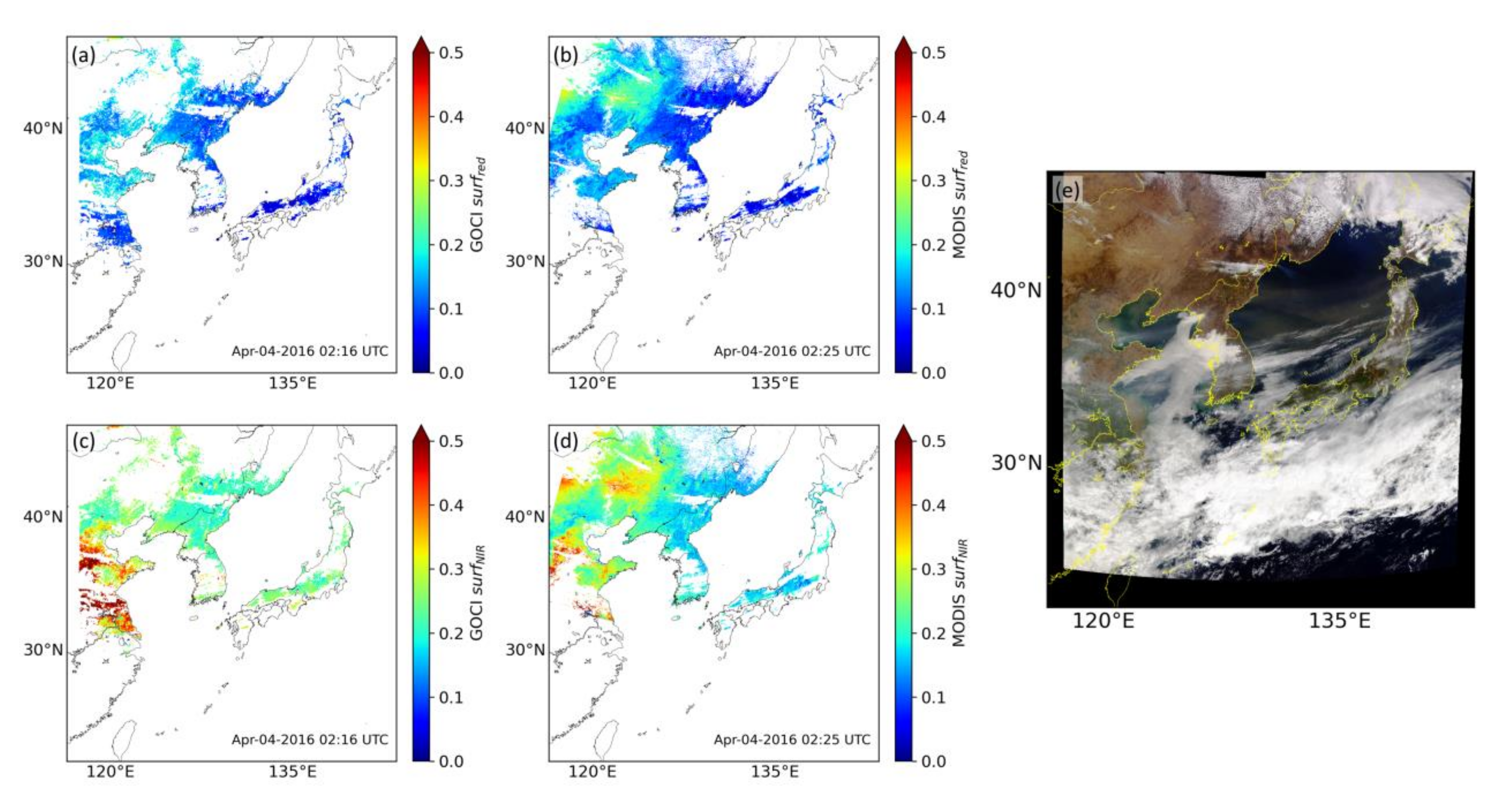
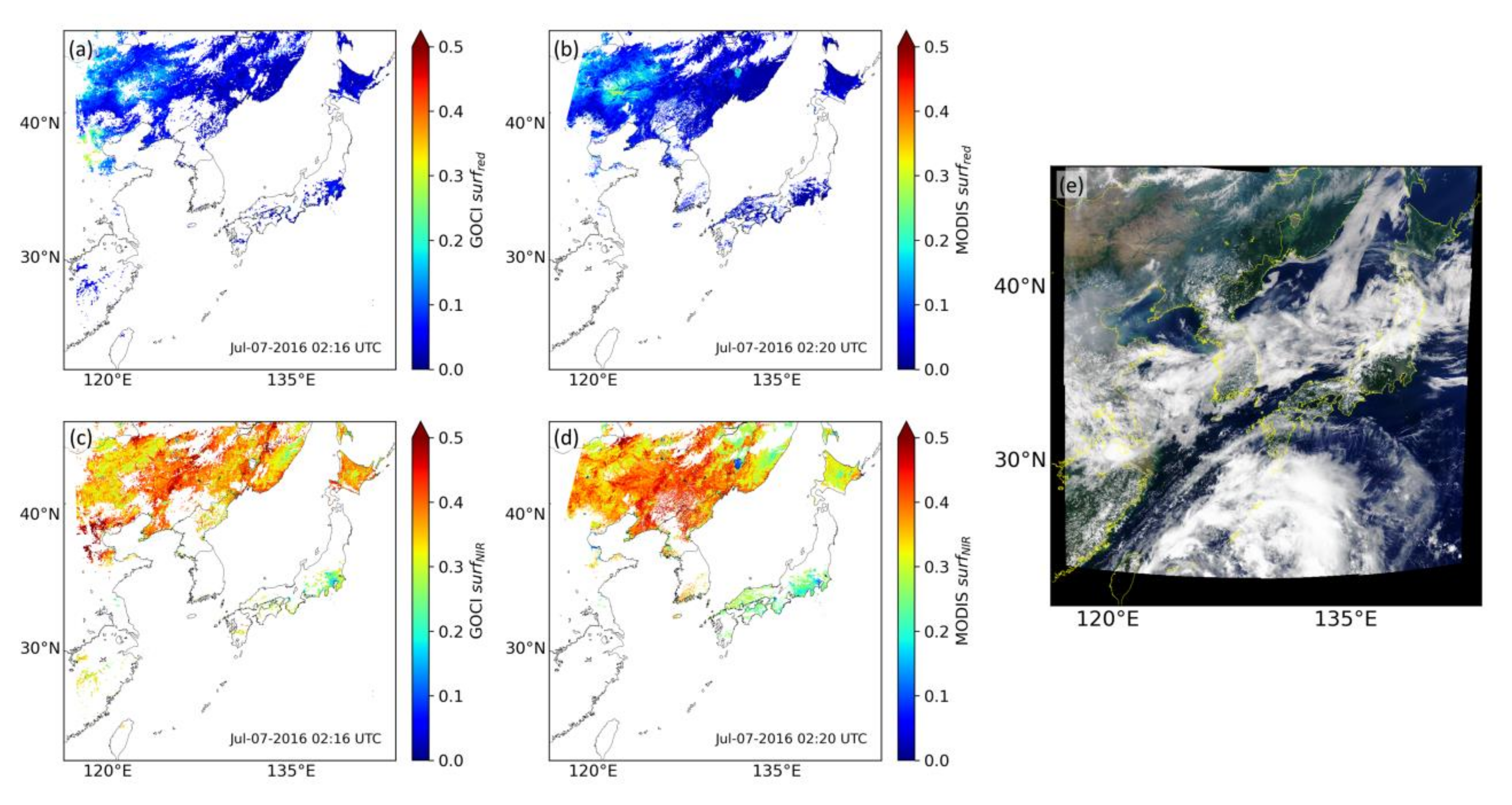
4.1. Qualitative Comparison with MODIS LSR Products

To evaluate the spatial consistency, we compared our results with operational MODIS LSR products. Quantitative comparison between LSRs from different satellites is limited because of LSR sensitivity to geometric conditions (SZA, VZA, and RAA), atmospheric conditions, and the spectral response of satellite-mounted sensors. Yeom et al. [79] found the RMSE between GOCI and MODIS LSRs as 0.11 and 0.134 for red and NIR bands, respectively, although they applied the semi-empirical BRDF model to remove surface anisotropy effects in the LSRs. This discrepancy may inevitably occur due to differences in methods and assumptions used within the algorithm [80]; therefore, we only performed a qualitative comparison. Figure 2 and Figure 3 show the geographical distributions of GOCI and MODIS LSRs at red (680 nm) and NIR (865 nm) channels for 9 April and 7 July 2016. Other bands also show similar results; however, they are excluded for brevity. Our results show comparable geographic distributions with MODIS at both red and NIR channels, although there are differences between GOCI and MODIS LSRs. The RMSEs of LSR at red (NIR) channels for 9 April and 7 July 2016, are 0.0458 (0.0554) and 0.0372 (0.0630), respectively, which agrees with the results of previous studies [79]. In addition, our results capture the changes in LSR with vegetation growth well. 9 April (Figure 2) corresponds to early spring, when vegetation begins to grow in northeastern China and Korean Peninsula. Conversely, 7 July (Figure 3) is the post-growth and corresponds to the maturity phase [81]. These phenological dynamics are well illustrated in RGB true-color images. Northeastern China and the Korean Peninsula with sparse vegetation cover are indicated as yellow ochre in Figure 2e. In contrast, they are shown as green in Figure 3e because of healthy vegetation cover. Because of this, the Figure 3 shows a higher GOCI LSR in the NIR band than the Figure 2, but a lower LSR in the red band. These results demonstrate that GOCI LSR can effectively reflect changes according to the state of the land surface; thus, it can be used for land surface monitoring.

However, GOCI and MODIS use different cloud masks; thus, their LSR spatial distribution is different. In particular, both dates contained a few clouds in the RGB True Color image, but GOCI was unable to retrieve the LSR on the bright land surface of Mongolia. This limitation may be caused by the uncertainty of cloud masking due to the absence of Infrared channels in GOCI. GOCI-II will be able to overcome this limitation by using the AMI cloud mask product, which can cover the temporal and spatial coverages of GOCI-II with reliable accuracy (the probability of detection and false alarm ratio of the AMI cloud mask are 92% and 13%, respectively [82]).

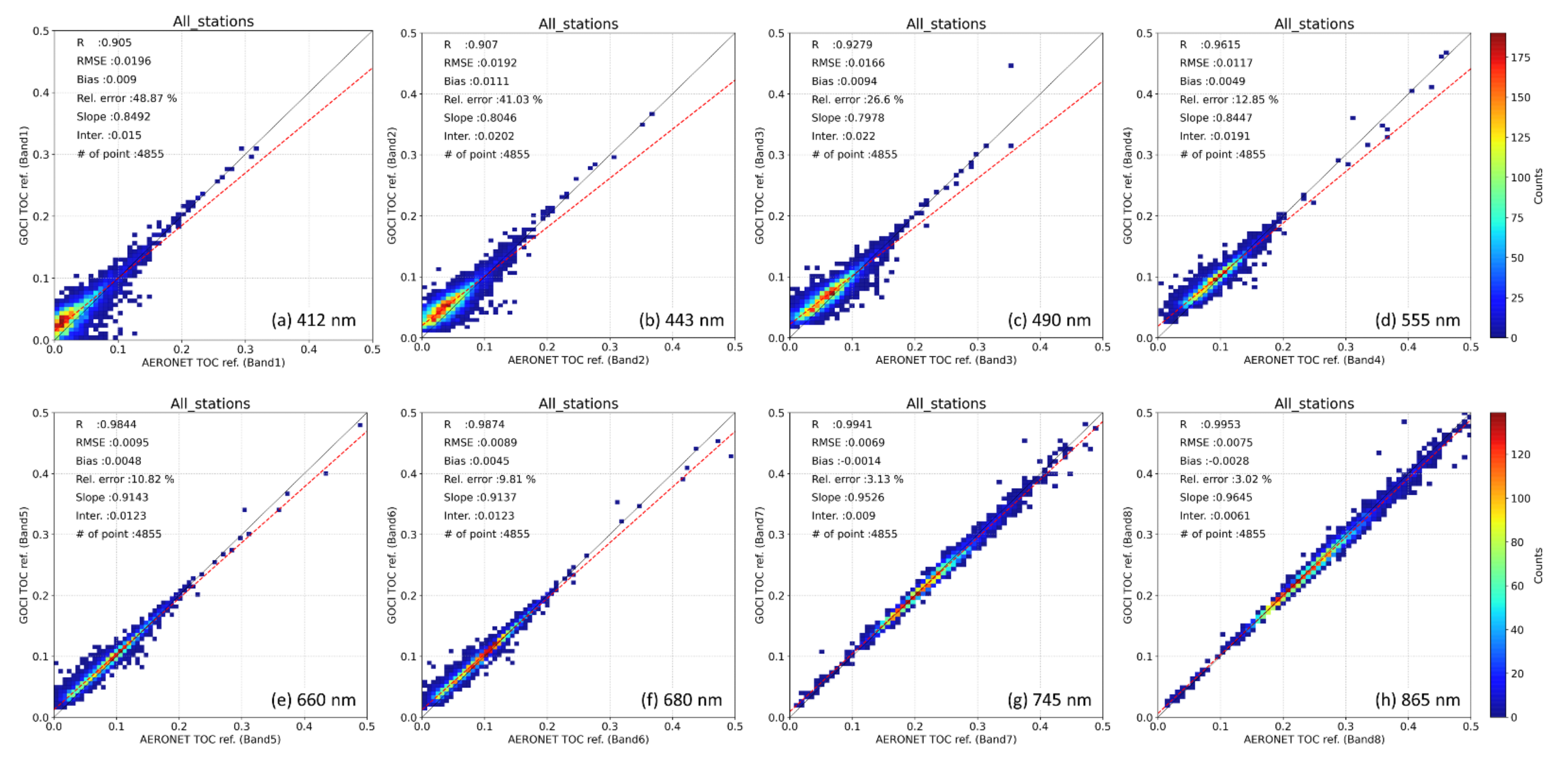
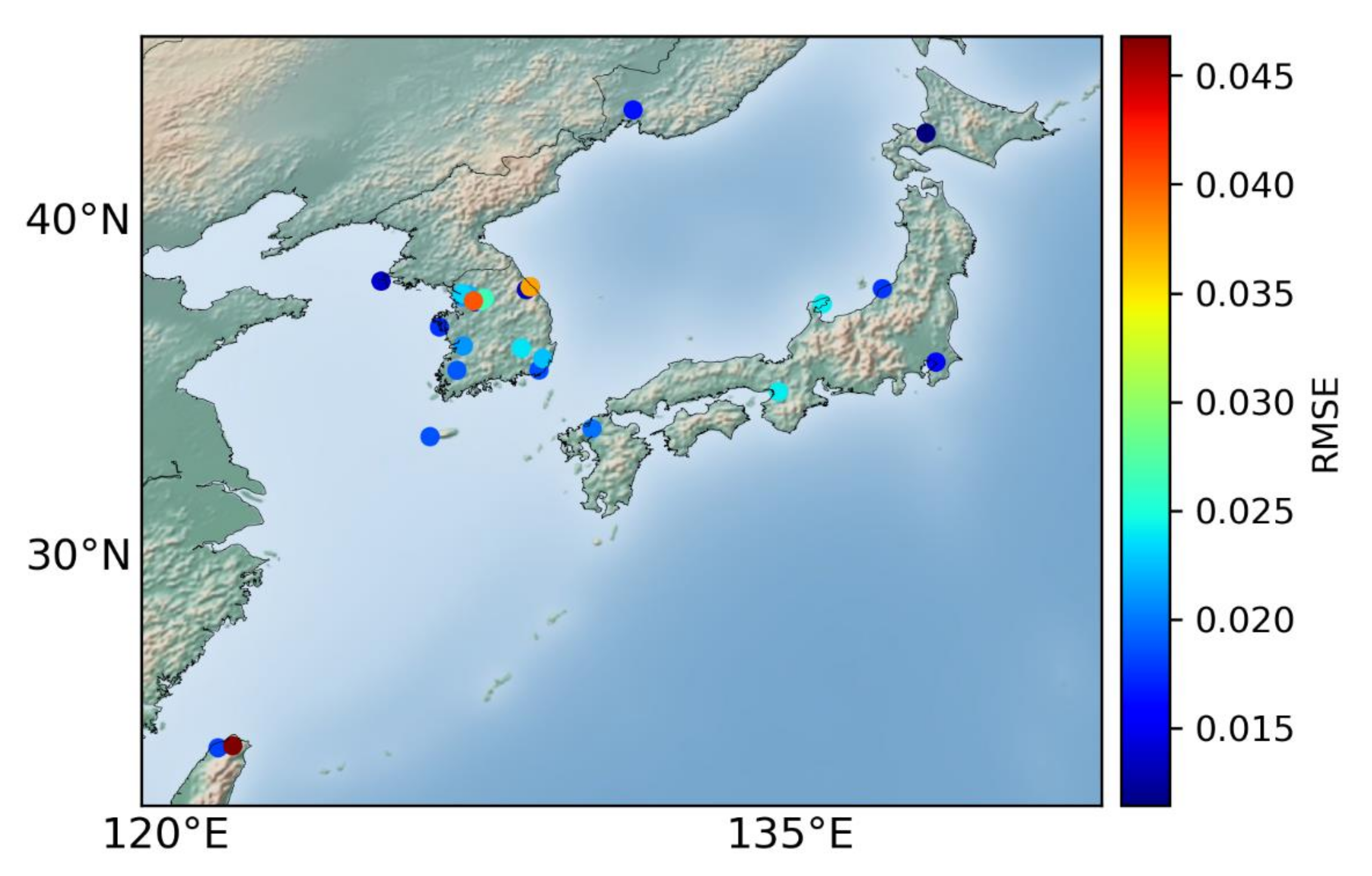
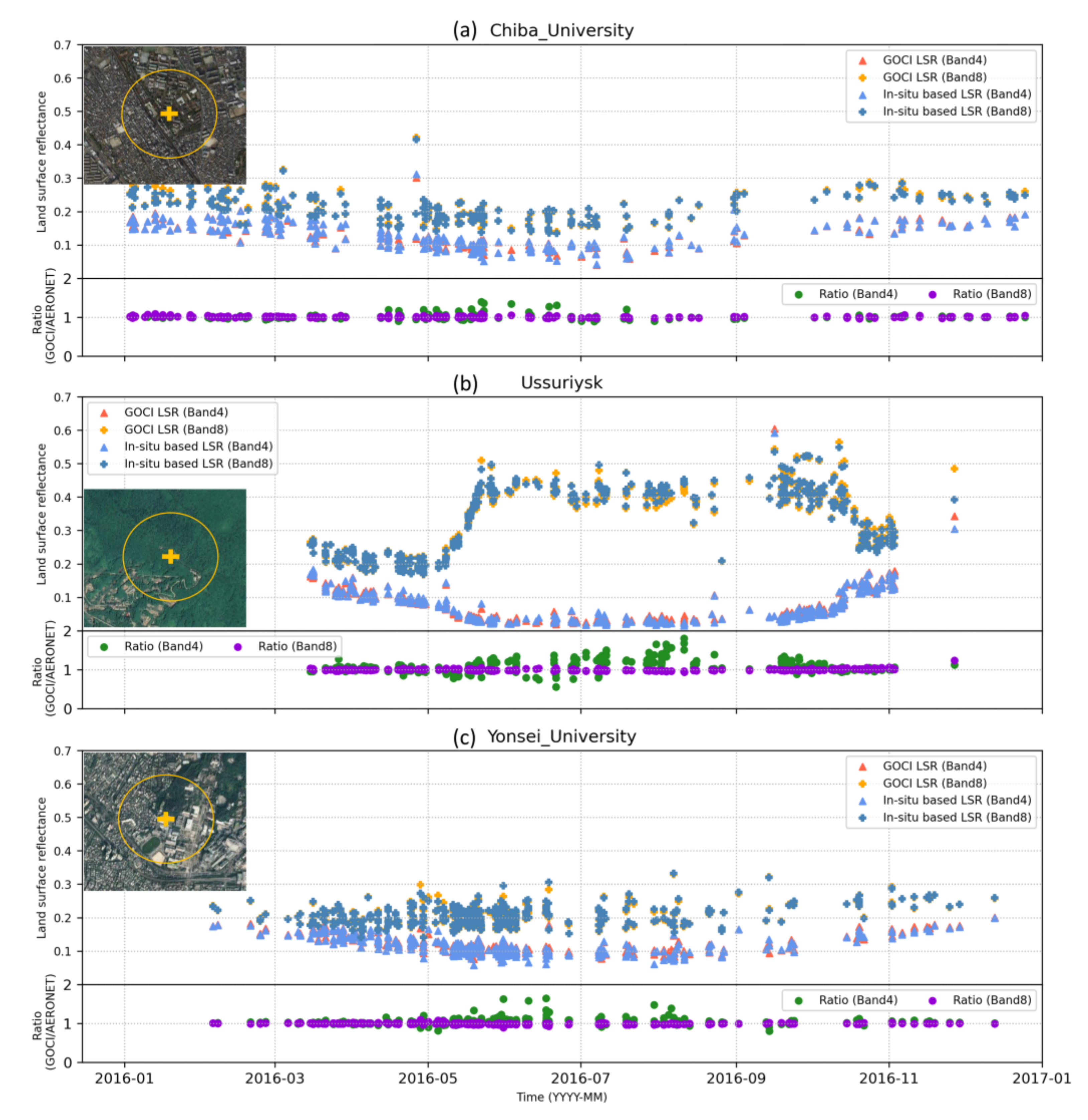
4.2. Validation with Reference LSR

For quantitative evaluation of estimated GOCI LSR, we compared our results with in situ reference LSR. In this analysis, 4855 matchup pairs were used. Figure 4 shows the scatterplot between the GOCI LSR and in situ reference LSR for each channel. Our results show good agreement compared to the reference data set with RMSE less than 0.02, R greater than 0.9, and bias less than ±0.01 for all channels. With decreasing central wavelength, the RMSE slightly increases (from 0.0075 at 865 nm to 0.0196 at 412 nm), while the relative error (percentage ratio of RMSE to mean LSR) significantly increases (from 3.02% at 865 nm to 48.87% at 412 nm). In addition, in the Band 1 to 3, points are distributed far from the one-to-one correspondence line. The biases of bands 1 and 2 are 0.009 and 0.0111, respectively, while the biases of bands 7 and 8 are −0.0014 and −0.0028, respectively. Because of this discrepancy, the slope of regression lines for VIS bands is less than the slope for NIR bands, but the intercept is greater. This trend was similar to the results of the ABI LSR validation [35] and was assumed to be related to the greater atmospheric effects (particularly the effects of aerosols) at shorter wavelengths [83]. Figure 5 shows RMSE of LSR in Band 1 compared to in-situ reference LSR for each station. The RMSE ranges from 0.0115 to 0.04682 and is lower than 0.0266 at most stations (25 stations). Only three sites (DRAGON_GangneungWNU, DRAGON_Hankuk_UFS, and Taipei_CWB), colored orange to dark red in Figure 5, show RMSEs of over 0.03. However, these sites had very small matchup pairs (2, 21, and 6, respectively), considering that the total number of matchup pairs was 4855. There is no significant relationship between RMSE and geospatial locations of AERONET stations. The remaining GOCI bands (2–8) exhibited similar results; however, they were excluded for simplicity.

Figure 6 presents the time series of GOCI LSR and in situ reference LSR in red and NIR bands for three stations (Chiba University, Ussuriysk, and Yonsei University), which have different land covers. For all three sites, GOCI LSR agreed well with in situ reference LSR for bands 4 and 8. In addition, the ratio of GOCI LSR to in situ reference LSR in the near-infrared band showed a relatively stable time series close to 1, but showed relatively large variability in the red band. As mentioned earlier, the large variability in the red band was regarded to be due to the greater influence of the atmosphere and lower magnitude of reflectance. Our results also well indicate the seasonal variation of LSR in different land types. Chiba University is located at a downtown site in Japan and the surrounding 500 m radius is mainly composed of man-made structures and asphalt (Figure 6a); thus, GOCI LSR shows little temporal variability in LSR for both bands 4 and 8 throughout 2016. GOCI LSR decreases until summer when SZA gradually reduced. On the contrariwise, since September 2016, GOCI LSR increases with increasing SZA. This result indicates that GOCI LSR well expresses the seasonal change in LSR according to SZA. Ussuriysk is located in Russia and, as shown in its RGB true color images (Figure 6b), it is surrounded by vegetation cover. Therefore, its LSR is dominantly affected by the spectral characteristics of vegetation. In practice, GOCI LSRs in band 4 and 8 have shown typical vegetation reflectance (high NIR and low Visible) during the vegetation growing season (May to November). A 500 m radius of the Yonsei University site includes both man-made structures and some vegetation (Figure 6c). Therefore, the vegetation cover partially affects the LSR of this site. In this site, the GOCI LSR showed a temporal change similar to that of Chiba University. However, in response to the spectral characteristics of vegetation, GOCI and in situ LSR of band 8 were slightly increased, unlike Chiba University. The results of time-series analysis also indicated that GOCI LSR well expresses the change in LSR according to land type and phylogeny.

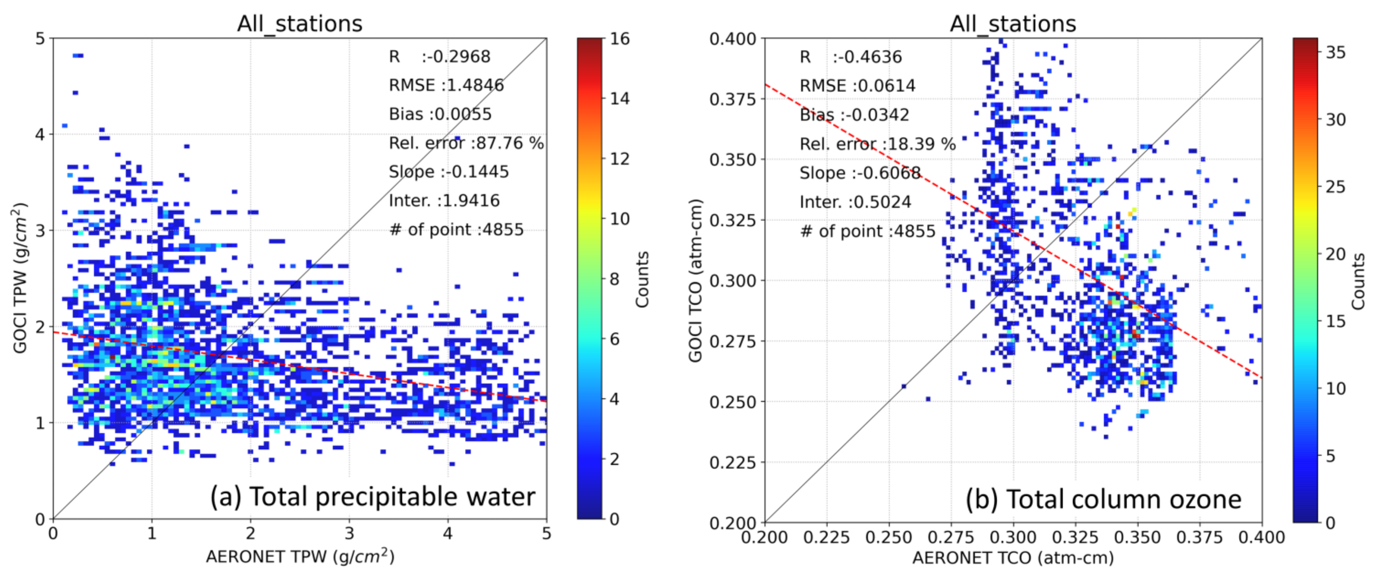
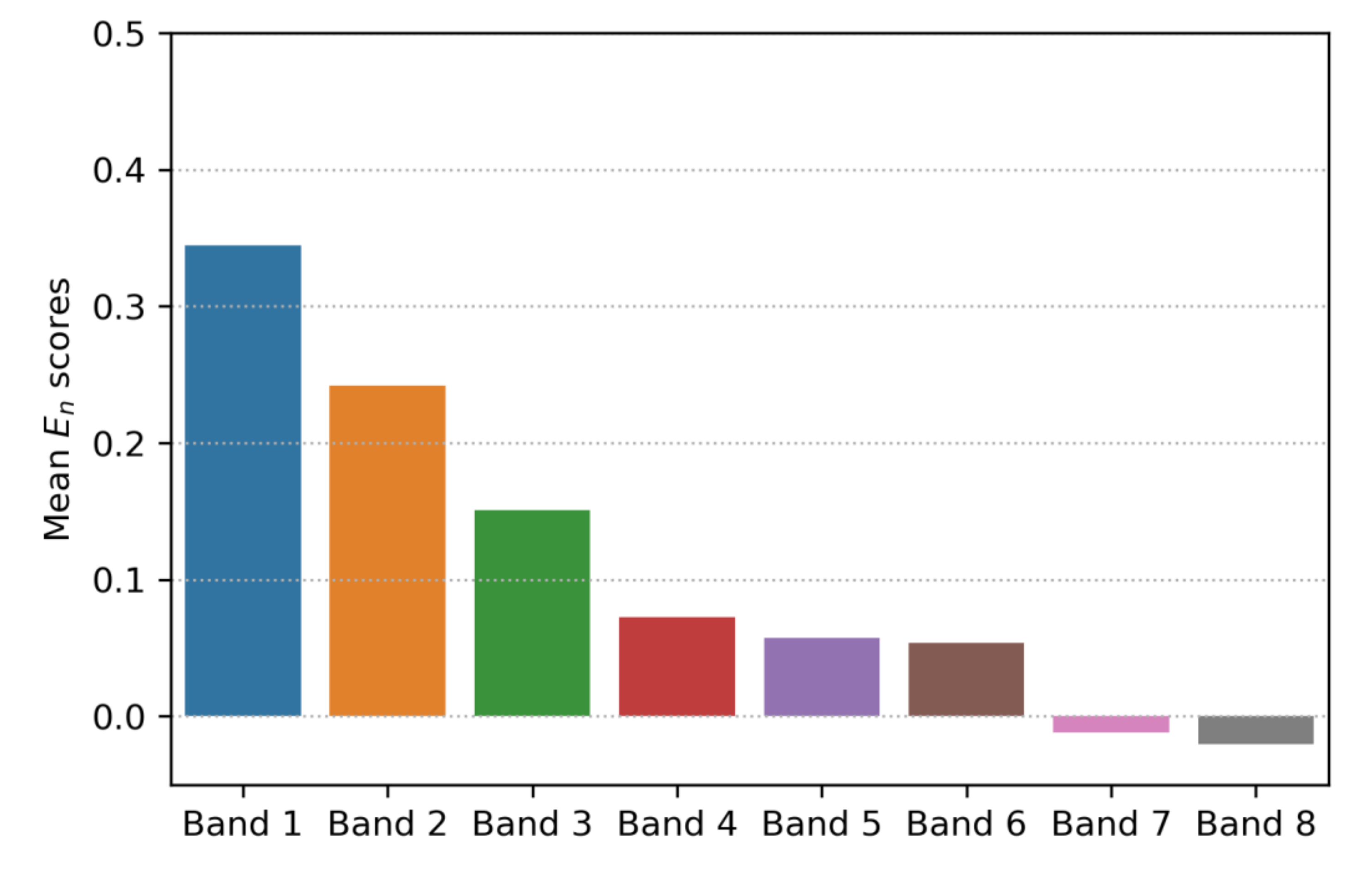
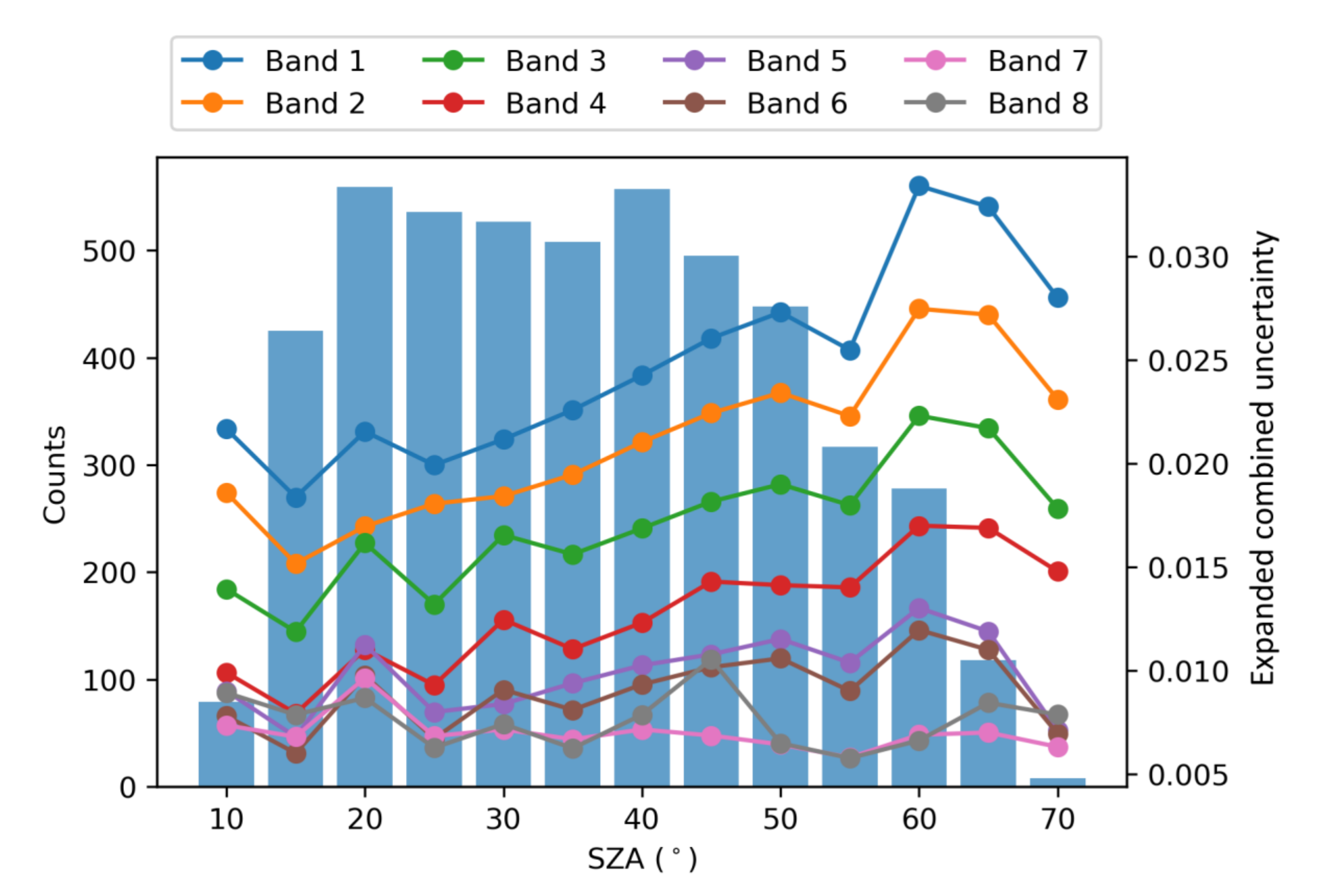
4.3. Uncertanties Introduced by Input Parameters

To estimate the uncertainty in LSR, the uncertainties in CAMS TPW and TCO were derived by comparing CAMS data with AERONET measurements. Figure 7 shows the validation results of CAMS TPW and TCO. For both TPW and TCO, CAMS data showed poor agreement with AERONET measurements. Each point was far from the diagonal and appeared to be randomly distributed, with R values of −0.2968 and −0.4636 for TPW and TCO, respectively. The RMSEs were 1.4846 and 0.0614 for TPW and TCO, respectively, and biases were 0.0055 and −0.0345, respectively. This error may be due to the low spatial resolution (0.125°) and temporal resolution (daily) of the CAMS. To estimate the uncertainty in LSR retrieval introduced by this discrepancy, the uncertainties in TPW and TCO were set as 87.76% and 18.39%, respectively, which are the relative errors. The uncertainty in AOD was determined from a previous study [51].

Table 4. Uncertainties introduced by AOD, TPW, and TCO, and total combined uncertainty in LSR. The numbers in parentheses indicate the contribution degree (percentage) of each input parameter to the total uncertainty in LSR.

Input Parameter	Band 1 (412 nm)	Band 2 (443 nm)	Band 3 (490 nm)	Band 4 (555 nm)	Band 5 (660 nm)	Band 6 (680 nm)	Band 7 (745 nm)	Band 8 (865 nm)
AOD	0.0240 (100%)	0.0205 (97.5%)	0.0165 (83.4%)	0.0112 (67.6%)	0.0096 (70.0%)	0.0088 (75.6%)	0.0054 (48.4%)	0.0068 (65.3%)
TPW	0 (0%)	0 (0%)	0 (0%)	0.0001 (0.7%)	0.0021 (15.5%)	0.0004 (3.2%)	0.0046 (40.9%)	0.0036 (34.7%)
TCO	0 (0%)	0.0005 (2.5%)	0.0033 (16.6%)	0.0053 (31.7%)	0.0020 (14.5%)	0.0025 (21.2%)	0.0012 (10.7%)	0 (0%)
$\mathrm{Total} \mathrm{uncerainty}$	0.0240	0.0205	0.0168	0.0124	0.0100	0.0091	0.0072	0.0077

presents the total combined uncertainty in estimated LSR ($u_{LSR}$) caused by input parameters, calculated using Equation (11). The $u_{LSR}$ values of bands 1 to 8 ranged from 0.0072 to 0.0240 and generally decreased as the central wavelength increases. The results were similar to the results presented in Figure 4. The uncertainty component of AOD significantly contributed to the $u_{LSR}$ (over 48% for all channels). Thus, AOD contributions in the visible spectrum (100%, 97.54%, 83.44%, 67.64%, 69.98%, 75.64% for channels 1–6, respectively) were higher than the contributions in the NIR spectrum (48.64 and 65.30% for bands 7 and 8, respectively). The uncertainties in TPW in bands 1–3 hardly affected the $u_{LSR}$, but bands 5, 7, and 8 showed a relatively high contribution to uncertainty (15.5%, 40.94%, and 34.70%, respectively). The contribution of uncertainty in TCO to $u_{LSR}$ also varies with central wavelength. Band 4 shows the greatest contribution (33.16%), while bands 1 and 8 show no contribution. The spectral-dependent uncertainty was related to the spectral characteristics of each atmospheric component. In addition, the absolute value of uncertainty in LSR due to the error of TPW and TCO is low. This is consistent with the results of previous studies [33]. The percentage ratio of the TPW-induced uncertainty in LSR to the mean reference LSR in band 7 is only 2%. It was reasonable considering the high uncertainty in TPW (87.76%). The $u_{LSR}$ for bands 3–8 could be able to reduce by using AMI TPW and GEMS TCO. These products have higher temporal and spatial resolutions than CAMS near-real-time products; thus, they allow for more realistic representations of the spatial and temporal variations of atmospheric compositions. Figure 8 shows the mean $E_n$ scores for GOCI channels. Similar to the previous results, the $E_n$ score tends to increase as the center wavelength decreases. However, $E_n$ shows range between −1 to 1 for all channels (0.35 for band 1 and −0.02 for band 8). This result was pointed out that GOCI LSR has good agreement with reference LSR, and the uncertainty of GOCI LSR derived from this study was valid.

Figure 9 presents the $u_{LSR}$ of eight GOCI bands depending on SZA, which was one of the variables that greatly influence uncertainty in LSR. The $u_{LSR}$ increased with decreasing central wavelength. For the VIS bands (1–6), as SZA increases, the $u_{LSR}$ increased (the regression line slopes for bands 1–6 are 0.00021, 0.00017, 0.00013, 0.00013, 0.00004, and 0.00004, respectively). In band 1, the maximum $u_{LSR}$ is 0.0324, corresponding to an SZA of 60°. The large decrease in uncertainty at SZA above 60° may be related to the small amount of data. In the two NIR bands (7 and 8), the slope of the regression line was close to 0, and the variation of the $u_{LSR}$ with SZA was not shown. For all GOCI bands and SZA, the $u_{LSR}$ was less than 0.04. These results indicated that the estimated GOCI LSR has reasonable uncertainty for most observation conditions [84].

5. Conclusions

We developed an LSR retrieval algorithm for GOCI-II operation and describe the input data-induced uncertainty in estimated LSR. We estimated LSR using the absolute atmospheric correction method because of its atmospheric effect simulation accuracy under various geometric, atmospheric, and spectral conditions, although prior information was needed. We used the 6SV LUT, which was constructed via comprehensive RTM calculation. Moreover, we used the 6D interpolation method to avoid the errors of intervals associated with the 6SV LUT. The cloud mask and AOD, which are important variables for LSR retrieval from satellite-mounted sensor measurements, were obtained from operational GOCI AOD algorithms. CAMS TPW and TCO data were selected as atmospheric input data in our algorithm. Despite their lower resolutions than GOCI data, they are suitable, as they do not have high sensitivity in LSR estimation.

The estimated GOCI LSR mostly agreed well with MODIS LSR for vegetation growth and post-vegetation growth periods. In some regions, especially that of a bright land surface in Mongolia, GOCI could not retrieve LSR, despite the clear-sky condition. This limitation is due to the GOCI channel configuration; the GOCI has only VIS to NIR channels and thus is limited in discriminating clouds and bright surfaces. This problem can be overcome using an AMI cloud mask when applying the proposed algorithm with GOCI-II. The results also agreed well with in situ reference LSR, with a high R of over 0.9 and low RMSE of less than 0.02 for all channels. All sites except three (which had fewer observations) showed reliable RMSEs. Among the GOCI eight bands, band 1 showed the highest RMSE (0.0115–0.0266). In addition, time-series analysis showed that GOCI LSR well expressed seasonal variation according to changes in SZA and the phenological dynamics of vegetation. In all bands, AOD contributed the most to uncertainty in LSR. TPW and TCO data also affected uncertainty in LSR for certain spectral channels. Data with improved spatiotemporal resolution and accuracy, such as AMI products, are needed to reduce the CAMS TPW- and TCO-induced errors in GOCI LSR. Nevertheless, the estimated GOCI LSR showed reasonable uncertainty (<0.04) even under high SZA (≥70°) conditions.

Our proposed algorithm can be used with GOCI-II, and it can provide data for analysis of changes in land surface, land use [85], and phenological dynamics [86], with a high spatial resolution of 250 m and hourly temporal resolution. In addition, the algorithm can provide continuous and sustained LSR products from the GOCI series for Northeast Asia that can be applied to climate change studies. In this study, the uncertainty in LSR retrieval caused by the uncertainty of the input parameter was analyzed, but this is cannot interpret the uncertainty of methods used in this study. Since the assumptions used in the 6SV simulation (e.g., fixed atmospheric profile and Lambertian assumption) are not always valid, further uncertainty analysis should be performed in future studies for robust uncertainty analysis. In addition, for more reliable assessment, additional validation exercises should be performed using directly measured in-situ LSR and high-resolution satellite-based LSR products.

References

1. Raiyani, K.; Gonçalves, T.; Rato, L.; Salgueiro, P.; Marques da Silva, J.R. Sentinel-2 Image Scene Classification: A Comparison between Sen2Cor and a Machine Learning Approach. Remote Sens. 2021, 13, 300. [Google Scholar] [CrossRef]
2. Nath, B.; Ni-Meister, W. The Interplay between Canopy Structure and Topography and Its Impacts on Seasonal Variations in Surface Reflectance Patterns in the Boreal Region of Alaska—Implications for Surface Radiation Budget. Remote Sens. 2021, 13, 3108. [Google Scholar] [CrossRef]
3. Shih, H.; Stow, D.A.; Tsai, Y.; Roberts, D.A. Estimating the Starting Time and Identifying the Type of Urbanization Based on Dense Time Series of Landsat-Derived Vegetation-Impervious-Soil (V-I-S) Maps—A Case Study of North Taiwan from 1990 to 2015. Int. J. Appl. Earth Obs. Geoinf. 2020, 85, 101987. [Google Scholar] [CrossRef]
4. Jin, D.; Chung, S.-R.; Lee, K.-S.; Seo, M.; Choi, S.; Seong, N.-H.; Jung, D.; Sim, S.; Kim, J.; Han, K.-S. Development of Geo-KOMPSAT-2A Algorithm for Sea-Ice Detection Using Himawari-8/AHI Data. Remote Sens. 2020, 12, 2262. [Google Scholar] [CrossRef]
5. Sahu, B.S.; Maharana, P.; Tandon, A.; Attri, A.K. Surface Reflectance Change Can Induce Reduction in the Surrounding Ambient Environment Warming. JCC 2021, 7, 63–72. [Google Scholar] [CrossRef]
6. Painter, T.H.; Bryant, A.C.; Skiles, S.M. Radiative Forcing by Light Absorbing Impurities in Snow from MODIS Surface Reflectance Data: RADIATIVE FORCING BY IMPURITIES IN SNOW. Geophys. Res. Lett. 2012, 39. [Google Scholar] [CrossRef]
7. Potapov, P.; Hansen, M.C.; Kommareddy, I.; Kommareddy, A.; Turubanova, S.; Pickens, A.; Adusei, B.; Tyukavina, A.; Ying, Q. Landsat Analysis Ready Data for Global Land Cover and Land Cover Change Mapping. Remote Sens. 2020, 12, 426. [Google Scholar] [CrossRef] [Green Version]
8. Hilker, T. Surface Reflectance/Bidirectional Reflectance Distribution Function. In Comprehensive Remote Sensing; Elsevier: Cham, Switzerland, 2018; pp. 2–8. ISBN 9780128032213. [Google Scholar]
9. Doxani, G.; Vermote, E.; Roger, J.-C.; Gascon, F.; Adriaensen, S.; Frantz, D.; Hagolle, O.; Hollstein, A.; Kirches, G.; Li, F.; et al. Atmospheric Correction Inter-Comparison Exercise. Remote Sens. 2018, 10, 352. [Google Scholar] [CrossRef] [Green Version]
10. Thompson, D.R.; Natraj, V.; Green, R.O.; Helmlinger, M.C.; Gao, B.-C.; Eastwood, M.L. Optimal Estimation for Imaging Spectrometer Atmospheric Correction. Remote Sens. Environ. 2018, 216, 355–373. [Google Scholar] [CrossRef]
11. Jiménez-Muñoz, J.C.; Sobrino, J.A.; Mattar, C.; Franch, B. Atmospheric Correction of Optical Imagery from MODIS and Reanalysis Atmospheric Products. Remote Sens. Environ. 2010, 114, 2195–2210. [Google Scholar] [CrossRef]
12. Mahiny, A.S.; Turner, B.J. A Comparison of Four Common Atmospheric Correction Methods. Photogramm Eng. Remote Sens. 2007, 73, 361–368. [Google Scholar] [CrossRef]
13. Sriwongsitanon, N.; Surakit, K.; Thianpopirug, S. Influence of Atmospheric Correction and Number of Sampling Points on the Accuracy of Water Clarity Assessment Using Remote Sensing Application. J. Hydrol. 2011, 401, 203–220. [Google Scholar] [CrossRef]
14. Ariza, A.; Robredo Irizar, M.; Bayer, S. Empirical Line Model for the Atmospheric Correction of Sentinel-2A MSI Images in the Caribbean Islands. Eur. J. Remote Sens. 2018, 51, 765–776. [Google Scholar] [CrossRef]
15. Wang, T.; Du, L.; Yi, W.; Hong, J.; Zhang, L.; Zheng, J.; Li, C.; Ma, X.; Zhang, D.; Fang, W.; et al. An Adaptive Atmospheric Correction Algorithm for the Effective Adjacency Effect Correction of Submeter-Scale Spatial Resolution Optical Satellite Images: Application to a WorldView-3 Panchromatic Image. Remote Sens. Environ. 2021, 259, 112412. [Google Scholar] [CrossRef]
16. Chrysoulakis, N.; Abrams, M.; Feidas, H.; Arai, K. Comparison of Atmospheric Correction Methods Using ASTER Data for the Area of Crete, Greece. Int. J. Remote Sens. 2010, 31, 6347–6385. [Google Scholar] [CrossRef]
17. Wang, Y.; Liu, L.; Hu, Y.; Li, D.; Li, Z. Development and Validation of the Landsat-8 Surface Reflectance Products Using a MODIS-Based per-Pixel Atmospheric Correction Method. Int. J. Remote Sens. 2016, 37, 1291–1314. [Google Scholar] [CrossRef]
18. Rahman, H.; Dedieu, G. SMAC: A Simplified Method for the Atmospheric Correction of Satellite Measurements in the Solar Spectrum. Int. J. Remote Sens. 1994, 15, 123–143. [Google Scholar] [CrossRef]
19. Cooley, T.; Anderson, G.P.; Felde, G.W.; Hoke, M.L.; Ratkowski, A.J.; Chetwynd, J.H.; Gardner, J.A.; Adler-Golden, S.M.; Matthew, M.W.; Berk, A.; et al. FLAASH, a MODTRAN4-Based Atmospheric Correction Algorithm, Its Application and Validation. In Proceedings of the IEEE International Geoscience and Remote Sensing Symposium, Toronto, ON, Canada, 24–28 June 2002; Volume 3, pp. 1414–1418. [Google Scholar]
20. Jha, S.S.; Manohar Kumar, C.V.S.S.; Nidamanuri, R.R. Flexible Atmospheric Compensation Technique (FACT): A 6S Based Atmospheric Correction Scheme for Remote Sensing Data. Geocarto Int. 2021, 36, 28–46. [Google Scholar] [CrossRef]
21. Santini, F.; Palombo, A. Physically Based Approach for Combined Atmospheric and Topographic Corrections. Remote Sens. 2019, 11, 1218. [Google Scholar] [CrossRef] [Green Version]
22. Palombo, A.; Santini, F. ImaACor: A Physically Based Tool for Combined Atmospheric and Topographic Corrections of Remote Sensing Images. Remote Sens. 2020, 12, 2076. [Google Scholar] [CrossRef]
23. Guanter, L.; Del Carmen, M.; Sanpedro, G.; Moreno, J. A method for the atmospheric correction of ENVISAT/MERIS data over land targets. Int. J. Remote Sens. 2007, 28, 709–728. [Google Scholar] [CrossRef]
24. Guanter, L.; Richter, R.; Kaufmann, H. On the application of the MODTRAN4 atmospheric radiative transfer code to optical remote sensing. Int. J. Remote Sens. 2009, 30, 1407–1424. [Google Scholar] [CrossRef]
25. Sanders, L.C.; Schott, J.R.; Raqueno, R. A VNIR/SWIR atmospheric correction algorithm for hyperspectral imagery with adjacency effect. Remote Sens. Environ. 2001, 78, 252–263. [Google Scholar] [CrossRef]
26. Ilori, C.O.; Pahlevan, N.; Knudby, A. Analyzing Performances of Different Atmospheric Correction Techniques for Landsat 8: Application for Coastal Remote Sensing. Remote Sens. 2019, 11, 469. [Google Scholar] [CrossRef] [Green Version]
27. Vermote, E.F.; Vermeulen, A. MODIS ATBD: Atmospheric Correction Algorithm: Spectral Reflectances (MOD09), Version 4.0. 1999. Available online: http://modis.gsfc.nasa.gov/data/atbd/atbd_mod08.pdf (accessed on 10 November 2021).
28. Franch, P.B.; Roger, J.C.; Vermote, E.F. Suomi-NPP VIIRS Surface Reflectance Algorithm Theoretical Basis Document (ATBD), Version 2.0, 10 October 2016. Available online: https://viirsland.gsfc.nasa.gov/PDF/ATBD_VIIRS_SR_v2.pdf (accessed on 10 November 2021).
29. Liang, S.; Wang, D.; He, T. GOES-R Advanced Baseline Imager (ABI) Algorithm Theoretical Basis Document for Surface Albedo; NOAA NESDIS Center for Satellite Applications and Research: Washington, DC, USA, 2010. [Google Scholar]
30. Roujean, J.-L.; Leon-Tavares, J.; Smets, B.; Claes, P.; Camacho De Coca, F.; Sanchez-Zapero, J. Surface Albedo and Toc-r 300 m Products from PROBA-V Instrument in the Framework of Copernicus Global Land Service. Remote Sens. Environ. 2018, 215, 57–73. [Google Scholar] [CrossRef]
31. Carrer, D.; Moparthy, S.; Lellouch, G.; Ceamanos, X.; Pinault, F.; Freitas, S.; Trigo, I. Land Surface Albedo Derived on a Ten Daily Basis from Meteosat Second Generation Observations: The NRT and Climate Data Record Collections from the EUMETSAT LSA SAF. Remote Sens. 2018, 10, 1262. [Google Scholar] [CrossRef] [Green Version]
32. Lee, K.-S.; Chung, S.-R.; Lee, C.; Seo, M.; Choi, S.; Seong, N.-H.; Jin, D.; Kang, M.; Yeom, J.-M.; Roujean, J.-L.; et al. Development of Land Surface Albedo Algorithm for the GK-2A/AMI Instrument. Remote Sens. 2020, 12, 2500. [Google Scholar] [CrossRef]
33. Lee, C.S.; Yeom, J.M.; Lee, H.L.; Kim, J.-J.; Han, K.-S. Sensitivity Analysis of 6S-Based Look-up Table for Surface Reflectance Retrieval. Asia-Pac. J. Atmos. Sci. 2015, 51, 91–101. [Google Scholar] [CrossRef]
34. Vanhellemont, Q.; Ruddick, K. Atmospheric Correction of Metre-Scale Optical Satellite Data for Inland and Coastal Water Applications. Remote Sens. Environ. 2018, 216, 586–597. [Google Scholar] [CrossRef]
35. Zhang, H.; Wang, L.Y. Developing Land Surface Directional Reflectance and Albedo Products from Geostationary GOES-R and Himawari Data: Theoretical Basis, Operational Implementation, and Validation. Remote Sens. 2019, 11, 2655. [Google Scholar] [CrossRef] [Green Version]
36. Shuai, Y.; Tuerhanjiang, L.; Shao, C.; Gao, F.; Zhou, Y.; Xie, D.; Liu, T.; Liang, J.; Chu, N. Re-understanding of land surface albedo and related terms in satellite-based retrievals. Big Earth Data 2020, 4, 45–67. [Google Scholar] [CrossRef]
37. Wu, X.; Xiao, Q.; Wen, J.; You, D.; Hueni, A. Advances in Quantitative Remote Sensing Product Validation: Overview and Current Status. Earth-Sci. Rev. 2019, 196, 102875. [Google Scholar] [CrossRef]
38. Ma, Z.; Jia, G.; Schaepman, M.E.; Zhao, H. Uncertainty Analysis for Topographic Correction of Hyperspectral Remote Sensing Images. Remote Sens. 2020, 12, 705. [Google Scholar] [CrossRef] [Green Version]
39. Povey, A.C.; Grainger, R.G. Known and Unknown Unknowns: Uncertainty Estimation in Satellite Remote Sensing. Atmos. Meas. Tech. 2015, 8, 4699–4718. [Google Scholar] [CrossRef] [Green Version]
40. Ryu, J.-H.; Han, H.-J.; Cho, S.; Park, Y.-J.; Ahn, Y.-H. Overview of Geostationary Ocean Color Imager (GOCI) and GOCI Data Processing System (GDPS). Ocean Sci. J. 2012, 47, 223–233. [Google Scholar] [CrossRef]
41. Wang, M.; Ahn, J.-H.; Jiang, L.; Shi, W.; Son, S.; Park, Y.-J.; Ryu, J.-H. Ocean Color Products from the Korean Geostationary Ocean Color Imager (GOCI). Opt. Express 2013, 21, 3835. [Google Scholar] [CrossRef] [PubMed]
42. Brown, M.E.; Pinzon, J.E.; Didan, K.; Morisette, J.T.; Tucker, C.J. Evaluation of the Consistency of Long-Term NDVI Time Series Derived from AVHRR, SPOT-Vegetation, SeaWiFS, MODIS, and Landsat ETM+ Sensors. IEEE Trans. Geosci. Remote Sens. 2006, 44, 1787–1793. [Google Scholar] [CrossRef]
43. Sayer, A.M.; Hsu, N.C.; Bettenhausen, C.; Jeong, M.-J.; Holben, B.N.; Zhang, J. Global and Regional Evaluation of Over-Land Spectral Aerosol Optical Depth Retrievals from SeaWiFS. Atmos. Meas. Tech. 2012, 5, 1761–1778. [Google Scholar] [CrossRef] [Green Version]
44. Kim, S.; Ahn, D.-S.; Han, K.-S.; Yeom, J.-M. Improved Vegetation Profiles with GOCI Imagery Using Optimized BRDF Composite. J. Sens. 2016, 2016, 7165326. [Google Scholar] [CrossRef]
45. Ke, Y.; Im, J.; Lee, J.; Gong, H.; Ryu, Y. Characteristics of Landsat 8 OLI-Derived NDVI by Comparison with Multiple Satellite Sensors and in-Situ Observations. Remote Sens. Environ. 2015, 164, 298–313. [Google Scholar] [CrossRef]
46. Son, S.; Kim, J. Land Cover Classification Map of Northeast Asia Using GOCI Data. Korean J. Remote Sens. 2019, 35, 83–92. [Google Scholar] [CrossRef]
47. Kim, H.-W.; Yeom, J.-M.; Shin, D.; Choi, S.; Han, K.-S.; Roujean, J.-L. An Assessment of Thin Cloud Detection by Applying Bidirectional Reflectance Distribution Function Model-Based Background Surface Reflectance Using Geostationary Ocean Color Imager (GOCI): A Case Study for South Korea: Thin Cloud Detection Based on BRDF Model. J. Geophys. Res. Atmos. 2017, 122, 8153–8172. [Google Scholar] [CrossRef]
48. Yeom, J.M.; Roujean, J.L.; Han, K.S.; Lee, K.S.; Kim, H.W. Thin cloud detection over land using background surface reflectance based on the BRDF model applied to Geostationary Ocean Color Imager (GOCI) satellite data sets. Remote Sens. Environ. 2020, 239, 111610. [Google Scholar] [CrossRef]
49. Korea Ocean Satellite Center Home Page. Available online: http://kosc.kiost.ac.kr/index.nm?menuCd=3 (accessed on 26 November 2021).
50. National Ocean Satellite Center Home Page. Available online: http://www.khoa.go.kr/nosc/satellite/searchL2.do (accessed on 26 November 2021).
51. Choi, M.; Kim, J.; Lee, J.; Kim, M.; Park, Y.-J.; Holben, B.; Eck, T.F.; Li, Z.; Song, H.H. GOCI Yonsei aerosol retrieval version 2 products: An improved algorithm and error analysis with uncertainty estimation from 5-year validation over East Asia. Atmos. Meas. Tech. 2018, 11, 385–408. [Google Scholar] [CrossRef] [Green Version]
52. Zhang, W.; Xu, H.; Zhang, L. Assessment of Himawari-8 AHI Aerosol Optical Depth Over Land. Remote Sens. 2019, 11, 1108. [Google Scholar] [CrossRef] [Green Version]
53. Vermote, E.F.; Kotchenova, S.Y. MOD09 (Surface Reflectance) User’s Guide, Version 1.1. 2008. Available online: https://patarnott.com/satsens/pdf/MOD09_UserGuide_v1_2.pdf (accessed on 12 October 2021).
54. Inness, A.; Ades, M.; Agusti-Panareda, A.; Barré, J.; Benedictow, A.; Blechschmidt, A.M.; Dominguez, J.J. The CAMS reanalysis of atmospheric composition. Atmos. Chem. Phys. 2019, 19, 3515–3556. [Google Scholar] [CrossRef] [Green Version]
55. Koffi, E.N.; Bergamaschi, P. Evaluation of Copernicus Atmosphere Monitoring Service Methane Products; Joint Research Centre: Ispra, Italy, 2018. [Google Scholar]
56. Eskes, H.J.; Basart, S.; Benedictow, A.; Bennouna, Y.; Blechschmidt, A.M.; Chabrillat, S.; Cuevas, E.; Errera, Q.; Flentje, H.; Hansen, K.M.; et al. Observation Characterisation and Validation Methods Document. Copernicus Atmosphere Monitoring Service (CAMS) Report. 2019. Available online: https://atmosphere.copernicus.eu/sites/default/files/publications/CAMS84_2018SC1_D6.1.1-2021_observations_v6_0.pdf (accessed on 21 November 2021).
57. Holben, B.N.; Eck, T.F.; Slutsker, I.; Tanré, D.; Buis, J.P.; Setzer, A.; Vermote, E.; Reagan, J.A.; Kaufman, Y.J.; Nakajima, T.; et al. AERONET—A Federated Instrument Network and Data Archive for Aerosol Characterization. Remote Sens. Environ. 1998, 66, 1–16. [Google Scholar] [CrossRef]
58. Hao, Y.; Cui, T.; Singh, V.P.; Zhang, J.; Yu, R.; Zhang, Z. Validation of MODIS Sea Surface Temperature Product in the Coastal Waters of the Yellow Sea. IEEE J. Sel. Top. Appl. Earth Obs. Remote Sens. 2017, 10, 1667–1680. [Google Scholar] [CrossRef]
59. Vermote, E.F.; Tanré, D.; Deuzé, J.L.; Herman, M.; Morcrette, J.-J. Second Simulation of the Satellite Signal in the Solar Spectrum, 6S: An Overview. IEEE Trans. Geosci. Remote Sens. 1997, 35, 675–686. [Google Scholar] [CrossRef] [Green Version]
60. Vermote, E.; Tanré, D.; Deuzé, J.L.; Herman, M.; Morcrette, J.J.; Kotchenova, S.Y. Second Simulation of a Satellite Signal in the Solar Spectrum-Vector (6SV); 6S User Guide Version 3. Available online: http://6s.ltdri.org/files/tutorial/6S_Manual_Part_1.pdf (accessed on 22 December 2021).
61. Kotchenova, S.Y.; Vermote, E.F.; Levy, R.; Lyapustin, A. Radiative transfer codes for atmospheric correction and aerosol retrieval: Intercomparison study. Appl. Opt. 2008, 47, 2215–2226. [Google Scholar] [CrossRef] [Green Version]
62. Rusia, P.; Bhateja, Y.; Misra, I.; Moorthi, S.M.; Dhar, D. An Efficient Machine Learning Approach for Atmospheric Correction. J. Indian Soc. Remote Sens. 2021, 49, 2539–2548. [Google Scholar] [CrossRef]
63. Kim, M.; Heo, J.H.; Sohn, E.H. Atmospheric Correction of True-Color RGB Imagery with Limb Area-Blending Based on 6S and Satellite Image Enhancement Techniques Using Geo-Kompsat-2A Advanced Meteorological Imager Data. Asia Pac. J. Atmos. Sci. 2021, volume, 1–20. [Google Scholar] [CrossRef]
64. Lee, K.S.; Lee, C.S.; Seo, M.; Choi, S.; Seong, N.H.; Jin, D.; Yeom, J.M.; Han, K.S. Improvements of 6S Look-Up-Table Based Surface Reflectance Employing Minimum Curvature Surface Method. Asia Pac. J. Atmos. Sci. 2020, 3, 1–14. [Google Scholar] [CrossRef] [Green Version]
65. Wang, D.; Liang, S.; Zhou, Y.; He, T.; Yu, Y. A new method for retrieving daily land surface albedo from VIIRS data. IEEE Trans. Geosci. Remote Sens. 2017, 55, 1765–1775. [Google Scholar] [CrossRef]
66. Yan, X.; Luo, N.; Liang, C.; Zang, Z.; Zhao, W.; Shi, W. Simplified and Fast Atmospheric Radiative Transfer model for satellite-based aerosol optical depth retrieval. Atmos. Environ. 2020, 224, 117362. [Google Scholar] [CrossRef]
67. Hu, S.; Zhang, L.; Baig, M.H.A.; Tong, Q. Using MODTRAN4 to build up a general look-up-table database for the atmospheric correction of hyperspectral imagery. In Proceedings of the 2012 IEEE International Geoscience and Remote Sensing Symposium, Munich, Germany, 22–27 July 2012; pp. 2458–2461. [Google Scholar]
68. Börner, A.; Wiest, L.; Keller, P.; Reulke, R.; Richter, R.; Schaepman, M.; Schläpfer, D. SENSOR: A tool for the simulation of hyperspectral remote sensing systems. ISPRS J. Photogramm. 2001, 55, 299–312. [Google Scholar] [CrossRef]
69. Bréon, F.-M.; Vermote, E. Correction of MODIS surface reflectance time series for BRDF effects. Remote Sens. Environ. 2012, 125, 1–9. [Google Scholar] [CrossRef]
70. Vermote, E.; Roger, J.C.; Franch, B.; Skakun, S. LaSRC (Land Surface Reflectance Code): Overview, application and validation using MODIS, VIIRS, LANDSAT and Sentinel 2 data’s. In Proceedings of the IGARSS—IEEE International Geoscience and Remote Sensing Symposium, Valencia, Spain, 23–27 July 2018; pp. 8173–8176. [Google Scholar]
71. Wang, Y.; Lyapustin, A.I.; Privette, J.L.; Morisette, J.T.; Holben, B. Atmospheric correction at AERONET locations: A new science and validation data set. IEEE Trans. Geosci. Remote Sens. 2009, 47, 2450–2466. [Google Scholar] [CrossRef]
72. MODIS Land Team Home Page. Available online: https://modis-land.gsfc.nasa.gov/ValStatus.php?ProductID=MOD09 (accessed on 21 November 2021).
73. Satellite Agriculture & Land Surface Applications Home Page. Available online: https://salsa.umd.edu/rtcodes.html (accessed on 21 November 2021).
74. Carmon, N.; Thompson, D.R.; Bohn, N.; Susiluoto, J.; Turmon, M.; Brodrick, P.G.; Connelly, D.S.; Braverman, A.; Cawse-Nicholson, K.; Green, R.O.; et al. Uncertainty quantification for a global imaging spectroscopy surface composition investigation. Remote Sens. Environ. 2020, 251, 112038. [Google Scholar] [CrossRef]
75. Bhatia, N.; Iordache, M.D.; Stein, A.; Reusen, I.; Tolpekin, V.A. Propagation of uncertainty in atmospheric parameters to hyperspectral unmixing. Remote Sens. Environ. 2018, 204, 472–484. [Google Scholar] [CrossRef]
76. JCGM. Evaluation of Measurement Data—Guide to the Expression of Uncertainty in Measurement (Évaluation des Données de Mesure—Guide pour L’expression de L’incertitude de Mesure.). Int. Organ. Stand. Geneva 2008, 50, 134. [Google Scholar]
77. Rydberg, B.; Eriksson, P.; Buehler, S.A.; Murtagh, D.P. Non-Gaussian Bayesian retrieval of tropical upper tropospheric cloud ice and water vapour from Odin-SMR measurements. Atmos. Meas. Tech. 2009, 2, 621–637. [Google Scholar] [CrossRef] [Green Version]
78. ISO. Statistical Methods for Use in Proficiency Testing by Inter-Laboratory Comparison; ISO 13528:2015(E); ISO: Geneva, Switzerland, 2015; Available online: https://www.iso.org/obp/ui/#iso:std:iso:13528:ed-2:v2:en (accessed on 23 December 2021).
79. Yeom, J.-M.; Kim, H.-O. Comparison of NDVIs from GOCI and MODIS Data towards Improved Assessment of Crop Temporal Dynamics in the Case of Paddy Rice. Remote Sens. 2015, 7, 11326–11343. [Google Scholar] [CrossRef] [Green Version]
80. Meroni, M.; Atzberger, C.; Vancutsem, C.; Gobron, N.; Baret, F.; Lacaze, R.; Eerens, H.; Leo, O. Evaluation of agreement between space remote sensing SPOT-VEGETATION fAPAR time series. IEEE Trans. Geosci. Remote Sens 2012, 51, 1–12. [Google Scholar] [CrossRef]
81. Lim, C.H.; An, J.H.; Jung, S.H.; Nam, G.B.; Cho, Y.C.; Kim, N.S.; Lee, C.S. Ecological consideration for several methodologies to diagnose vegetation phenology. Ecol. Res. 2018, 33, 363–377. [Google Scholar] [CrossRef]
82. National Meteorological Satellite Center Home Page. Available online: https://nmsc.kma.go.kr/homepage/html/base/cmm/selectPage.do?page=static.edu.atbdGk2a (accessed on 20 November 2021).
83. Lee, J.; Kim, J.; Song, C.H.; Ryu, J.-H.; Ahn, Y.-H.; Song, C. Algorithm for retrieval of aerosol optical properties over the ocean from the geostationary ocean color imager. Remote Sens. Environ. 2010, 114, 1077–1088. [Google Scholar] [CrossRef]
84. Claverie, M.; Vermote, E.F.; Franch, B.; Masek, J.G. Evaluation of the Landsat-5 TM and Landsat-7 ETM+ surface reflectance products. Remote Sens. Environ. 2015, 169, 390–403. [Google Scholar] [CrossRef]
85. Treitz, P.; Rogan, J. Remote sensing for mapping and monitoring land-cover and land-use change—An introduction. Prog. Plan. 2004, 61, 269–279. [Google Scholar] [CrossRef]
86. Liu, Y.; Wu, C.; Peng, D.; Xu, S.; Gonsamo, A.; Jassal, R.S.; Altaf Arain, M.; Lu, L.; Fang, B.; Chen, J.M. Improved modeling of land surface phenology using MODIS land surface reflectance and temperature at evergreen needleleaf forests of central North America. Remote Sens. Environ. 2016, 176, 152–162. [Google Scholar] [CrossRef]
Figure 1. RGB true-color images of study area on 02:16 UTC, 20 September 2016. R, G, and B correspond to GOCI bands 2 (443 nm), 3 (555), and 6 (680 nm), respectively.
Remotesensing 14 00360 g001
Figure 2. LSRs of red (680 nm) and NIR bands (865 nm) for GOCI (a,c) and MODIS (b,d); (e) GOCI RGB true-color image on 02:16 UTC, 9 April 2016. The times in (ad) are observation times.
Remotesensing 14 00360 g002
Figure 3. Same as Figure 2, but for 02:16 UTC, 7 July 2016.
Remotesensing 14 00360 g003
Figure 4. Density plot of estimated GOCI LSR and in situ reference data for each channel: (a) band 1; (b) band 2; (c) band 3; (d) band 4; (e) band 5; (f) band 6; (g) band 7; (h) band 8. The color indicates the point density in each bin (0.01 by 0.01), and the red dashed line is the regression line.
Remotesensing 14 00360 g004
Figure 5. RMSEs of GOCI LSR for band 1 at 28 AERONET sites. The color bar indicates the RMSE for each AERONET site.
Remotesensing 14 00360 g005
Figure 6. Time series of GOCI LSR (triangle) and in situ reference LSR (plus symbol) for bands 4 (red and blue) and 8 (orange and navy) for three sites with different land types: (a) urban, (b) vegetation cover, and (c) mixed. The RGB images in each figure were obtained from Google Map. The orange plus symbol and circle indicate locations of ground observations and a radius of 500 m, respectively. The green and purple circles in plots below each figure indicate ratio of GOCI to AERONET LSR for band 4 and 8, respectively.
Remotesensing 14 00360 g006
Figure 7. Density scatterplots of CAMS data versus AERONET measurements: (a) TPW and (b) TCO. The color bar of each figure denotes the data counts in 0.05 × 0.05 and 0.004 × 0.04, respectively.
Remotesensing 14 00360 g007
Figure 8. Mean E n scores for GOCI channels. Total, 4855 pairs were used in this analysis.
Remotesensing 14 00360 g008
Figure 9. Total combined uncertainty in LSR according to SZA for eight GOCI spectral bands (colored solid line with circle symbol). The blue bar plot indicates the data count used in each SZA.
Remotesensing 14 00360 g009