
Swin Transformer and Deep Convolutional Neural Networks for Coastal Wetland Classification Using Sentinel-1, Sentinel-2, and LiDAR Data


Abstract
:1. Introduction
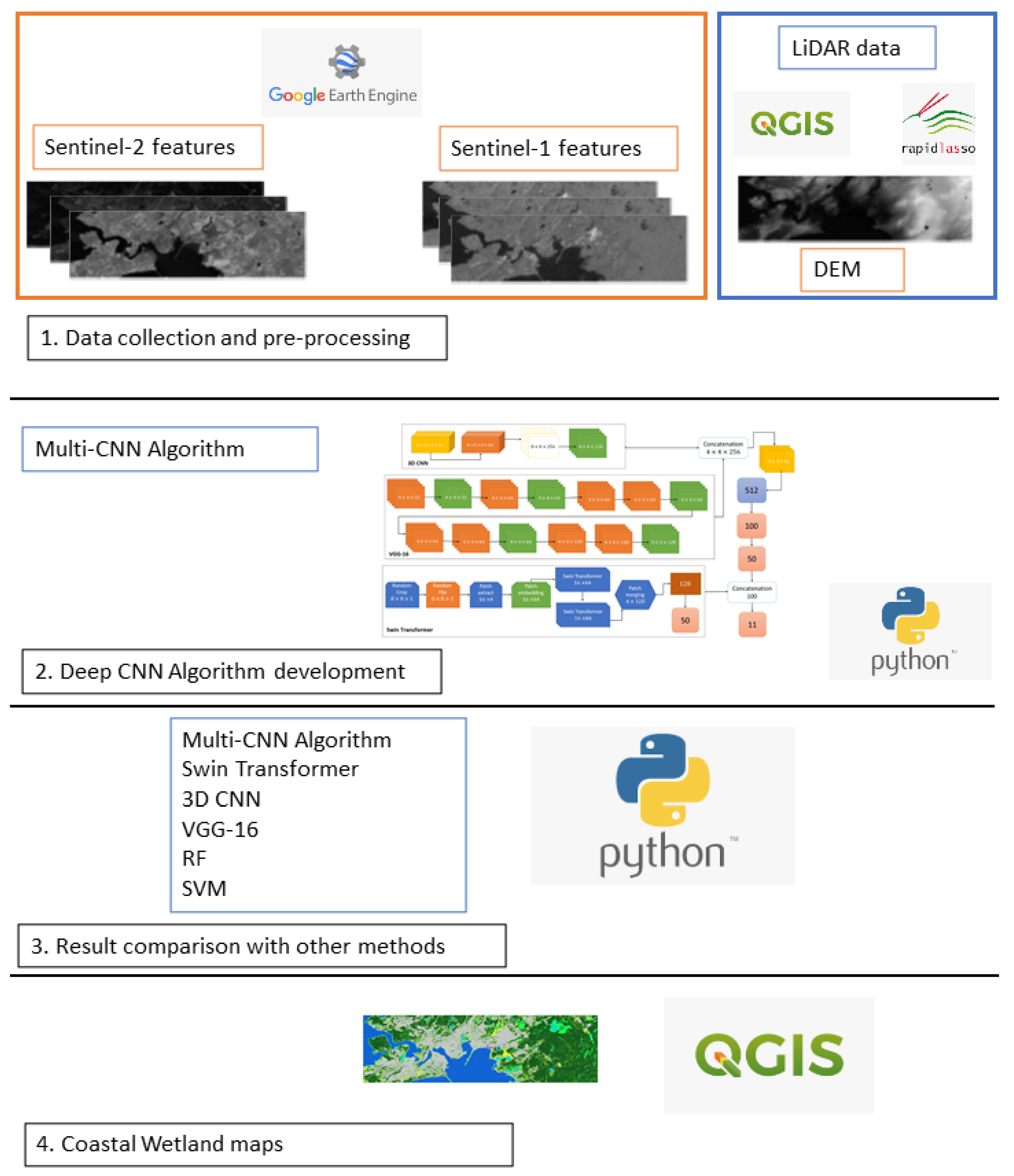
2. Methods
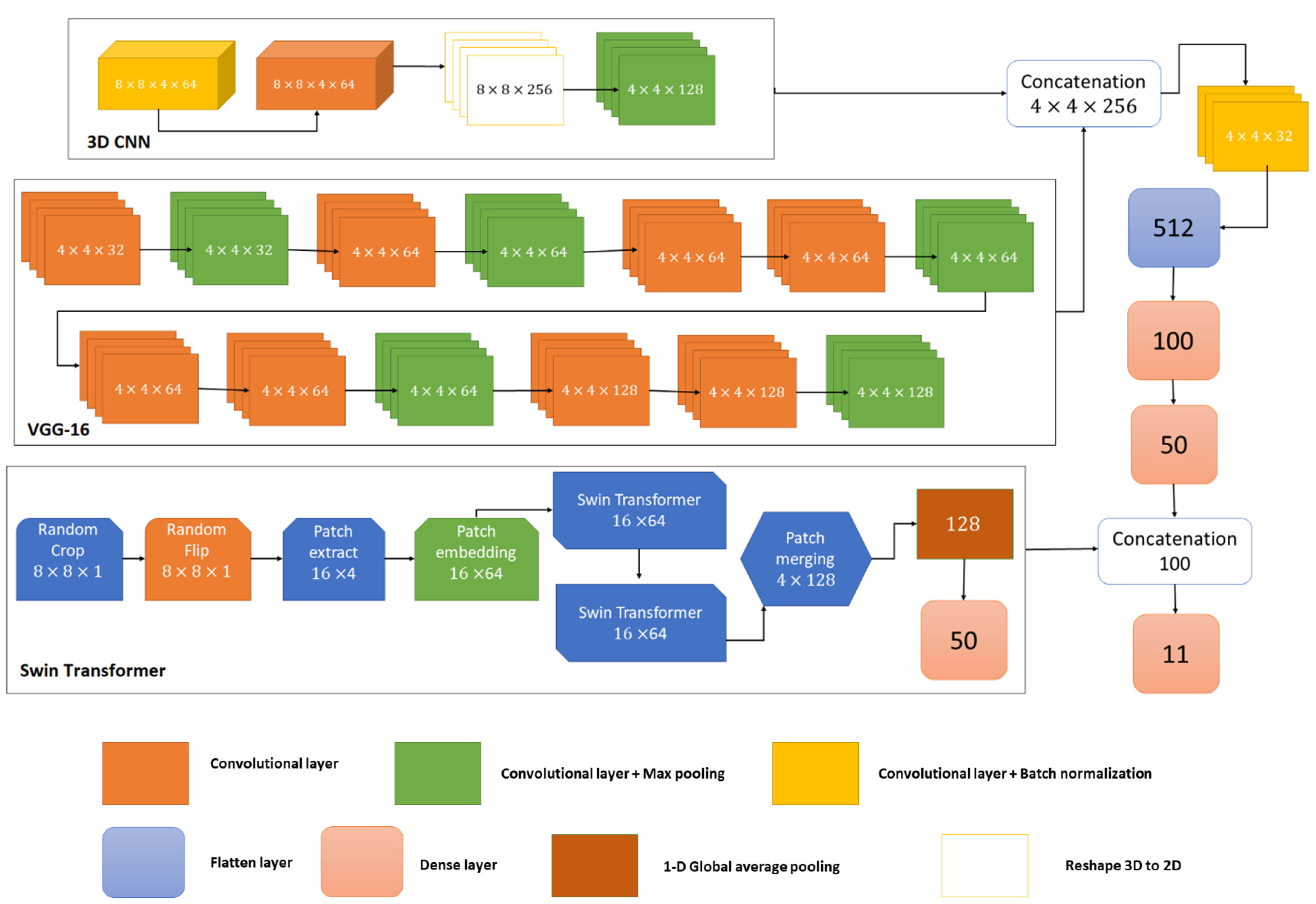
2.1. The Proposed Multi-Model Deep Learning Classifier
2.2. Study Area and Data Collection
2.3. Experimental Setting
2.4. Evaluation Metrics
2.5. Comparison with Other Classifiers
3. Results
3.1. Comparison Results on the Saint John Pilot Site
3.2. Confusion Matrices
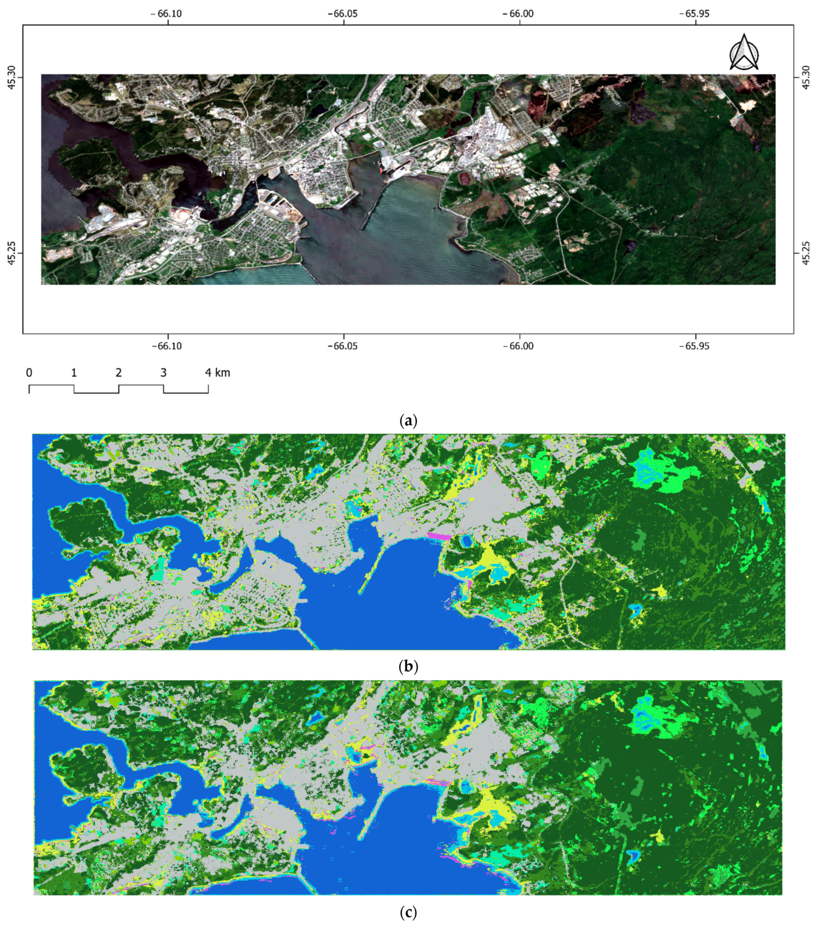
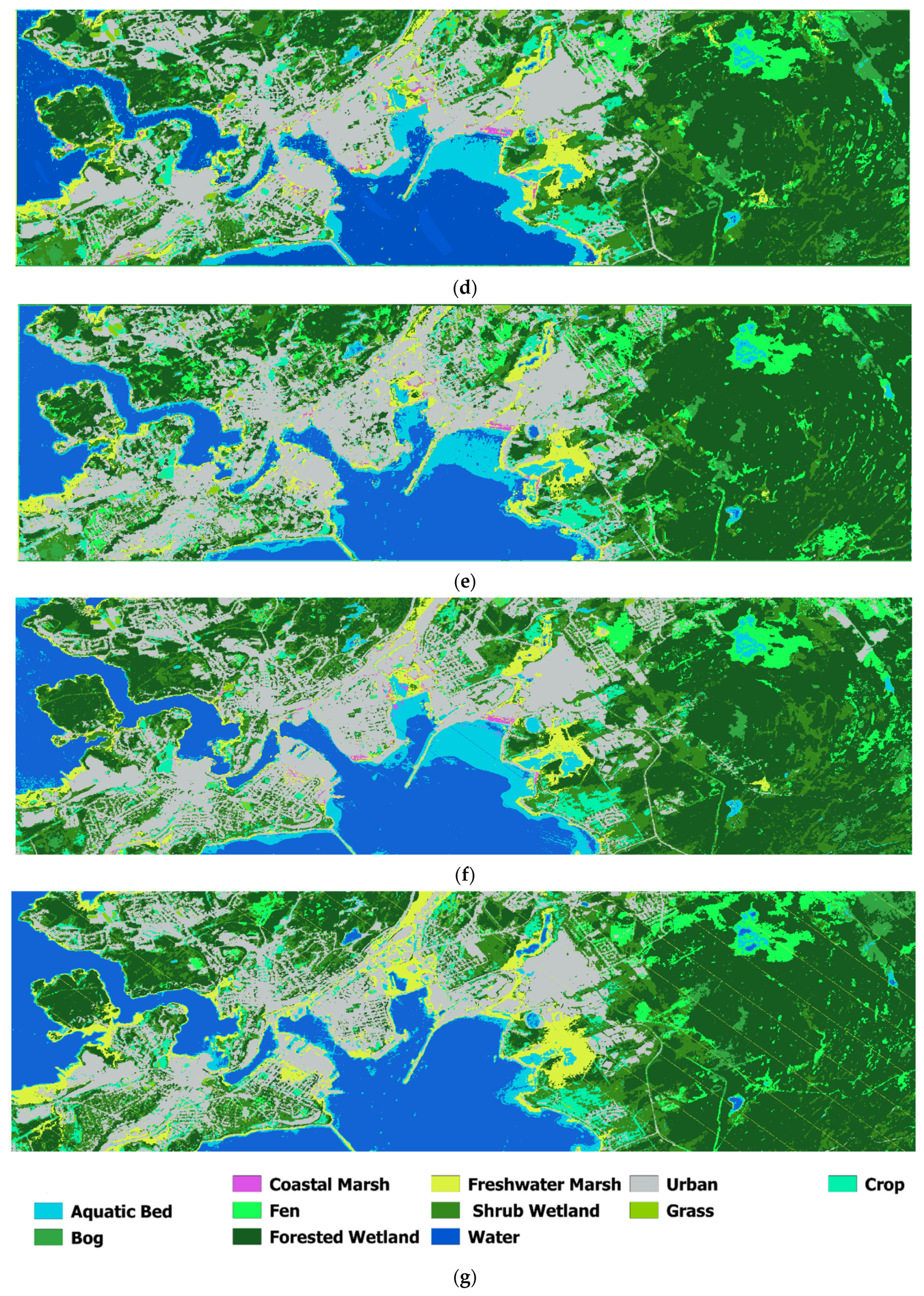
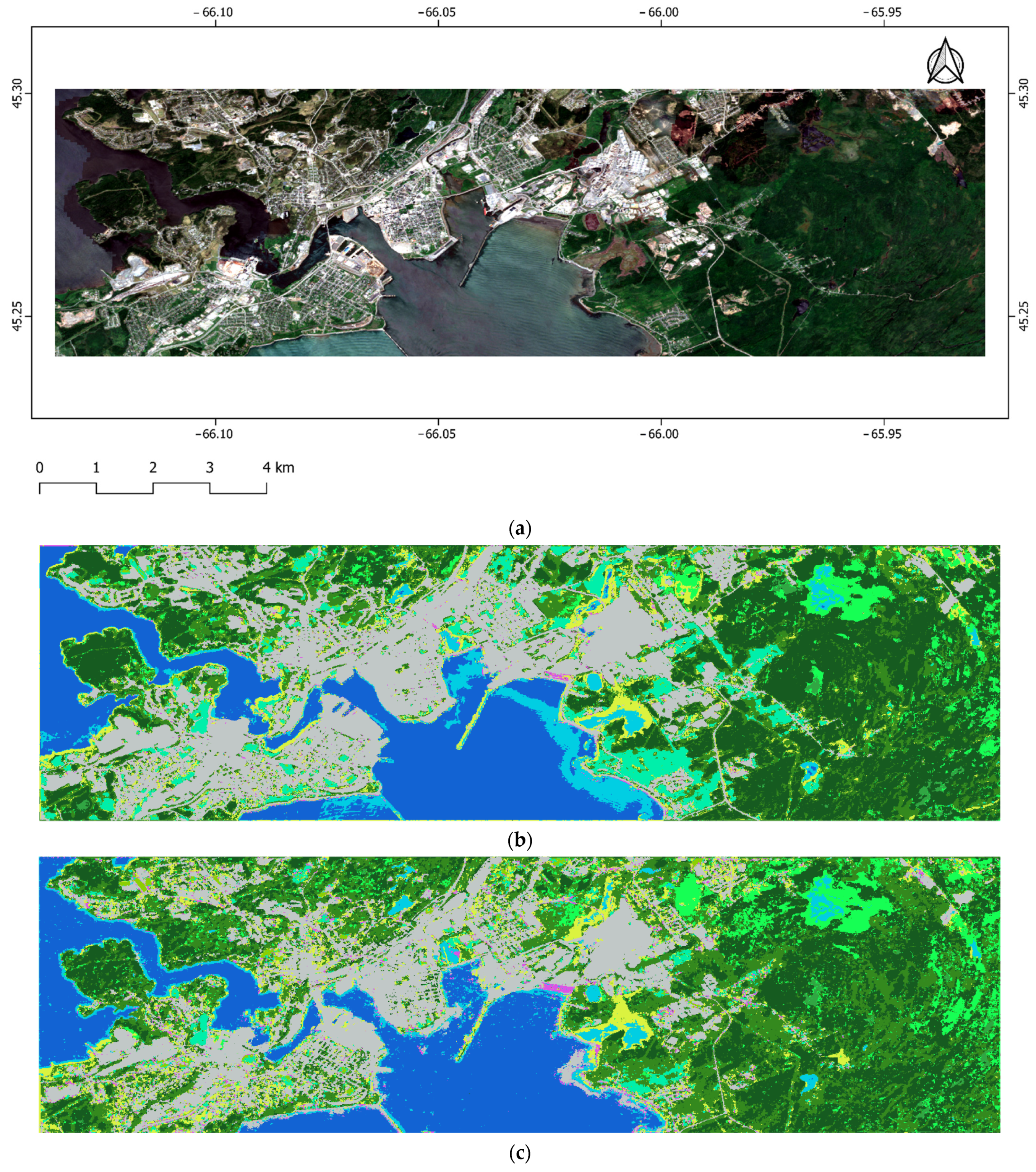
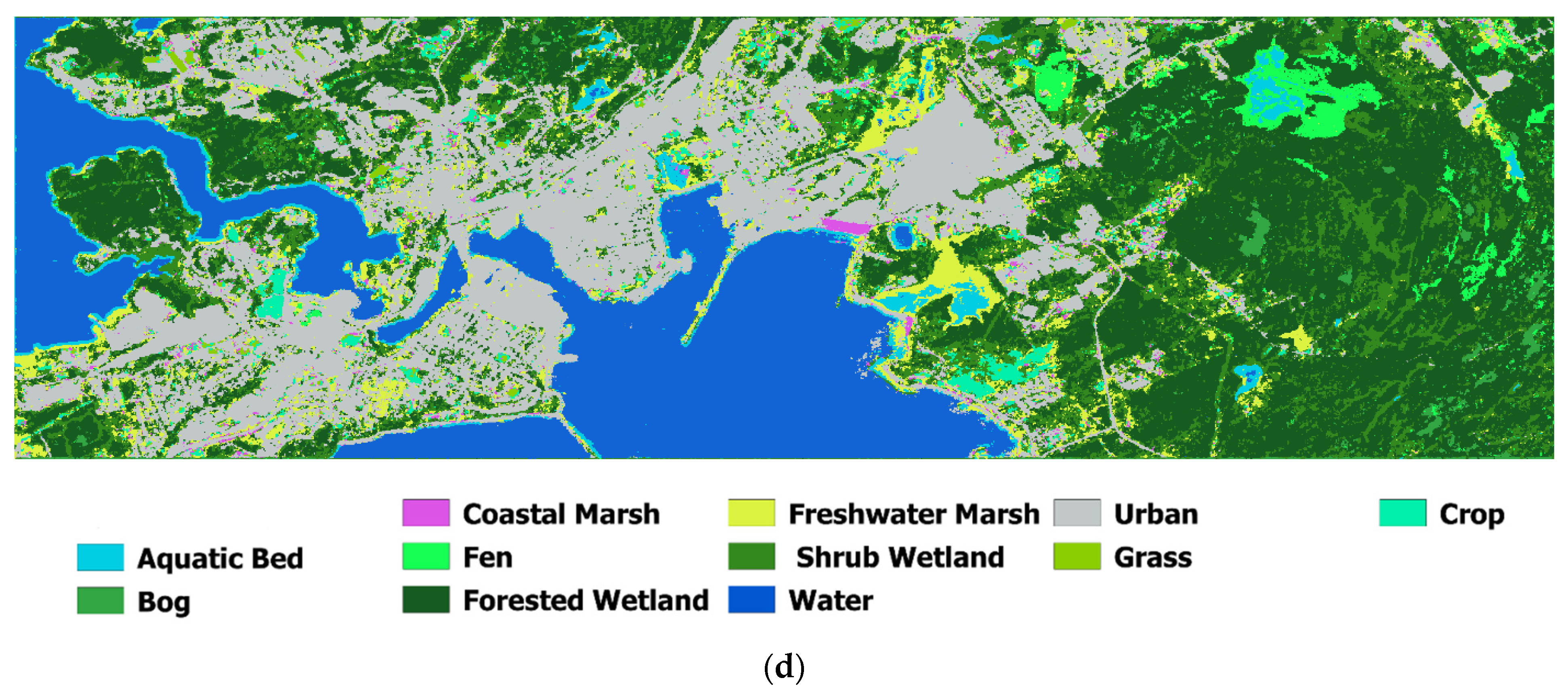
3.3. Classification Maps
3.4. Ablation Study
3.5. Effect of Different Data Sources on Wetland Classification Accuracy
3.6. Effect of Different Spatial Resolutions on Wetland Classification Accuracy
3.7. Computation Cost
4. Discussion
5. Conclusions
Supplementary Materials
Author Contributions
Funding
Institutional Review Board Statement
Informed Consent Statement
Data Availability Statement
Conflicts of Interest
References
- Mahdianpari, M.; Jafarzadeh, H.; Granger, J.E.; Mohammadimanesh, F.; Brisco, B.; Salehi, B.; Homayouni, S.; Weng, Q. A Large-Scale Change Monitoring of Wetlands Using Time Series Landsat Imagery on Google Earth Engine: A Case Study in Newfoundland. GIScience Remote Sens. 2020, 57, 1102–1124. [Google Scholar] [CrossRef]
- Tiner, R.W. Wetland Indicators: A Guide to Wetland Formation, Identification, Delineation, Classification, and Mapping, 2nd ed.; CRC Press: Boca Raton, FL, USA, 2016. [Google Scholar]
- Kaplan, G.; Avdan, U. Monthly Analysis of Wetlands Dynamics Using Remote Sensing Data. ISPRS Int. J. Geo-Inf. 2018, 7, 411. [Google Scholar] [CrossRef] [Green Version]
- Mao, D.; Wang, Z.; Du, B.; Li, L.; Tian, Y.; Jia, M.; Zeng, Y.; Song, K.; Jiang, M.; Wang, Y. National Wetland Mapping in China: A New Product Resulting from Object-Based and Hierarchical Classification of Landsat 8 OLI Images. ISPRS J. Photogramm. Remote Sens. 2020, 164, 11–25. [Google Scholar] [CrossRef]
- Davidson, N.C. The Ramsar Convention on Wetlands. In The Wetland Book I: Structure and Function, Management and Methods; Springer Publishers: Dordrecht, The Netherlands, 2016. [Google Scholar]
- Fariba Mohammadimanesh; Bahram Salehi; Masoud Mahdianpari; Brian Brisco; Eric Gill Full and Simulated Compact Polarimetry SAR Responses to Canadian Wetlands: Separability Analysis and Classification. Remote Sens. 2019, 11, 516. [CrossRef] [Green Version]
- Jamali, A.; Mahdianpari, M.; Brisco, B.; Granger, J.; Mohammadimanesh, F.; Salehi, B. Deep Forest Classifier for Wetland Mapping Using the Combination of Sentinel-1 and Sentinel-2 Data. GIScience Remote Sens. 2021, 58, 1072–1089. [Google Scholar] [CrossRef]
- Mahdianpari, M.; Salehi, B.; Mohammadimanesh, F.; Homayouni, S.; Gill, E. The First Wetland Inventory Map of Newfoundland at a Spatial Resolution of 10 m Using Sentinel-1 and Sentinel-2 Data on the Google Earth Engine Cloud Computing Platform. Remote Sens. 2019, 11, 43. [Google Scholar] [CrossRef] [Green Version]
- Amani, M.; Salehi, B.; Mahdavi, S.; Brisco, B. Spectral Analysis of Wetlands Using Multi-Source Optical Satellite Imagery. ISPRS J. Photogramm. Remote Sens. 2018, 144, 119–136. [Google Scholar] [CrossRef]
- Slagter, B.; Tsendbazar, N.E.; Vollrath, A.; Reiche, J. Mapping Wetland Characteristics Using Temporally Dense Sentinel-1 and Sentinel-2 Data: A Case Study in the St. Lucia Wetlands, South Africa. Int. J. Appl. Earth Obs. Geoinf. 2020, 86, 102009. [Google Scholar] [CrossRef]
- Asselen, S.V.; Verburg, P.H.; Vermaat, J.E.; Janse, J.H. Drivers of Wetland Conversion: A Global Meta-Analysis. PLoS ONE 2013, 8, e81292. [Google Scholar] [CrossRef] [Green Version]
- Mohammadimanesh, F.; Salehi, B.; Mahdianpari, M.; Brisco, B.; Motagh, M. Wetland Water Level Monitoring Using Interferometric Synthetic Aperture Radar (InSAR): A Review. Can. J. Remote Sens. 2018, 44, 247–262. [Google Scholar] [CrossRef]
- Mahdianpari, M.; Salehi, B.; Mohammadimanesh, F.; Brisco, B. An Assessment of Simulated Compact Polarimetric SAR Data for Wetland Classification Using Random Forest Algorithm. Can. J. Remote Sens. 2017, 43, 468–484. [Google Scholar] [CrossRef]
- Mao, D.; Wang, Z.; Wu, J.; Wu, B.; Zeng, Y.; Song, K.; Yi, K.; Luo, L. China’s Wetlands Loss to Urban Expansion. Land Degrad. Dev. 2018, 29, 2644–2657. [Google Scholar] [CrossRef]
- Kirwan, M.L.; Megonigal, J.P. Tidal Wetland Stability in the Face of Human Impacts and Sea-Level Rise. Nature 2013, 504, 53–60. [Google Scholar] [CrossRef] [PubMed]
- Mahdianpari, M.; Granger, J.E.; Mohammadimanesh, F.; Salehi, B.; Brisco, B.; Homayouni, S.; Gill, E.; Huberty, B.; Lang, M. Meta-Analysis of Wetland Classification Using Remote Sensing: A Systematic Review of a 40-Year Trend in North America. Remote Sens. 2020, 12, 1882. [Google Scholar] [CrossRef]
- Connor, R. The United Nations World Water Development Report 2015: Water for a Sustainable World; UNESCO publishing: Paris, France, 2015. [Google Scholar]
- Mahdianpari, M. Advanced Machine Learning Algorithms for Canadian Wetland Mapping Using Polarimetric Synthetic Aperture Radar (PolSAR) and Optical Imagery. Ph.D. Thesis, Memorial University of Newfoundland, St. John’s, NL, Canada, 2019. [Google Scholar]
- Byun, E.; Finkelstein, S.A.; Cowling, S.A.; Badiou, P. Potential Carbon Loss Associated with Post-Settlement Wetland Conversion in Southern Ontario, Canada. Carbon Balance Manag. 2018, 13, 6. [Google Scholar] [CrossRef] [PubMed]
- Breeuwer, A.; Robroek, B.J.M.; Limpens, J.; Heijmans, M.M.P.D.; Schouten, M.G.C.; Berendse, F. Decreased Summer Water Table Depth Affects Peatland Vegetation. Basic Appl. Ecol. 2009, 10, 330–339. [Google Scholar] [CrossRef]
- Edvardsson, J.; Šimanauskienė, R.; Taminskas, J.; Baužienė, I.; Stoffel, M. Increased Tree Establishment in Lithuanian Peat Bogs—Insights from Field and Remotely Sensed Approaches. Sci. Total Environ. 2015, 505, 113–120. [Google Scholar] [CrossRef] [PubMed]
- Boucher, D.; Gauthier, S.; Thiffault, N.; Marchand, W.; Girardin, M.; Urli, M. How Climate Change Might Affect Tree Regeneration Following Fire at Northern Latitudes: A Review. New For. 2020, 51, 543–571. [Google Scholar] [CrossRef] [Green Version]
- Stralberg, D.; Wang, X.; Parisien, M.-A.; Robinne, F.-N.; Sólymos, P.; Mahon, C.L.; Nielsen, S.E.; Bayne, E.M. Wildfire-Mediated Vegetation Change in Boreal Forests of Alberta, Canada. Ecosphere 2018, 9, e02156. [Google Scholar] [CrossRef]
- Zedler, J.B.; Kercher, S. Causes and Consequences of Invasive Plants in Wetlands: Opportunities, Opportunists, and Outcomes. Crit. Rev. Plant Sci. 2004, 23, 431–452. [Google Scholar] [CrossRef]
- Perillo, G.; Wolanski, E.; Cahoon, D.R.; Hopkinson, C.S. Coastal Wetlands: And Integrated Ecosystem Approach; Elsevier: Oxford, UK, 2018. [Google Scholar]
- Hosseiny, B.; Mahdianpari, M.; Brisco, B.; Mohammadimanesh, F.; Salehi, B. WetNet: A Spatial-Temporal Ensemble Deep Learning Model for Wetland Classification Using Sentinel-1 and Sentinel-2. IEEE Trans. Geosci. Remote Sens. 2021, 1–14. [Google Scholar]
- Dawson, T.P.; Jackson, S.T.; House, J.I.; Prentice, I.C.; Mace, G.M. Beyond Predictions: Biodiversity Conservation in a Changing Climate. Science 2011, 332, 53–58. [Google Scholar] [CrossRef] [PubMed] [Green Version]
- Howes, N.C.; FitzGerald, D.M.; Hughes, Z.J.; Georgiou, I.Y.; Kulp, M.A.; Miner, M.D.; Smith, J.M.; Barras, J.A. Hurricane-Induced Failure of Low Salinity Wetlands. Proc. Natl. Acad. Sci. USA 2010, 107, 14014. [Google Scholar] [CrossRef] [PubMed] [Green Version]
- Mitsch, W.J.; Gosselink, J.G. The Value of Wetlands: Importance of Scale and Landscape Setting. Ecol. Econ. 2000, 35, 25–33. [Google Scholar] [CrossRef]
- Zhu, P.; Gong, P. Suitability Mapping of Global Wetland Areas and Validation with Remotely Sensed Data. Sci. China Earth Sci. 2014, 57, 2283–2292. [Google Scholar] [CrossRef]
- Zhu, Q.; Peng, C.; Chen, H.; Fang, X.; Liu, J.; Jiang, H.; Yang, Y.; Yang, G. Estimating Global Natural Wetland Methane Emissions Using Process Modelling: Spatio-Temporal Patterns and Contributions to Atmospheric Methane Fluctuations. Glob. Ecol. Biogeogr. 2015, 24, 959–972. [Google Scholar] [CrossRef]
- Mahdianpari, M.; Brisco, B.; Granger, J.; Mohammadimanesh, F.; Salehi, B.; Homayouni, S.; Bourgeau-Chavez, L. The Third Generation of Pan-Canadian Wetland Map at 10 m Resolution Using Multisource Earth Observation Data on Cloud Computing Platform. IEEE J. Sel. Top. Appl. Earth Obs. Remote Sens. 2021, 14, 8789–8803. [Google Scholar]
- Mahdianpari, M.; Jafarzadeh, H.; Granger, J.E.; Mohammadimanesh, F.; Brisco, B.; Salehi, B.; Homayouni, S.; Weng, Q. Monitoring of 30 Years Wetland Changes in Newfoundland, Canada. In Proceedings of the 2021 IEEE International Geoscience and Remote Sensing Symposium IGARSS, Brussels, Belgium, 11–16 July 2021; pp. 88–91. [Google Scholar]
- Granger, J.E.; Mahdianpari, M.; Puestow, T.; Warren, S.; Mohammadimanesh, F.; Salehi, B.; Brisco, B. Object-Based Random Forest Wetland Mapping in Conne River, Newfoundland, Canada. J. Appl. Remote Sens. 2021, 15, 038506. [Google Scholar] [CrossRef]
- Mahdianpari, M.; Salehi, B.; Mohammadimanesh, F.; Brisco, B.; Homayouni, S.; Gill, E.; DeLancey, E.R.; Bourgeau-Chavez, L. Big Data for a Big Country: The First Generation of Canadian Wetland Inventory Map at a Spatial Resolution of 10-m Using Sentinel-1 and Sentinel-2 Data on the Google Earth Engine Cloud Computing Platform. Can. J. Remote Sens. 2020, 46, 15–33. [Google Scholar] [CrossRef]
- Amani, M.; Brisco, B.; Mahdavi, S.; Ghorbanian, A.; Moghimi, A.; DeLancey, E.R.; Merchant, M.; Jahncke, R.; Fedorchuk, L.; Mui, A.; et al. Evaluation of the Landsat-Based Canadian Wetland Inventory Map Using Multiple Sources: Challenges of Large-Scale Wetland Classification Using Remote Sensing. IEEE J. Sel. Top. Appl. Earth Obs. Remote Sens. 2021, 14, 32–52. [Google Scholar] [CrossRef]
- Mohammadimanesh, F.; Salehi, B.; Mahdianpari, M.; Homayouni, S. Unsupervised Wishart Classfication of Wetlands in Newfoundland, Canada Using Polsar Data Based on Fisher Linear Discriminant Analysis. Int. Arch. Photogramm. Remote Sens. Spat. Inf. Sci. 2016, 41, 305. [Google Scholar] [CrossRef] [Green Version]
- Bennett, K.P. Global Tree Optimization: A Non-Greedy Decision Tree Algorithm. Comput. Sci. Stat. 1994, 26, 156–160. [Google Scholar]
- Belgiu, M.; Drăguţ, L. Random Forest in Remote Sensing: A Review of Applications and Future Directions. ISPRS J. Photogramm. Remote Sens. 2016, 114, 24–31. [Google Scholar] [CrossRef]
- Cortes, C.; Vapnik, V. Support-Vector Networks. Mach. Learn. 1995, 20, 273–297. [Google Scholar] [CrossRef]
- Hamida, A.B.; Benoit, A.; Lambert, P.; Amar, C.B. 3-D Deep Learning Approach for Remote Sensing Image Classification. IEEE Trans. Geosci. Remote Sens. 2018, 56, 4420–4434. [Google Scholar] [CrossRef] [Green Version]
- Algan, G.; Ulusoy, I. Image Classification with Deep Learning in the Presence of Noisy Labels: A Survey. Knowl.-Based Syst. 2021, 215, 106771. [Google Scholar] [CrossRef]
- Hong, D.; Gao, L.; Yokoya, N.; Yao, J.; Chanussot, J.; Du, Q.; Zhang, B. More Diverse Means Better: Multimodal Deep Learning Meets Remote-Sensing Imagery Classification. IEEE Trans. Geosci. Remote Sens. 2021, 59, 4340–4354. [Google Scholar] [CrossRef]
- DeLancey, E.R.; Simms, J.F.; Mahdianpari, M.; Brisco, B.; Mahoney, C.; Kariyeva, J. Comparing Deep Learning and Shallow Learning for Large-Scale Wetland Classification in Alberta, Canada. Remote Sens. 2020, 12, 2. [Google Scholar] [CrossRef] [Green Version]
- Mahdianpari, M.; Salehi, B.; Rezaee, M.; Mohammadimanesh, F.; Zhang, Y. Very Deep Convolutional Neural Networks for Complex Land Cover Mapping Using Multispectral Remote Sensing Imagery. Remote Sens. 2018, 10, 1119. [Google Scholar] [CrossRef] [Green Version]
- Rezaee, M.; Mahdianpari, M.; Zhang, Y.; Salehi, B. Deep Convolutional Neural Network for Complex Wetland Classification Using Optical Remote Sensing Imagery. IEEE J. Sel. Top. Appl. Earth Obs. Remote Sens. 2018, 11, 3030–3039. [Google Scholar] [CrossRef]
- Ghanbari, H.; Mahdianpari, M.; Homayouni, S.; Mohammadimanesh, F. A Meta-Analysis of Convolutional Neural Networks for Remote Sensing Applications. IEEE J. Sel. Top. Appl. Earth Obs. Remote Sens. 2021, 14, 3602–3613. [Google Scholar] [CrossRef]
- Jamali, A.; Mahdianpari, M.; Brisco, B.; Granger, J.; Mohammadimanesh, F.; Salehi, B. Wetland Mapping Using Multi-Spectral Satellite Imagery and Deep Convolutional Neural Networks: A Case Study in Newfoundland and Labrador, Canada. Can. J. Remote Sens. 2021, 47, 243–260. [Google Scholar] [CrossRef]
- Taghizadeh-Mehrjardi, R.; Mahdianpari, M.; Mohammadimanesh, F.; Behrens, T.; Toomanian, N.; Scholten, T.; Schmidt, K. Multi-Task Convolutional Neural Networks Outperformed Random Forest for Mapping Soil Particle Size Fractions in Central Iran. Geoderma 2020, 376, 114552. [Google Scholar] [CrossRef]
- Mahdianpari, M.; Salehi, B.; Mohammadimanesh, F.; Motagh, M. Random Forest Wetland Classification Using ALOS-2 L-Band, RADARSAT-2 C-Band, and TerraSAR-X Imagery. ISPRS J. Photogramm. Remote Sens. 2017, 130, 13–31. [Google Scholar] [CrossRef]
- Mahdianpari, M.; Salehi, B.; Mohammadimanesh, F.; Brisco, B.; Mahdavi, S.; Amani, M.; Granger, J.E. Fisher Linear Discriminant Analysis of Coherency Matrix for Wetland Classification Using PolSAR Imagery. Remote Sens. Environ. 2018, 206, 300–317. [Google Scholar] [CrossRef]
- Jamali, A.; Mahdianpari, M.; Brisco, B.; Granger, J.; Mohammadimanesh, F.; Salehi, B. Comparing Solo Versus Ensemble Convolutional Neural Networks for Wetland Classification Using Multi-Spectral Satellite Imagery. Remote Sens. 2021, 13, 2046. [Google Scholar] [CrossRef]
- Mohammadimanesh, F.; Salehi, B.; Mahdianpari, M.; Gill, E.; Molinier, M. A New Fully Convolutional Neural Network for Semantic Segmentation of Polarimetric SAR Imagery in Complex Land Cover Ecosystem. ISPRS J. Photogramm. Remote Sens. 2019, 151, 223–236. [Google Scholar] [CrossRef]
- Jeppesen, J.H.; Jacobsen, R.H.; Inceoglu, F.; Toftegaard, T.S. A Cloud Detection Algorithm for Satellite Imagery Based on Deep Learning. Remote Sens. Environ. 2019, 229, 247–259. [Google Scholar] [CrossRef]
- Alhichri, H.; Alswayed, A.S.; Bazi, Y.; Ammour, N.; Alajlan, N.A. Classification of Remote Sensing Images Using EfficientNet-B3 CNN Model With Attention. IEEE Access 2021, 9, 14078–14094. [Google Scholar] [CrossRef]
- Kattenborn, T.; Leitloff, J.; Schiefer, F.; Hinz, S. Review on Convolutional Neural Networks (CNN) in Vegetation Remote Sensing. ISPRS J. Photogramm. Remote Sens. 2021, 173, 24–49. [Google Scholar] [CrossRef]
- Khan, M.A.; Akram, T.; Zhang, Y.-D.; Sharif, M. Attributes Based Skin Lesion Detection and Recognition: A Mask RCNN and Transfer Learning-Based Deep Learning Framework. Pattern Recognit. Lett. 2021, 143, 58–66. [Google Scholar] [CrossRef]
- Zhang, C.; Pan, X.; Li, H.; Gardiner, A.; Sargent, I.; Hare, J.; Atkinson, P.M. A Hybrid MLP-CNN Classifier for Very Fine Resolution Remotely Sensed Image Classification. ISPRS J. Photogramm. Remote Sens. 2018, 140, 133–144. [Google Scholar] [CrossRef] [Green Version]
- Cao, J.; Cui, H.; Zhang, Q.; Zhang, Z. Ancient Mural Classification Method Based on Improved AlexNet Network. Stud. Conserv. 2020, 65, 411–423. [Google Scholar] [CrossRef]
- He, K.; Zhang, X.; Ren, S.J.; Sun, J. Deep Residual Learning for Image Recognition. In Proceedings of the IEEE Conference on Computer Vision and Pattern Recognition (CVPR) 2016, Las Vegas, NV, USA, 27–30 June 2016; pp. 770–778. [Google Scholar]
- Huang, G.; Liu, Z.; Van Der Maaten, L.; Weinberger, K.Q. Densely Connected Convolutional Networks. In Proceedings of the IEEE Conference on Computer Vision and Pattern Recognition 2017, Honolulu, HI, USA, 21–26 July 2017; pp. 4700–4708. [Google Scholar]
- Xie, S.; Girshick, R.; Dollár, P.; Tu, Z.; He, K. Aggregated ’Residual Transformations for Deep Neural Networks. In Proceedings of the IEEE Conference on Computer Vision and Pattern Recognition 2017, Honolulu, HI, USA, 21–26 July 2017. [Google Scholar]
- Vaswani, A.; Shazeer, N.; Parmar, N.; Uszkoreit, J.; Jones, L.; Gomez, A.N.; Kaiser, Ł.; Polosukhin, I. Attention Is All You Need. In Proceedings of the Advances in Neural Information Processing Systems, Long Beach, CA, USA, 4–9 December 2017; pp. 5998–6008. [Google Scholar]
- Bazi, Y.; Bashmal, L.; Rahhal, M.M.A.; Dayil, R.A.; Ajlan, N.A. Vision Transformers for Remote Sensing Image Classification. Remote Sens. 2021, 13, 516. [Google Scholar] [CrossRef]
- He, J.; Zhao, L.; Yang, H.; Zhang, M.; Li, W. HSI-BERT: Hyperspectral Image Classification Using the Bidirectional Encoder Representation From Transformers. IEEE Trans. Geosci. Remote Sens. 2020, 58, 165–178. [Google Scholar] [CrossRef]
- Hong, D.; Han, Z.; Yao, J.; Gao, L.; Zhang, B.; Plaza, A.; Chanussot, J. SpectralFormer: Rethinking Hyperspectral Image Classification with Transformers. IEEE Trans. Geosci. Remote Sens. 2021, 1. [Google Scholar] [CrossRef]
- Mohammadimanesh, F.; Salehi, B.; Mahdianpari, M.; Brisco, B.; Motagh, M. Multi-Temporal, Multi-Frequency, and Multi-Polarization Coherence and SAR Backscatter Analysis of Wetlands. ISPRS J. Photogramm. Remote Sens. 2018, 142, 78–93. [Google Scholar] [CrossRef]
- Louis, J.; Debaecker, V.; Pflug, B.; Main-Knorn, M.; Bieniarz, J.; Mueller-Wilm, U.; Cadau, E.; Gascon, F. Sentinel-2 Sen2Cor: L2A Processor for Users. In Living Planet Symposium 2016, SP-740, Proceedings of the ESA Living Planet Symposium 2016, Prague, Czech Republic, 9–13 May 2016; Spacebooks Online: Bavaria, Germany, 2016; pp. 1–8. ISBN 978-92-9221-305-3. ISSN 1609-042X. [Google Scholar]
- Liu, Z.; Lin, Y.; Cao, Y.; Hu, H.; Wei, Y.; Zhang, Z.; Lin, S.; Guo, B. Swin Transformer: Hierarchical Vision Transformer Using Shifted Windows. arXiv 2021, arXiv:2103.14030. [Google Scholar]
- Breiman, L. Random Forests. Mach. Learn. 2001, 54, 5–32. [Google Scholar] [CrossRef] [Green Version]
- Azeez, N.; Yahya, W.; Al-Taie, I.; Basbrain, A.; Clark, A. Regional Agricultural Land Classification Based on Random Forest (RF), Decision Tree, and SVMs Techniques; Springer: Berlin/Heidelberg, Germany, 2020; pp. 73–81. [Google Scholar]
- Collins, L.; McCarthy, G.; Mellor, A.; Newell, G.; Smith, L. Training Data Requirements for Fire Severity Mapping Using Landsat Imagery and Random Forest. Remote Sens. Environ. 2020, 245, 111839. [Google Scholar] [CrossRef]
- Rodriguez-Galiano, V.F.; Ghimire, B.; Rogan, J.; Chica-Olmo, M.; Rigol-Sanchez, J.P. An Assessment of the Effectiveness of a Random Forest Classifier for Land-Cover Classification. ISPRS J. Photogramm. Remote Sens. 2012, 67, 93–104. [Google Scholar] [CrossRef]
- Aldrich, C. Process Variable Importance Analysis by Use of Random Forests in a Shapley Regression Framework. Minerals 2020, 10, 420. [Google Scholar] [CrossRef]
- Collins, L.; Griffioen, P.; Newell, G.; Mellor, A. The Utility of Random Forests for Wildfire Severity Mapping. Remote Sens. Environ. 2018, 216, 374–384. [Google Scholar] [CrossRef]
- Gibson, R.; Danaher, T.; Hehir, W.; Collins, L. A Remote Sensing Approach to Mapping Fire Severity in South-Eastern Australia Using Sentinel 2 and Random Forest. Remote Sens. Environ. 2020, 240, 111702. [Google Scholar] [CrossRef]
- Sheykhmousa, M.; Mahdianpari, M.; Ghanbari, H.; Mohammadimanesh, F.; Ghamisi, P.; Homayouni, S. Support Vector Machine Versus Random Forest for Remote Sensing Image Classification: A Meta-Analysis and Systematic Review. IEEE J. Sel. Top. Appl. Earth Obs. Remote Sens. 2020, 13, 6308–6325. [Google Scholar] [CrossRef]
- Razaque, A.; Ben Haj Frej, M.; Almi’ani, M.; Alotaibi, M.; Alotaibi, B. Improved Support Vector Machine Enabled Radial Basis Function and Linear Variants for Remote Sensing Image Classification. Sensors 2021, 21, 4431. [Google Scholar] [CrossRef] [PubMed]
- Liang, J.; Deng, Y.; Zeng, D. A Deep Neural Network Combined CNN and GCN for Remote Sensing Scene Classification. IEEE J. Sel. Top. Appl. Earth Obs. Remote Sens. 2020, 13, 4325–4338. [Google Scholar] [CrossRef]
- Sit, M.; Demiray, B.Z.; Xiang, Z.; Ewing, G.J.; Sermet, Y.; Demir, I. A Comprehensive Review of Deep Learning Applications in Hydrology and Water Resources. Water Sci. Technol. 2020, 82, 2635–2670. [Google Scholar] [CrossRef] [PubMed]
- Ma, L.; Liu, Y.; Zhang, X.; Ye, Y.; Yin, G.; Johnson, B.A. Deep Learning in Remote Sensing Applications: A Meta-Analysis and Review. ISPRS J. Photogramm. Remote Sens. 2019, 152, 166–177. [Google Scholar] [CrossRef]
- Bera, S.; Shrivastava, V.K. Analysis of Various Optimizers on Deep Convolutional Neural Network Model in the Application of Hyperspectral Remote Sensing Image Classification. Int. J. Remote Sens. 2020, 41, 2664–2683. [Google Scholar] [CrossRef]
- Simonyan, K.; Zisserman, A. Very Deep Convolutional Networks for Large-Scale Image Recognition. In Proceedings of the International Conference on Learning Representations, Banff, Canada, 14–16 April 2014. [Google Scholar]
- Srivastava, S.; Kumar, P.; Chaudhry, V.; Singh, A. Detection of Ovarian Cyst in Ultrasound Images Using Fine-Tuned VGG-16 Deep Learning Network. SN Comput. Sci. 2020, 1, 81. [Google Scholar] [CrossRef] [Green Version]
- Quinlan, J.R. C4.5: Programs for Machine Learning; Morgan Kaufmann: San Mateo, CA, USA, 1993. [Google Scholar]
- Amani, M.; Mahdavi, S.; Berard, O. Supervised Wetland Classification Using High Spatial Resolution Optical, SAR, and LiDAR Imagery. J. Appl. Remote Sens. 2020, 14, 024502. [Google Scholar] [CrossRef]
- Jamali, A.; Mahdianpari, M.; Mohammadimanesh, F.; Brisco, B.; Salehi, B. A Synergic Use of Sentinel-1 and Sentinel-2 Imagery for Complex Wetland Classification Using Generative Adversarial Network (GAN) Scheme. Water 2021, 13, 3601. [Google Scholar] [CrossRef]
- LaRocque, A.; Phiri, C.; Leblon, B.; Pirotti, F.; Connor, K.; Hanson, A. Wetland Mapping with Landsat 8 OLI, Sentinel-1, ALOS-1 PALSAR, and LiDAR Data in Southern New Brunswick, Canada. Remote Sens. 2020, 12, 2095. [Google Scholar] [CrossRef]
- Mohammadi, A.; Karimzadeh, S.; Jalal, S.J.; Kamran, K.V.; Shahabi, H.; Homayouni, S.; Al-Ansari, N. A Multi-Sensor Comparative Analysis on the Suitability of Generated DEM from Sentinel-1 SAR Interferometry Using Statistical and Hydrological Models. Sensors 2020, 20, 7214. [Google Scholar] [CrossRef] [PubMed]
- Devaraj, S.; Yarrakula, K. Evaluation of Sentinel 1–Derived and Open-Access Digital Elevation Model Products in Mountainous Areas of Western Ghats, India. Arab. J. Geosci. 2020, 13, 1103. [Google Scholar] [CrossRef]


| Class | Training (Pixels) | Test (Pixels) |
|---|---|---|
| Aquatic bed | 4633 | 4633 |
| Bog | 2737 | 2737 |
| Coastal marsh | 607 | 608 |
| Fen | 11,306 | 11,305 |
| Forested wetland | 23,212 | 23,212 |
| Freshwater marsh | 5233 | 5232 |
| Shrub wetland | 11,285 | 11,285 |
| Water | 5058 | 5059 |
| Urban | 8129 | 8129 |
| Grass | 718 | 717 |
| Crop | 1409 | 1410 |
| Data | Normalized Backscattering Coefficients/Spectral Bands | Spectral Indices |
|---|---|---|
| Sentinel-1 | , , , | |
| Sentinel-2 | B2, B3, B4, B5, B6, B7, B8, B8A, B11, B12 | |
| Model | AB | BO | CM | FE | FW | FM | SB | W | U | G | C | AA (%) | OA (%) | K (%) |
|---|---|---|---|---|---|---|---|---|---|---|---|---|---|---|
| Multi-model | 92.68 | 92.30 | 90.65 | |||||||||||
| Precision | 0.92 | 0.89 | 0.96 | 0.97 | 0.89 | 0.92 | 0.89 | 0.99 | 0.98 | 0.99 | 0.99 | |||
| Recall | 0.91 | 0.90 | 0.89 | 0.81 | 0.97 | 0.94 | 0.86 | 1 | 1 | 0.97 | 0.96 | |||
| F-1 score | 0.91 | 0.89 | 0.93 | 0.88 | 0.93 | 0.93 | 0.87 | 1 | 99 | 0.98 | 0.98 | |||
| Swin Transformer | 78.75 | 79.79 | 75.36 | |||||||||||
| Precision | 0.85 | 0.69 | 0.82 | 0.75 | 0.76 | 0.78 | 0.75 | 0.94 | 0.94 | 0.93 | 0.90 | |||
| Recall | 0.78 | 0.67 | 0.58 | 0.68 | 0.89 | 0.90 | 0.52 | 0.99 | 0.95 | 0.79 | 0.91 | |||
| F-1 score | 0.81 | 0.68 | 0.68 | 0.72 | 0.82 | 0.83 | 0.62 | 0.97 | 0.94 | 0.85 | 0.91 | |||
| 3DCNN | 83.76 | 85.38 | 82.13 | |||||||||||
| Precision | 0.88 | 0.79 | 0.95 | 0.79 | 0.80 | 0.90 | 0.87 | 0.99 | 0.99 | 0.81 | 0.97 | |||
| Recall | 0.86 | 0.67 | 0.64 | 0.78 | 0.95 | 0.89 | 0.61 | 0.99 | 0.99 | 0.96 | 0.88 | |||
| F-1 score | 0.87 | 0.73 | 0.77 | 0.78 | 0.87 | 0.90 | 0.72 | 0.99 | 0.99 | 0.88 | 0.92 | |||
| VGG-16 | 75.37 | 81.13 | 76.76 | |||||||||||
| Precision | 0.90 | 0.85 | 0.84 | 0.83 | 0.73 | 0.80 | 0.79 | 0.98 | 0.94 | 0.88 | 0.90 | |||
| Recall | 0.82 | 0.52 | 0.35 | 0.68 | 0.95 | 0.89 | 0.54 | 1 | 0.94 | 0.74 | 0.88 | |||
| F-1 score | 0.85 | 0.64 | 0.49 | 0.75 | 0.83 | 0.84 | 0.64 | 0.99 | 0.94 | 0.80 | 0.89 | |||
| RF | 89.32 | 91.54 | 89.74 | |||||||||||
| Precision | 0.93 | 0.97 | 0.89 | 0.92 | 0.88 | 0.91 | 0.88 | 1 | 0.97 | 0.98 | 0.94 | |||
| Recall | 0.91 | 0.84 | 0.66 | 0.88 | 0.94 | 0.93 | 0.83 | 1 | 0.99 | 0.89 | 0.96 | |||
| F-1 score | 0.92 | 0.90 | 0.76 | 0.90 | 0.91 | 0.92 | 0.85 | 1 | 0.98 | 0.93 | 0.95 | |||
| SVM | 59.33 | 69.47 | 62.18 | |||||||||||
| Precision | 0.74 | 0.71 | 0 | 0.64 | 0.66 | 0.56 | 0.61 | 0.86 | 0.94 | 0.81 | 0.77 | |||
| Recall | 0.55 | 0.27 | 0 | 0.58 | 0.91 | 0.82 | 0.24 | 0.99 | 0.89 | 0.55 | 0.73 | |||
| F-1 score | 0.63 | 0.39 | 0 | 0.60 | 0.77 | 0.66 | 0.34 | 0.92 | 0.91 | 0.65 | 0.75 |
| Model | AB | BO | CM | FE | FW | FM | SB | W | U | G | C | AA (%) | OA (%) | K (%) |
|---|---|---|---|---|---|---|---|---|---|---|---|---|---|---|
| VGG-16 | 73.93 | 79.75 | 75.46 | |||||||||||
| Precision | 0.82 | 0.78 | 0.81 | 0.70 | 0.83 | 0.75 | 0.65 | 0.99 | 0.95 | 0.92 | 0.70 | |||
| Recall | 0.82 | 0.40 | 0.44 | 0.74 | 0.86 | 0.77 | 0.61 | 1 | 1 | 0.51 | 0.99 | |||
| F-1 score | 0.82 | 0.53 | 0.57 | 0.72 | 0.84 | 0.76 | 0.63 | 1 | 0.98 | 0.66 | 0.82 | |||
| VGG-16 + 3DCNN | 91.14 | 89.37 | 87.29 | |||||||||||
| Precision | 0.92 | 0.99 | 0.89 | 0.80 | 0.97 | 0.93 | 0.74 | 1 | 1 | 0.96 | 0.97 | |||
| Recall | 0.92 | 0.69 | 0.88 | 0.95 | 0.80 | 0.92 | 0.94 | 1 | 0.97 | 0.99 | 0.97 | |||
| F-1 score | 0.92 | 0.81 | 0.89 | 0.87 | 0.88 | 0.93 | 0.83 | 1 | 0.98 | 0.98 | 0.97 | |||
| Multi-model | 92.68 | 92.30 | 90.65 | |||||||||||
| Precision | 0.92 | 0.89 | 0.96 | 0.97 | 0.89 | 0.92 | 0.89 | 0.99 | 0.98 | 0.99 | 0.99 | |||
| Recall | 0.91 | 0.90 | 0.89 | 0.81 | 0.97 | 0.94 | 0.86 | 1 | 1 | 0.97 | 0.96 | |||
| F-1 score | 0.91 | 0.89 | 0.93 | 0.88 | 0.93 | 0.93 | 0.87 | 1 | 99 | 0.98 | 0.98 |
| Model | AB | BO | CM | FE | FW | FM | SB | W | U | G | C | AA (%) | OA (%) | K (%) |
|---|---|---|---|---|---|---|---|---|---|---|---|---|---|---|
| RF-S2 | 83.14 | 87.28 | 84.54 | |||||||||||
| Precision | 0.87 | 0.92 | 0.85 | 0.86 | 0.86 | 0.84 | 0.81 | 1 | 0.95 | 0.95 | 0.90 | |||
| Recall | 0.86 | 0.70 | 0.50 | 0.83 | 0.93 | 0.78 | 0.76 | 1 | 0.98 | 0.85 | 0.94 | |||
| F-1 score | 0.87 | 0.80 | 0.63 | 0.84 | 0.89 | 0.81 | 0.78 | 1 | 0.97 | 0.90 | 0.92 | |||
| RF-S1S2 | 83.84 | 87.72 | 85.05 | |||||||||||
| Precision | 0.89 | 0.95 | 0.92 | 0.85 | 0.85 | 0.88 | 0.81 | 1 | 0.96 | 0.97 | 0.91 | |||
| Recall | 0.89 | 0.65 | 0.54 | 0.83 | 0.94 | 0.80 | 0.76 | 1 | 0.99 | 0.88 | 0.96 | |||
| F-1 score | 0.89 | 0.77 | 0.68 | 0.84 | 0.89 | 0.84 | 0.79 | 1 | 0.97 | 0.92 | 0.93 | |||
| RF-S1S2DEM | 89.32 | 91.54 | 89.74 | |||||||||||
| Precision | 0.93 | 0.97 | 0.89 | 0.92 | 0.88 | 0.91 | 0.88 | 1 | 0.97 | 0.98 | 0.94 | |||
| Recall | 0.91 | 0.84 | 0.66 | 0.88 | 0.94 | 0.93 | 0.83 | 1 | 0.99 | 0.89 | 0.96 | |||
| F-1 score | 0.92 | 0.90 | 0.76 | 0.90 | 0.91 | 0.92 | 0.85 | 1 | 0.98 | 0.93 | 0.95 |
| Model | AB | BO | CM | FE | FW | FM | SB | W | U | G | C | AA (%) | OA (%) | K (%) |
|---|---|---|---|---|---|---|---|---|---|---|---|---|---|---|
| Multi-model-10 | 92.68 | 92.30 | 90.65 | |||||||||||
| Precision | 0.92 | 0.89 | 0.96 | 0.97 | 0.89 | 0.92 | 0.89 | 0.99 | 0.98 | 0.99 | 0.99 | |||
| Recall | 0.91 | 0.90 | 0.89 | 0.81 | 0.97 | 0.94 | 0.86 | 1 | 1 | 0.97 | 0.96 | |||
| F-1 score | 0.91 | 0.89 | 0.93 | 0.88 | 0.93 | 0.93 | 0.87 | 1 | 99 | 0.98 | 0.98 | |||
| Multi-model-30 | 11 | 7 | 9 | 12 | 5 | 19 | 11 | 84.97 | 84.62 | 81.39 | ||||
| Precision | 0.79 | 0.89 | 0.94 | 0.92 | 0.83 | 0.60 | 0.90 | 0.99 | 0.96 | 0.96 | 0.70 | |||
| Recall | 0.81 | 0.76 | 0.76 | 0.65 | 0.94 | 0.94 | 0.65 | 1 | 0.99 | 0.86 | 0.97 | |||
| F-1 score | 0.80 | 0.82 | 0.84 | 0.76 | 0.88 | 0.74 | 0.76 | 0.99 | 0.97 | 0.91 | 0.82 |
Publisher’s Note: MDPI stays neutral with regard to jurisdictional claims in published maps and institutional affiliations. |
© 2022 by the authors. Licensee MDPI, Basel, Switzerland. This article is an open access article distributed under the terms and conditions of the Creative Commons Attribution (CC BY) license (https://creativecommons.org/licenses/by/4.0/).
Share and Cite
Jamali, A.; Mahdianpari, M. Swin Transformer and Deep Convolutional Neural Networks for Coastal Wetland Classification Using Sentinel-1, Sentinel-2, and LiDAR Data. Remote Sens. 2022, 14, 359. https://doi.org/10.3390/rs14020359
Jamali A, Mahdianpari M. Swin Transformer and Deep Convolutional Neural Networks for Coastal Wetland Classification Using Sentinel-1, Sentinel-2, and LiDAR Data. Remote Sensing. 2022; 14(2):359. https://doi.org/10.3390/rs14020359
Chicago/Turabian StyleJamali, Ali, and Masoud Mahdianpari. 2022. "Swin Transformer and Deep Convolutional Neural Networks for Coastal Wetland Classification Using Sentinel-1, Sentinel-2, and LiDAR Data" Remote Sensing 14, no. 2: 359. https://doi.org/10.3390/rs14020359
APA StyleJamali, A., & Mahdianpari, M. (2022). Swin Transformer and Deep Convolutional Neural Networks for Coastal Wetland Classification Using Sentinel-1, Sentinel-2, and LiDAR Data. Remote Sensing, 14(2), 359. https://doi.org/10.3390/rs14020359