Mitigating Atmospheric Effects in InSAR Stacking Based on Ensemble Forecasting with a Numerical Weather Prediction Model

Abstract

The interferometric synthetic aperture radar (InSAR) technique is widely utilized to measure ground-surface displacement. One of the main limitations of the measurements is the atmospheric phase delay effects. For satellites with shorter wavelengths, the atmospheric delay mainly consists of the tropospheric delay influenced by temperature, pressure, and water vapor. Tropospheric delay can be calculated using numerical weather prediction (NWP) model at the same moment as synthetic aperture radar (SAR) acquisition. Scientific researchers mainly use ensemble forecasting to produce better forecasts and analyze the uncertainties caused by physic parameterizations. In this study, we simulated the relevant meteorological parameters using the ensemble scheme of the stochastic physic perturbation tendency (SPPT) based on the weather research forecasting (WRF) model, which is one of the most broadly used NWP models. We selected an area in Foshan, Guangdong Province, in the southeast of China, and calculated the corresponding atmospheric delay. InSAR images were computed through data from the Sentinel-1A satellite and mitigated by the ensemble mean of the WRF-SPPT results. The WRF-SPPT method improves the mitigating effect more than WRF simulation without ensemble forecasting. The atmospherically corrected InSAR phases were used in the stacking process to estimate the linear deformation rate in the experimental area. The root mean square errors (RMSE) of the deformation rate without correction, with WRF-only correction, and with WRF-SPPT correction were calculated, indicating that ensemble forecasting can significantly reduce the atmospheric delay in stacking. In addition, the ensemble forecasting based on a combination of initial uncertainties and stochastic physic perturbation tendencies showed better correction performance compared with the ensemble forecasting generated by a set of perturbed initial conditions without considering the model’s uncertainties.

1. Introduction

Interferometric synthetic aperture radar (InSAR) is a modern technique that has been utilized to identify displacement [1,2], volcano activity, etc. [3,4]. However, measurements from InSAR are usually influenced by the phase delay in the atmosphere, which could reduce the accuracy of subsidence information. A change in humidity of around 20 percent can exist in some extreme cases. Such a change can severely influence the accuracy of the InSAR technique and can even result in errors of up to 10 cm when measuring displacement [5]. Therefore, when we require a high level of accuracy under some specific circumstances, it is necessary to mitigate the undesirable atmospheric effects.

Atmospheric delay consists of two major components: the ionospheric effect and the tropospheric effect [6]. The ionospheric delay is dispersive [7], meaning that it is inversely proportional to the signal frequency. Longer wavelength signals, especially P-band and L-band signals, are impacted severely by the ionosphere. Many mature methods are used in InSAR processing to remove the ionospheric influence. The most widely used approach is the split-spectrum method. After splitting the range spectrum, the original interferometry image can be divided into two sub-images with different frequencies. Then, the ionospheric delay can be calculated.

For satellites with shorter wavelengths (e.g., Envisat and Sentinel-1A), the ionospheric impact is often neglected or estimated by external data [8]. The tropospheric effect has been more widely taken into account for accurate displacement monitoring. Tropospheric delay [9] is influenced by variations in temperature, pressure, and water vapor over time and in space. Many studies have focused on different methodologies to mitigate tropospheric delay. One method relies on the correlation between the delay and topographic elevation [10,11]. Unfortunately, if the phase of subsidence is similar to the atmospheric delay, the deformation and atmospheric contribution become more indistinguishable. Another approach [12,13] uses auxiliary datasets such as from the Medium-Resolution Imaging Spectrometer (MERIS) [14] and from the Moderate-Resolution Imaging Spectroradiometer (MODIS) [15]. However, this method is limited in several aspects: both MERIS and MODIS data have limitations in spatial coverage on cloudy days; the individual MODIS sensors have a large temporal gap when obtaining observational data, which means poor time resolution; and MERIS stopped working in 2012. By integrating the water vapor content from the sensor to the ground, global positioning system (GPS) data have also been successfully taken advantage of to mitigate atmospheric delay. However, GPS has a sparse spatial distribution, and this method needs spatial interpolation.

Recent studies have focused on the weather-based methods [12] which are more feasible and have more potential. These methods rely on weather parameters (e.g., pressure, temperature, and relative humidity) derived from meteorological reanalysis datasets, such as ERA-Interim [16,17] and ERA5 [18] obtained from the European Center for Medium Range Weather Forecasts (ECMWF); or the forecasting products of numerical weather prediction (NWP) models, such as the Fifth-Generation Penn State/National Center for Atmospheric Research (NCAR) Mesoscale Model (MM5) [13], the mesoscale analysis model [19,20] from the Japanese Meteorologic Agency (MANAL), and the weather research and forecasting (WRF) model [21,22,23,24]. NWP models can integrate the water vapor content at the same moment as synthetic aperture radar (SAR) acquisitions, regardless of the presence of clouds.

However, the accuracy of the prediction can be influenced by the input data and the model itself [25]. The ensemble technique is considered a promising approach for obtaining better predictions. Previous studies have generated ensembles through variations in the initial states, which were later found to be insufficient for representing forecast uncertainties. In addition, the model uncertainty has been taken into consideration and efforts have been made to reasonably reduce the model errors [26,27] in recent years. Some researchers use a multi-model ensemble method and take the overall uncertainty from different models into consideration, or use a multi-physics scheme in a single model. Other ensemble approaches have focused on stochastic physics parameterization, introducing perturbations into the equations of the NWP models. Some researchers have made efforts to take advantage of the stochastic total tendency perturbation (STTP) scheme, which represents the uncertainty concerning both the physics and the dynamics in a single model. Some studies have utilized the scheme of stochastic physic perturbation tendency (SPPT), where the uncertainty is related to the total model physical process [28]. In addition, another approach has been used to present the uncertainty in the stochastic kinetic energy backscatter (SKEB) scheme [29]. Random patterns are added to the forecast model to perturb the wind component and potential temperature. By considering the different sources of uncertainties and errors, the ensemble mean could outperform deterministic forecasts [30].

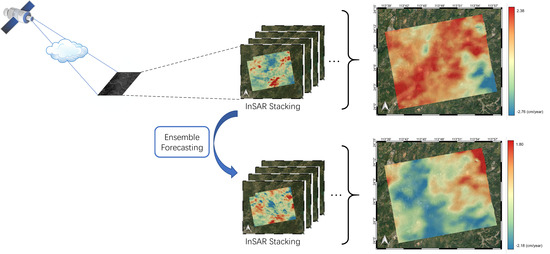
In this study, we took advantage of the ensemble forecasting method to enhance the performance of atmospheric mitigation for the InSAR technique. The experimental area is located in Foshan, Guangdong Province, in the southeast of China. InSAR images were computed through data from the Sentinel-1A satellite. We chose the WRF model as the base model for integration. The SPPT scheme was added to the WRF model to perturb the total parameterization tendency of the physics packages for the wind, potential temperature, and relative humidity. The water vapor content was then integrated at the SAR acquisition time to correct the respective InSAR images. Finally, the atmospherically corrected phases were employed in InSAR stacking to obtain the linear deformation rate of this area.

This manuscript is organized as follows: the background is introduced in Section 1; Section 2 describes the experimental dataset and the WRF-SPPT ensemble method; Section 3 shows the mitigation results achieved in the process of stacking; Section 4 analyzes and discusses the corrected results; and the conclusions are presented in Section 5. Finally, the Appendix A shows a comparison between different WRF-related methods considering the uncertainties in the analysis and forecasting products used in the initial state.

2. Materials and Methods

2.1. Experimental Dataset

In this experiment, we used the area of Foshan, Guangdong Province, in the southeast of China, which is outlined by a red rectangle in Figure 1.

Figure 1. The experimental area in Foshan.

We used 13 SAR images from the Sentinel-1A satellite for stacking. The data are given in IW beam mode (path 11, frame 71). Additionally, the flight direction was ascending. The acquisition dates are listed in Table 1.

Table 1. The acquisition dates of 13 synthetic aperture radar (SAR) images for stacking.

13 December 2017	25 December 2017	8 December 2018
20 December 2018	13 January 2019	25 January 2019
28 October 2019	9 November 2019	3 December 2019
15 December 2019	27 December 2019	20 January 2020
1 February 2020

2.2. Atmospheric Phase Delay in InSAR

2.2.1. InSAR Analysis

The phase observed by InSAR can be decomposed into different parts as follows:

$$\mathsf{\Delta }{\phi }_{int}=\mathsf{\Delta }{\phi }_{topo}+\mathsf{\Delta }{\phi }_{orbit}+\mathsf{\Delta }{\phi }_{defo}+\mathsf{\Delta }{\phi }_{atm}+\mathsf{\Delta }{\phi }_{noise}$$

(1)

where $\mathsf{\Delta }{\phi }_{int}$ represents the interferometric phase between master and slave SAR images. $\mathsf{\Delta }{\phi }_{topo}$, $\mathsf{\Delta }{\phi }_{orbit}$, $\mathsf{\Delta }{\phi }_{defo}$, $\mathsf{\Delta }{\phi }_{atm}$, and $\mathsf{\Delta }{\phi }_{noise}$ are the topographic phase, the orbit phase derived from the curvature of the Earth, the phase of surface subsidence in the radar line-of-sight (LOS) direction, the atmospheric delay phase, and the phase noise resulting from decorrelation of the InSAR signals, respectively. The goal of the InSAR technique is to obtain the surface subsidence. Therefore, the other components in Equation (1) should be removed. $\mathsf{\Delta }{\phi }_{topo}$ can be removed by simulating a phase from a a digital elevation model (DEM) and by subtracting it. $\mathsf{\Delta }{\phi }_{orbit}$ can be eliminated by utilizing the precise orbit data. $\mathsf{\Delta }{\phi }_{noise}$ can be removed by filtering. Next, we discuss the phase contribution of the atmosphere $\mathsf{\Delta }{\phi }_{atm}$ in detail in this manuscript.

2.2.2. Atmospheric Phase Delay with Integration Method

The refractivity of the atmosphere [12,13,16] can be divided into different sections as follows:

$$N_{all}=k_1\frac{P_0}{T}+\left(k_2\frac{e}{T}+k_3\frac{e}{T^2}\right)-\left(4.03\times {10}^7\frac{n_e}{f^2}\right)+1.4W$$

(2)

where $P_0$, T, and e are the pressure (hPa), the temperature (K), and the water vapor’s partial pressure (hPa), respectively. f is the radar frequency in hertz and $n_e$ represents the electron number density per cubic meter. W is the liquid water content in grams per cubic meter. $k_1$ = 77.6 KhPa ${}^{-1}$, $k_2$ = 70.4 KhPa ${}^{-1}$, and $k_3$ = 3.75 × 10${}^5$ K ${}^2$ hPa ${}^{-1}$ are empirical coefficients [5]. The first part in Equation (2) is the hydrostatic component, which is determined by air pressure and temperature. The second part is the integrated water vapor (IWV) in the atmosphere [31]. The third component represents the ionospheric effect. The fourth component is described by the effect of the liquid water.

By integrating over the atmospheric refractivity along the LOS direction, the atmospheric phase delay effects in Equation (2) are represented below:

$$L_d=\frac{1}{{10}^{6}cos{\theta }_{inc}}{\int }_0^{\infty }{N}_{all}\mathrm{d}h=\frac{1}{{10}^{6}cos{\theta }_{inc}}{\int }_0^{\infty }\left(N_{hydro}+N_{wet}+N_{iono}+N_{liquid}\right)\mathrm{d}h$$

(3)

where $L_d$ represents the total delay and ${\theta }_{inc}$ is the ray’s incidence angle. $N_{hydro}$, $N_{wet}$, $N_{iono}$, and $N_{liquid}$ are the partial refractivity associated with the hydrostatic delay, the wet delay, the ionospheric delay, and the liquid delay, respectively. The ionospheric delay significantly affects the signals with longer wavelengths but is often neglected for satellites with shorter wavelengths. Moreover, the spatial variation in the total number of electrons in the midlatitude area is not severe either. Therefore, this component is often not taken into consideration when calculating the total atmospheric phase delay [32]. The phase delay related to the liquid water content is negligible because it results in a millimeter-level error in the total delay. Consequently, the one-way atmospheric delay and the corresponding phase delay between two acquisition times can be represented as

$$L_d\approx \frac{1}{{10}^{6}cos{\theta }_{inc}}{\int }_0^{\infty }\left(N_{hydro}+N_{wet}\right)\mathrm{d}h=\frac{1}{cos{\theta }_{inc}}\mathrm{ZHD}+\frac{1}{cos{\theta }_{inc}}\mathrm{ZWD}$$

(4)

$$\mathsf{\Delta }{\phi }_{atm}=-\frac{4\pi }{\lambda }\mathsf{\Delta }{L}_d$$

(5)

where $\lambda$ is the wavelength of the radar signals and $-\frac{4\pi }{\lambda }$ is the factor utilized to convert a range delay into a phase delay. $\mathrm{ZHD}$ is the zenith hydrostatic delay, and $\mathrm{ZWD}$ represents the zenith wet delay.

The hydrostatic part can be calculated using Equation (6)

$$\mathrm{ZHD}=2.2779\times \frac{P_s}{1-0.00266cos\left(2\theta \right)-0.00028H_0}$$

(6)

where $P_s$ is the measured total surface pressure (hPa), $\theta$ is the latitude (°), and $H_0$ is the surface height (m).

The wet part can be derived from the IWV by

$$\mathrm{ZWD}=\mathsf{\Pi }{}^{-1}\times \mathrm{IWV}$$

(7)

where $\mathsf{\Pi }{}^{-1}$ is a factor determined by the atmospheric weighted average temperature. The value of $\mathsf{\Pi }{}^{-1}$ ranges from 6.0 to 6.5 and is often approximately 6.2 [32,33].

Additionally, the IWV at the acquisition times of the SAR images can be estimated as

$$\mathrm{IWV}=\frac{1}{{\rho }_{water}}\sum _{k=0}^N\frac{P_k}{R_d{T}_{vk}}{R}_{qk}\mathsf{\Delta }z$$

(8)

where ${\rho }_{water}$ is the density of water and $R_d$ is the dry air gas constant (287.0583 JK ${}^{-1}$ kg ${}^{-1}$). N represents the vertical layer’s maximum number when integrating. $P_k$, $T_{vk}$, and $R_{qk}$ are the pressure, virtual temperature, and humidity ratio. $\mathsf{\Delta }z$ is the total geopotential height in the kth vertical layer.

2.3. Ensemble Forecasting with NWP Model

2.3.1. WRF Model

The WRF model is one of the most commonly used NWP models utilized to satisfy atmospheric forecasting and research needs. The vertical coordinate of the model is either a terrain-following (TF) or a hybrid vertical coordinate (HVC) hydrostatic pressure coordinate. The model offers multiple physics parametrization schemes related to radiation, cloud microphysics, land-surface processes, and cumulus convection [34]. To obtain the pressure, potential temperature, humidity ratio, and the values of the other parameters [35,36] needed in Section 2.2, we took advantage of the WRF model to simulate the corresponding tropospheric conditions at the same moment as the SAR acquisitions.

In this experiment, the area of the WRF simulation had to cover the SAR image square shown in Figure 1. Considering the corresponding radar acquisition time, the forecasting output time was set to 10:34 Universal Time Coordinated (UTC). The process of forecasting started nearly 16 h before the time we focused on. We set four two-way interacting nested domains [34] with 34 vertical levels in an HVC system. The corresponding horizontal resolutions were 27 km (d01), 9 km (d02), 3 km (d03), and 1 km (d04), as shown in Figure 2. The top level of the simulation was at 50 hPa. The static geographical datasets, including soil types, land use, and terrain, are available on WRF users’ page. Additionally, the data were degribbed and interpolated to the simulation domain. We chose the highest resolution for each mandatory field.

Figure 2. Four domains at different horizontal resolutions.

The WRF model was initialized using the National Centre for Environment Prediction (NCEP) Global Data Assimilation System (GDAS) Final Analysis (FNL) dataset with a temporal resolution of 6 h and a spatial resolution of 0.25° × 0.25°, which is about 20 km × 20 km for the study region. The GDAS/FNL dataset provides the meteorological variables temperature, surface pressure, and relative humidity, which were utilized to calculate the IWV and ZHD. The main parameterization options are shown in Table 2.

Table 2. Parameters in the weather research and forecasting (WRF) model for the simulation.

Model Component	Parameter Chosen
Center of the domain	(24.895°, 113.237°)
Map projection	Lambert-conformal
Integration time step	162 s
Time integration	3rd order Runge-Kunta scheme
Horizontal grid system	Arakawa C grid
Advection scheme	6th order center differencing
Vertical coordinates	HVC system with 34 vertical levels
Surface layer parameterization scheme	Revised MM5 Monin-Obukhov
Microphysics scheme	WSM3
Longwave radiation scheme	RRTM
Shortwave radiation scheme	Dudhia
Cumulus scheme	Kain-Fritsch
Planetary boundary layer physics scheme	YSU

2.3.2. SPPT Scheme with WRF Model

The scheme of SPPT is on the basis of the assumption that the parameterized physics tendencies have uncertainties [28,30,37], as mentioned in Section 1. Therefore, a presentation of model uncertainty was prepared by perturbing the parameterized accumulated physical tendencies of four different variables, wind tendency (u and v), temperature tendency (T), and relative humidity tendency ($R_q$), at each time step. The workflow is represented in Figure 3.

$$P=P_{dyn}+(1-r)P_{para}$$

(9)

Figure 3. The workflow of perturbing the physical tendencies.

Here, P denotes the total tendency of different physics schemes ($P\in \{u,v,T,R_q\}$). $P_{dyn}$ is the dynamical tendency raised by the dynamical core. The term is not usually estimated by researchers, so $P_{dyn}$ is kept constant. $P_{para}$ is the physical tendencies based on the physical parameterizations. Additionally, r is a two-dimensional, Gaussian-distributed zero-mean random perturbation field with spatial and temporal correlations [28]. For the multiple domains used in the WRF model, the perturbation pattern is interpolated from the parent domain to the nested domains.

We utilize a random perturbation field to calculate the tendencies in 2D-Fourier space [28,37]

$$r(x,y,t)=\sum _{k=-K/2}^{K/2}\sum _{l=-L/2}^{L/2}{r}_{k,l}\left(t\right)e^{2\pi i(kx/X+ly/Y)}$$

(10)

where k and l denote the $(K+1)(L+1)$ wavenumber components in the x and y directions; and t represents the time. An orthogonal set of basic functions was formed by the Fourier modes on the rectangular domain ($0<x<X$ and $0<y<Y$). $r_{k,l}$ evolves through a first-order autoregressive process:

$$r_{k,l}(t+\mathsf{\Delta }t)=(1-\alpha )r_{k,l}\left(t\right)+g_{k,l}{ϵ}_{k,l}\left(t\right)$$

(11)

where $(1-\alpha )$ represents the linear autoregressive parameter; ${ϵ}_{k,l}$ represents a complex-valued Gaussian white-noise process; and $g_{k,l}$ is the wavenumber-dependent noise amplitude, which is represented as:

$$g_{k,l}=F_0{e}^{-4\pi \kappa {\rho }_{k,l}^2}$$

(12)

with

$$F_0={\left\{\frac{{\eta }_{k,l}^2\left[1-{(1-\alpha )}^2\right]}{2{\displaystyle \sum _k}{\displaystyle \sum _l}{e}^{-8\pi \kappa {\rho }_{k,l}^2}}\right\}}^{\frac{1}{2}}$$

(13)

where $\kappa$, ${\rho }_{k,l}$, and ${\eta }_{k,l}^2$ are the spatial decorrelation, the effective radial wavenumber ($\sqrt{k^2/X^2+l^2/Y^2}$), and the spectral variance, respectively. Therefore, the scheme of SPPT multiplies the accumulated physical tendencies at each grid point and time step with a stochastic pattern generated by Equation (10).

The scheme can be dependent on three major parameters [38]: the temporal decorrelation ($\tau =\mathsf{\Delta }t/\alpha$), the spatial decorrelation ($\kappa$), and the standard deviation at each grid point ($\eta$). The SPPT scheme is more significantly affected by a longer $\tau$ and a larger $\kappa$, compared with smaller values of the temporal decorrelation and the spatial decorrelation [28]. In our experiment, we turned on stochastically perturbed physics tendencies for d01 and followed other researchers [39] by using the same values of three major parameters, $r(x,y,t)$. The temporal decorrelation of the random field was 3600 s, the random perturbation length scale was 150 km, and the standard deviation was 0.125.

We simulated a 10-member ensemble and made use of the mean of ensemble forecasts. All parameterization options were set as presented in Table 2. Additionally, the seed for the random number stream was different for each member. This parameter ensured that the random number streams for ensemble forecasts started from different initial times.

2.4. Stacking Interferograms Based on WRF-SPPT Ensemble Forecasting

Stacking is utilized to compute the linear rate [40] with a set of unwrapping differential InSAR (DInSAR) phases. Each DInSAR phase is weighted by the time interval when estimating the average phase rate. Then, the estimated phase rate is presented as

$$ph\_rate=\frac{{\displaystyle \sum _{j=1}^N}\mathsf{\Delta }{t}_j{\phi }_j}{{\displaystyle \sum _{j=1}^N}\mathsf{\Delta }{t}_j^2}$$

(14)

where $\mathsf{\Delta }t$ is the time interval for each interferogram.

In our experiment, we chose 13 Sentinel-1A SAR images and made 11 interferograms based on the time interval limit of 100 days.

Taking advantage of the ZWD and ZHD in Section 2.2, the stacking method can be modified with atmospheric phase correction. The process of forecasting started nearly 16 h before the time of SAR acquisition each day. Then, the respective ${\phi }_{atm}$ was produced utilizing Equations (4) and (5). Equation (14) was used to obtain the average deformation rate after atmospheric correction.

3. Results

3.1. WRF-SPPT Ensemble Forecasting

We simulated a 10-member ensemble and calculated the averages of the results in the area of d04, as shown in Figure 2. The ensemble mean of ZHD after 13 acquisitions mentioned in Table 1 is shown in Figure 4 below.

Figure 4. The zenith hydrostatic delay (ZHD) of d04 after 13 acquisitions.

The ensemble mean of IWV on each date is presented in Figure 5.

Figure 5. The integrated water vapor (IWV) of d04 after 13 acquisitions.

According to Figure 4 and Figure 5, the value of IWV is at the centimeter level and the value of ZHD is at the meter level; thus, the hydrostatic component takes up most of the tropospheric delay for a single acquisition. However, the wet delay varies with time more frequently than the hydrostatic delay. We calculated the average values of ZHD and ZWD with the $\mathsf{\Pi }{}^{-1}$ of 6.2 according to Equation (7); these are listed in Table 3 below. For instance, the difference in ZWD on 28 October 2019 and 9 November 2019 is about 12 cm. However, the ZHD on different acquisition dates are nearly equal. We compared the ensemble mean of IWV with the value of the WRF simulation without SPPT on each date, as shown in Figure 6. The difference between the mean of the WRF-SPPT ensemble forecasting and the WRF-only results varied from −0.5615 to 0.4223 cm, equaling −3.4813 to 2.6183 cm for the ZWD considering the factor of $\mathsf{\Pi }{}^{-1}$.

Table 3. The average of the zenith hydrostatic delay(ZHD) and the zenith wet delay(ZWD) of d04.

Date	ZHD (cm)	ZWD (cm)
13 December 2017	227.3727	19.4711
25 December 2017	227.8754	9.4259
8 December 2018	228.3761	25.0505
20 December 2018	226.8769	24.6692
13 January 2019	227.1411	14.6822
25 January 2019	228.4859	11.1172
28 October 2019	227.4308	24.3127
9 November 2019	227.5445	11.8327
3 December 2019	229.1071	6.2787
15 December 2019	228.2615	14.5576
27 December 2019	228.1322	14.8372
20 January 2020	228.4883	16.2812
1 February 2020	228.3059	12.5476

Figure 6. The differences between the ensemble integrated water vapor (IWV) and the original simulations of d04 after 13 acquisitions.

As mentioned in Section 2.2, parameters such as temperature and relative humidity are perturbed by the SPPT scheme. We chose the data on 15 December 2019 as an example to show the detailed changes between 10 members’ relative humidity at 50 hPa and the ensemble mean and calculated the difference relative to the ensemble mean; these are represented in Figure 7. The relative humidity of different members showed a perturbation ranging from −7.6% to 8.3% for the ensemble mean.

Figure 7. The changes of 10 members’ relative humidity at 50 hPa with perturbation comparing with the ensemble mean on 15 December 2019.

We calculated the incidence angle of every pixel in the SAR experimental area in Figure 1 to obtain the $L_d$, which is the slant delay as shown in Figure 8.

Figure 8. The total slant delay according to the ensemble forecasting after 13 acquisitions.

3.2. Stacking Based on WRF-SPPT Results

Firstly, we calculated the original interferograms, the ${\phi }_{atm}$ using WRF-only scheme, the ${\phi }_{atm}$ using WRF-SPPT, and the respective corrected unwrapped results. Then, we took advantage of the original and corrected unwrapped interferograms to compute the linear phase rate according to Equation (14). The deformation is shown in Figure 9. The value of the deformation rate in the whole area is 0.9707 cm/year according to the original interferograms. The average deformation rate is −1.0822 cm/year based on WRF-only simulations and −0.6603 cm/year according to the WRF-SPPT results. The absolute average rate of WRF-SPPT is much smaller than that of the WRF-only method and stacking without atmospheric correction.

Figure 9. The linear deformation rate of the experimental area by stacking: (a) Stacking with the original interferograms. (b) Stacking with the interferograms corrected by the weather research forecasting (WRF). (c) Stacking with the interferograms corrected by ensemble WRF results.

4. Discussion

4.1. Evaluation of Stacking Based on WRF-SPPT Ensemble Forecasting

To obtain the reference surface subsidence for the same experimental area in Figure 1, we selected more SAR images shown in Table 4 and used the small baseline subset (SBAS) InSAR method for land deformation monitoring [41]. SBAS is a technique utilized for InSAR time-series analysis. It takes advantage of all of the acquired SAR images to obtain differential interferograms with several master SAR images. The thresholds of the time and spatial baselines were set to select the appropriate interferograms. Then, the surface subsidence was solved by using the least squares method among the subsets. The deformation achieved with the SBAS method is presented in Figure 10. The deformation rate of the experimental area is between −1.5099 and −0.3318 cm/year.

Table 4. The acquisition dates of 86 synthetic aperture radar (SAR) images for small baseline subset (SBAS).

19 November 2017	1 December 2017	13 December 2017
25 December 2017	6 January 2018	30 January 2018
11 February 2018	23 February 2018	7 March 2018
19 March 2018	11 March 2018	12 April 2018
24 April 2018	6 May 2018	18 May 2018
30 May 2018	11 June 2018	23 June 2018
5 July 2018	17 July 2018	29 July 2018
10 August 2018	22 August 2018	3 September 2018
15 September 2018	27 September 2018	9 October 2018
21 October 2018	2 November 2018	14 November 2018
26 November 2018	8 December 2018	20 December 2018
1 January 2019	13 January 2019	25 January 2019
6 February 2019	18 February 2019	2 March 2019
14 March 2019	26 March 2019	7 April 2019
19 April 2019	1 May 2019	13 May 2019
6 June 2019	18 June 2019	30 June 2019
12 July 2019	24 July 2019	5 August 2019
17 August 2019	29 August 2019	10 September 2019
22 September 2019	4 October 2019	16 October 2019
28 October 2019	9 November 2019	21 November 2019
3 December 2019	15 December 2019	27 December 2019
8 January 2020	20 January 2020	1 February 2020
13 February 2020	25 February 2020	8 March 2020
20 March 2020	1 April 2020	13 April 2020
25 April 2020	7 May 2020	31 May 2020
12 June 2020	24 June 2020	6 July 2020
18 July 2020	30 July 2020	11 August 2020
23 August 2020	4 September 2020	16 September 2020
28 September 2020	10 October 2020

Figure 10. The linear deformation rate of the experimental area with the small baseline subset (SBAS) method.

The linear deformation rates achieved by stacking with original interferograms, or with interferograms corrected by WRF-only simulation or WRF-SPPT ensemble forecasting are calculated, respectively, in Section 3.2. The SBAS technique is based on the least squares method and spatial filtering. The reliability and accuracy have been confirmed when SBAS is utilized to monitor the surface subsidence [41]. Assuming that the surface subsidence in the approach of SBAS is the reference deformation rate during the experimental period, we computed the deviations among the deformation rate of stacking with original interferograms and the rate of SBAS; the rate of stacking with the WRF-only scheme, and the rate of SBAS and the rate with WRF-SPPT and SBAS, respectively. The root mean square error (RMSE) is defined as

$$\mathrm{RMSE}=\sqrt{\frac{{\sum }_{i=1}^N{(v_i-v_i^0)}^2}{N}}$$

(15)

where $v_i$ represents the value at the ith pixel with the stacking method, $v_i^0$ is the deformation rate of SBAS at the ith pixel, and N is the number of pixels in the whole surface subsidence image.

According to Equation (15), the RMSE of different deformation rates of stacking were calculated. As we know, the wavelength of Sentinel-1A is 5.5466 cm, and we show the values of RMSE in the one-way slant distance in Table 5. The RMSE of WRF-SPPT ensemble forecasting was smaller than the values obtained without correction or with the WRF-only method; thus, WRF-SPPT improves one’s ability to estimate the average deformation rate when processing InSAR images with the stacking method.

Table 5. The root mean square error (RMSE) of different deformation rates of stacking.

	Original	WRF-Only	WRF-SPPT
RMSE (cm/year)	3.0127	1.0527	0.8821

4.2. The Comparison of the Height-Related Method, WRF-Only Method, and WRF-SPPT Ensemble Forecasting Method in DInSAR

Stacking is processed with a series of DInSAR unwrapped phases. The impact of the correction on DInSAR is similar to that on stacking in the end. To evaluate the ensemble forecasting correction effect, we compare the differential result of the WRF-SPPT method with traditional height-related and WRF-only atmospheric correction. As mentioned in Section 1, the initial uncertainties are insufficient, and parameterization errors need to be considered. Here, we focused on the representation of model uncertainties as described by the SPPT scheme when mitigating the atmospheric effects in DInSAR. More details about the impact of the perturbations in the initial state are available in Appendix A.

We selected the pair of DInSAR between 15 December 2019 and 27 December 2019 and enlarged the experimental area to show more details. The original phase in distance without any correction is presented in Figure 11.

Figure 11. The original differential interferogram on 15 December 2019 and 27 December 2019.

The period used was only 12 days, so we assumed that there was nearly no surface deformation in the experimental area. However, the DInSAR image showed a phase ranging from −1.6612 cm to 2.7276 cm in the one-way distance according to the 5.5466 cm wavelength of Sentinel-1A. The value of the DInSAR phase was regarded as the surface subsidence, which is not the case. The deformation phase was severely influenced by the atmospheric effect. We used the height-related method to compute the model of the atmospheric delay phase.

According to the papers [10,11,31], the difference in atmospheric delay between the master and slave images has a linear dependence on height. The atmospheric phase is estimated as

$${\phi }_{atm}(x,y)=a_0+a_1\times h(x,y)$$

(16)

where $a_0$ is a phase constant (rad), $a_1$ is the phase slope (rad/m), and $(x,y)$ describes the position of the pixel in the SAR coordinate. $h(x,y)$ represents the height of $(x,y)$ in meters. The values of $a_0$ and $a_1$ are determined from regression.

After computing the model for the dates 15 December 2019 and 27 December 2019, the atmospheric delay and the DInSAR phase with height-related correction are represented as Figure 12. The phase ranged from −1.2008 to 1.3591 cm after height-related correction was carried for the distance.

Figure 12. The atmospheric and differential interferogram phases with the height-related correction on 15 December 2019 and 27 December 2019: (a) The atmospheric phase with the height-related method. (b) The differential interferogram phase with the height-related correction.

For the WRF-only method, the total phases of hydrostatic and wet delay are shown in Figure 13a. The corrected DInSAR phase is presented in Figure 13b.

Figure 13. The atmospheric and differential interferogram phases with the weather research forecasting (WRF) correction on 15 December 2019 and 27 December 2019: (a) The atmospheric phase with WRF-only. (b) The differential interferogram phase with WRF-only.

As for the WRF-SPPT method, the total wet and hydrostatic delays are shown in Figure 14a, and the DInSAR phase with WRF-SPPT correction is presented in Figure 14b.

Figure 14. The atmospheric and differential interferogram phases with the weather research forecasting (WRF) ensemble forecasting correction on 15 December 2019 and 27 December 2019: (a) The atmospheric phase with ensemble forecasting correction. (b) The differential interferogram phase with ensemble forecasting correction.

From Figure 11, Figure 12, Figure 13 and Figure 14, it is obvious that traditional height-related and NWP approaches both mitigate the atmospheric influence for DInSAR but have different corrected results. Moreover, we evaluated the mitigating impact by calculating the RMSE. Assuming that no deformation existed in 12 days in this area, we computed the deviation of the original, the height-related corrected, the WRF-only corrected, and the WRF-SPPT ensemble forecasting corrected DInSAR phase as

$$\mathrm{RMSE}=\sqrt{\frac{{\sum }_{i=1}^N{\phi }_i^2}{N}}$$

(17)

where ${\phi }_i$ represents the value at the ith DInSAR pixel, and N is the number of pixels in the DInSAR image.

According to Equation (17), the RMSE of four DInSAR images were calculated. We show the values of RMSE in the one-way slant distance in Table 6.

Table 6. The root mean square errors (RMSE) of four differential interferometric synthetic aperture radar (DInSAR) on 15 December 2019 and 27 December 2019.

	Original	Height-Related	WRF-Only	WRF-SPPT
RMSE (cm)	1.0183	0.6306	0.6016	0.5892

Table 6 suggests that WRF simulations have better impacts than the height-related approach for the atmospheric correction, and that WRF-SPPT is better than the WRF-only method.

5. Conclusions

This paper proposes the use of the SPPT scheme based on ensemble forecasting with a physical tendency to correct for atmospheric effects in interferogram stacking. According to the results of the experiments with the WRF model, the vertical ZHD and IWV on different acquisition dates were firstly calculated based on the ensemble mean. Then, the results were transformed into total slant delay based on the different incidence angles of each pixel. Lastly, the atmospheric delay phases were utilized in the stacking process to calculate the deformation rate.

To present the impact of WRF-SPPT, we calculated the deformation rate using the method of SBAS with more SAR images and assumed it to be the reference subsidence in this period. Then, we estimated the deviation of the stacking results with the original interferograms, the WRF-only corrected phase, and the WRF-SPPT scheme-corrected phase, respectively. The values of the RMSE indicate that the WRF-SPPT ensemble forecasting method can significantly reduce the atmospheric impact on the surface subsidence obtained from stacking. The results show that the WRF-SPPT scheme mitigates atmospheric effects better than a single WRF simulation in InSAR stacking. Compared with the conventional height-related and WRF-only methods in DInSAR, the WRF-SPPT ensemble forecasting method also has better correction effects. Moreover, regarding the discussion on perturbations in the initial state and uncertainties in the parameterized physics tendencies, the impacts of model errors are more severe when mitigating the atmospheric effects with the numerical weather prediction model.

Appendix A.1. Experimental Data and the Original Differential Interferogram

We selected the same experimental area as that mentioned in Section 4.2, and used the SAR images from 15 December 2019 and 27 December 2019 to construct the respective differential interferograms. The multi-look parameters of the interferogram in the range and azimuth directions used in this case are different from those used in Section 4.2. The original phase in the one-way distance without any atmospheric correction is presented in Figure A1.

Figure A1. The original differential interferogram on 15 December 2019 and 27 December 2019.

Appendix A.2. Atmospheric Correction with Different WRF-Related Methods

The WRF can be initialized using different analyses and forecast datasets. The impact of uncertainties in the initial condition during prediction might be dominant, especially at short ranges. Therefore, we chose 11 members (gec00-gep10) of the NCEP Global Ensemble Forecast System (GEFS) [42] as the initial condition and boundary condition of WRF to discuss the atmospheric mitigating effects with different WRF-related methods in DInSAR.

First, we carried out one WRF simulation (WRF-only) initialized by the unperturbed GEFS forecast (gec00) as a control run. Then, ensemble forecasting (WRF-initial) over the same area was performed based on 10 perturbed forecasting members (gep01-gep10) from GEFS. Another ensemble forecasting (WRF-initial-and-SPPT) run used a combination of the 10 GEFS members (gep01-gep10) and the SPPT scheme. All parameter options were set as presented in Table 2. Additionally, the values of the three parameters used in the SPPT scheme were consistent with those mentioned in Section 2.3. The respective atmospheric and differential interferogram phases are presented in Figure A2.

Figure A2. The atmospheric and differential interferogram phase with different weather research forecasting (WRF) methods on 15 December 2019 and 27 December 2019: (a) The atmospheric phase with WRF-only. (b) The differential interferogram phase with WRF-only. (c) The atmospheric phase with WRF-initial. (d) The differential interferogram phase with WRF-initial. (e) The atmospheric phase with WRF-initial-and-SPPT. (f) The differential interferogram phase with WRF-initial-and-SPPT.

We assumed that there was nearly no surface deformation in 12 days. Therefore, we calculated the respective RMSE using Equation (17) to evaluate the mitigating impact of different corrections. The values of RMSE in the one-way slant distance are shown in Table A1.

Table A1. The root mean square errors (RMSE) of different corrections on 15 December 2019 and 27 December 2019.

	Original	WRF-Only	WRF-Initial	WRF-Initial-and-SPPT
RMSE (cm)	1.0515	0.5678	0.5635	0.5453

Table A1. The root mean square errors (RMSE) of different corrections on 15 December 2019 and 27 December 2019.

	Original	WRF-Only	WRF-Initial	WRF-Initial-and-SPPT
RMSE (cm)	1.0515	0.5678	0.5635	0.5453

We also calculated the difference between the atmospheric phase based on the WRF-initial scheme in Figure A2c and the phase based on the WRF-only scheme in Figure A2a, along with the difference between the atmospheric phase based on the WRF-initial-and-SPPT scheme in Figure A2e and the phase based on WRF-only. The differences are presented in Figure A3.

Figure A3. The differences in atmospheric phase between different ensemble forecasting and the single weather research forecasting (WRF) simulations on 15 December 2019 and 27 December 2019: (a) The difference between WRF-initial and WRF-only. (b) The difference between WRF-initial-and-SPPT and WRF-only.

According to Figure A2 and Table A1, both the single simulation conducted by the WRF-only scheme and the ensemble forecasting could mitigate the atmospheric effects in DInSAR on 15 December 2019 and 27 December 2019. Additionally, according to Figure A3 and the respective values given in Table A1, the WRF-initial method improved the mitigating effects slightly compared with the WRF-only method. With the contributions of perturbations in the initial state, the lateral boundary, and the uncertainties in the parameterized physics tendencies, it is evident that the WRF-initial-and-SPPT method behaves better than the WRF-initial method for the atmospheric correction. This suggests that the impacts of model errors are more severe when mitigating the atmospheric effects with NWP.

References

- Massonnet, D.; Feigl, K.L. Radar interferometry and its application to changes in the Earth’s surface. Rev. Geophys. 1998, 36, 441–500. [Google Scholar] [CrossRef]
- Bamler, R.; Hartl, P. Synthetic aperture radar interferometry. Inverse Probl. 1998, 14, R1–R54. [Google Scholar] [CrossRef]
- Amelung, F.; Yun, S.H.; Walter, T.R.; Segall, P.; Kim, S.W. Stress Control of Deep Rift Intrusion at Mauna Loa Volcano, Hawaii. Science 2007, 316, 1026. [Google Scholar] [CrossRef]
- Hooper, A.; Bekaert, D.; Spaans, K.; Arıkan, M. Recent advances in SAR interferometry time series analysis for measuring crustal deformation. Tectonophysics 2012, 514–517, 1–13. [Google Scholar] [CrossRef]
- Yun, Y.; Zeng, Q.; Green, B.W.; Zhang, F. Mitigating atmospheric effects in InSAR measurements through high-resolution data assimilation and numerical simulations with a weather prediction model. Int. J. Remote Sens. 2015, 36, 2129–2147. [Google Scholar] [CrossRef]
- Krishnakumar, V.; Monserrat, O.; Crosetto, M.; Crippa, B. Atmospheric Phase Delay in Sentinel Sar Interferometry. Int. Arch. Photogramm. Remote Sens. Spat. Inf. Sci. 2018, XLII-3, 741–744. [Google Scholar] [CrossRef]
- Dou, F.; Lv, X.; Chen, Q.; Sun, G.; Yun, Y.; Zhou, X. The Impact of SAR Parameter Errors on the Ionospheric Correction Based on the Range-Doppler Model and the Split-Spectrum Method. Remote Sens. 2020, 12, 1607. [Google Scholar] [CrossRef]
- Mateus, P.; Catalão, J.; Nico, G. Sentinel-1 Interferometric SAR Mapping of Precipitable Water Vapor Over a Country-Spanning Area. IEEE Trans. Geosci. Remote Sens. 2017, 55, 2993–2999. [Google Scholar] [CrossRef]
- Xue, F.; Lv, X.; Dou, F.; Yun, Y. A Review of Time-Series Interferometric SAR Techniques: A Tutorial for Surface Deformation Analysis. IEEE Geosci. Remote Sens. Mag. 2020, 8, 22–42. [Google Scholar] [CrossRef]
- Hu, Z.; Mallorqui, J.J.; Fan, H. Atmospheric Artifacts Correction With a Covariance-Weighted Linear Model Over Mountainous Regions. IEEE Trans. Geosci. Remote Sens. 2018, 56, 6995–7008. [Google Scholar] [CrossRef]
- Liang, H.; Zhang, L.; Ding, X.; Lu, Z.; Li, X. Toward Mitigating Stratified Tropospheric Delays in Multitemporal InSAR: A Quadtree Aided Joint Model. IEEE Trans. Geosci. Remote Sens. 2019, 57, 291–303. [Google Scholar] [CrossRef]
- Darvishi, M.; Cuozzo, G.; Bruzzone, L.; Nilfouroushan, F. Performance Evaluation of Phase and Weather-Based Models in Atmospheric Correction With Sentinel-1Data: Corvara Landslide in the Alps. IEEE J. Sel. Top. Appl. Earth Obs. Remote Sens. 2020, 13, 1332–1346. [Google Scholar] [CrossRef]
- Puysségur, B.; Michel, R.; Avouac, J.P. Tropospheric phase delay in interferometric synthetic aperture radar estimated from meteorological model and multispectral imagery. J. Geophys. Res. 2007, 112, B05419. [Google Scholar] [CrossRef]
- Zhang, D.; Lavender, S.; Muller, J.P.; Walton, D.; Zou, X.; Shi, F. MERIS observations of phytoplankton phenology in the Baltic Sea. Sci. Total Environ. 2018, 642, 447–462. [Google Scholar] [CrossRef] [PubMed]
- Chang, L.; Jin, S.; He, X. Assessment of InSAR Atmospheric Correction Using Both MODIS Near-Infrared and Infrared Water Vapor Products. IEEE Trans. Geosci. Remote Sens. 2014, 52, 5726–5735. [Google Scholar] [CrossRef]
- Doin, M.P.; Lasserre, C.; Peltzer, G.; Cavalié, O.; Doubre, C. Corrections of stratified tropospheric delays in SAR interferometry: Validation with global atmospheric models. J. Appl. Geophys. 2009, 69, 35–50. [Google Scholar] [CrossRef]
- Shimada, M.; Minamisawa, M.; Isoguchi, O. Correction of atmospheric excess path delay appeared in repeat-pass SAR interferometry using objective analysis data. In Proceedings of the IGARSS 2001. Scanning the Present and Resolving the Future. Proceedings. IEEE 2001 International Geoscience and Remote Sensing Symposium (Cat. No.01CH37217), Sydney, NSW, Australia, 9–13 July 2001; Volume 5, pp. 2052–2054. [Google Scholar] [CrossRef]
- Betts, A.K.; Chan, D.Z.; Desjardins, R.L. Near-Surface Biases in ERA5 Over the Canadian Prairies. Front. Environ. Sci. 2019, 7. [Google Scholar] [CrossRef]
- Hobiger, T.; Ichikawa, R.; Takasu, T.; Koyama, Y.; Kondo, T. Ray-traced troposphere slant delays for precise point positioning. Earth Planets Space 2008, 60, e1–e4. [Google Scholar] [CrossRef]
- Hobiger, T.; Kinoshita, Y.; Shimizu, S.; Ichikawa, R.; Furuya, M.; Kondo, T.; Koyama, Y. On the importance of accurately ray-traced troposphere corrections for Interferometric SAR data. J. Geod. 2010, 84, 537–546. [Google Scholar] [CrossRef]
- Haji-Aghajany, S.; Amerian, Y. Assessment of InSAR tropospheric signal correction methods. J. Appl. Remote Sens. 2020, 14, 044503. [Google Scholar] [CrossRef]
- Haji-Aghajany, S.; Amerian, Y. Atmospheric phase screen estimation for land subsidence evaluation by InSAR time series analysis in Kurdistan, Iran. J. Atmos. Sol.-Terr. Phys. 2020, 205, 105314. [Google Scholar] [CrossRef]
- Haji-Aghajany, S.; Amerian, Y.; Verhagen, S.; Rohm, W.; Ma, H. An Optimal Troposphere Tomography Technique Using the WRF Model Outputs and Topography of the Area. Remote Sens. 2020, 12, 1442. [Google Scholar] [CrossRef]
- Xiong, S.; Zeng, Q.; Jiao, J.; Gao, S.; Zhang, X. Improvement of PS-InSAR atmospheric phase estimation by using WRF model. In Proceedings of the 2014 IEEE Geoscience and Remote Sensing Symposium, Quebec City, QC, Canada, 13–18 July 2014; pp. 2225–2228. [Google Scholar] [CrossRef]
- Li, C.H.; Berner, J.; Hong, J.S.; Fong, C.T.; Kuo, Y.H. The Taiwan WRF Ensemble Prediction System: Scientific Description, Model-Error Representation and Performance Results. Asia-Pac. J. Atmos. Sci. 2019, 56, 1–15. [Google Scholar] [CrossRef]
- Snyder, C.; Berner, J.; Ha, S. A Comparison of Model Error Representations in Mesoscale Ensemble Data Assimilation. Mon. Weather Rev. 2015, 143, 3893–3911. [Google Scholar] [CrossRef]
- Snyder, C.; Hacker, J.P.; Ha, S.Y.; Fossell, K.R.; Berner, J. Increasing the Skill of Probabilistic Forecasts: Understanding Performance Improvements from Model-Error Representations. Mon. Weather Rev. 2015, 143, 1295–1320. [Google Scholar] [CrossRef]
- Wu, T.; Min, J.; Wu, S. A comparison of the rainfall forecasting skills of the WRF ensemble forecasting system using SPCPT and other cumulus parameterization error representation schemes. Atmos. Res. 2019, 218, 160–175. [Google Scholar] [CrossRef]
- Zhu, Y.; Li, W.; Zhou, X.; Hou, D. Stochastic Representation of NCEP GEFS to Improve Sub-seasonal Forecast. In Current Trends in the Representation of Physical Processes in Weather and Climate Models; Randall, D.A., Srinivasan, J., Nanjundiah, R.S., Mukhopadhyay, P., Eds.; Springer: Singapore, 2019; pp. 317–328. [Google Scholar] [CrossRef]
- Zhu, Y. Ensemble forecast: A new approach to uncertainty and predictability. Adv. Atmos. Sci. 2005, 22, 781–788. [Google Scholar] [CrossRef]
- Alshawaf, F. A New Method for Reconstructing Absolute Water Vapor Maps From Persistent Scatterer InSAR. IEEE Trans. Geosci. Remote Sens. 2020, 58, 4951–4957. [Google Scholar] [CrossRef]
- Wang, X.; Zeng, Q.; Jiao, J.; Hao, Z. Evaluation of Weather Research and Forecast (WRF) microphysics schemes in simulating zenith total delay for InSAR atmospheric correction. Int. J. Remote Sens. 2021, 42, 3456–3473. [Google Scholar] [CrossRef]
- Wang, X.; Zeng, Q.; Yun, Y.; Han, K.; Jiao, J. The reliability inspection of water vapor from WRF utilized for InSAR atmospheric correction in different areas. In Proceedings of the 2017 IEEE International Geoscience and Remote Sensing Symposium (IGARSS), Fort Worth, TX, USA, 23–28 July 2017; pp. 3105–3108. [Google Scholar] [CrossRef]
- Jung, J.; Kim, D.j.; Park, S.E. Correction of Atmospheric Phase Screen in Time Series InSAR Using WRF Model for Monitoring Volcanic Activities. IEEE Trans. Geosci. Remote Sens. 2014, 52, 2678–2689. [Google Scholar] [CrossRef]
- Jung, J.; Kim, D. Correction of tropospheric phase delay in time series InSAR using WRF model for monitoring Shinmoedake volcano. In Proceedings of the 2013 IEEE International Geoscience and Remote Sensing Symposium-IGARSS, Melbourne, VIC, Australia, 21–26 July 2013; pp. 137–140. [Google Scholar] [CrossRef]
- Wang, X.; Zeng, Q.; Jiao, J. Utilization of WRF 3D Meteorological Data to Calculate Slant Total Delay for InSAR Atmospheric Correction. Remote Sens. Earth Syst. Sci. 2021, 4, 30–43. [Google Scholar] [CrossRef]
- Wastl, C.; Wang, Y.; Atencia, A.; Wittmann, C. Independent perturbations for physics parametrization tendencies in a convection-permitting ensemble (pSPPT). Geosci. Model Dev. 2019, 12, 261–273. [Google Scholar] [CrossRef]
- Christensen, H.M.; Moroz, I.M.; Palmer, T.N. Stochastic and Perturbed Parameter Representations of Model Uncertainty in Convection Parameterization. J. Atmos. Sci. 2015, 72, 2525–2544. [Google Scholar] [CrossRef]
- Weisman, M.L.; Anderson, J.L.; Snyder, C.; Fossell, K.R.; Berner, J.; Schwartz, C.S.; Romine, G.S. Representing Forecast Error in a Convection-Permitting Ensemble System. Mon. Weather. Rev. 2014, 142, 4519–4541. [Google Scholar] [CrossRef]
- Kang, Y.; Zhao, C.; Zhang, Q.; Lu, Z.; Li, B. Application of InSAR Techniques to an Analysis of the Guanling Landslide. Remote Sens. 2017, 9, 1046. [Google Scholar] [CrossRef]
- Li, R.; Yang, W.; Li, D. Land Deformation Monitoring in Lanzhou City Based on SBAS-InSAR Technology. IOP Conf. Ser. Earth Environ. Sci. 2020, 608, 012013. [Google Scholar] [CrossRef]
- Gao, Z.; Zhu, J.; Guo, Y.; Luo, N.; Fu, Y.; Wang, T. Impact of Land Surface Processes on a Record-Breaking Rainfall Event on May 06–07, 2017, in Guangzhou, China. J. Geophys. Res. Atmos. 2021, 126. [Google Scholar] [CrossRef]
Publisher’s Note: MDPI stays neutral with regard to jurisdictional claims in published maps and institutional affiliations. |
© 2021 by the authors. Licensee MDPI, Basel, Switzerland. This article is an open access article distributed under the terms and conditions of the Creative Commons Attribution (CC BY) license (https://creativecommons.org/licenses/by/4.0/).