Abstract
According to historical information, more than 300 metal smelting enterprises have been in the southwest of Xiongan for 300 years; however, these polluting enterprises have been gradually closed with the increased intensity of environmental protection. In the paper, 264 soil samples were collected and analyzed in the range of 400 nm–2500 nm by the spectra vista corporation (SVC), and the spectral noise was smoothed by the Savitzky–Golay filter. In order to enhance the spectral differences and curve shapes, mathematical transformations, such as the standard normal variate (SNV), first-order differential (FD), second-order differential (SD), multiple scattering correction (MSC), and continuum removal (CR), were performed on the data, and the correlation between spectral transformation and contents of REEs was analyzed. Moreover, three machine learning models—partial least-squares (PLS), random forest (RF), back propagation neural network (BPNN)—were used to predict the contents of REEs. Experimental results prove that REEs are combined with spectral active substances, such as organic compounds, clay minerals, and iron oxide, and it is possible to determine the contents of REEs using the reflection spectrum. The R2 between the predicted values and measured contents reached 0.986 by using BPNN after FD transformation. More importantly, the predicted values basically agree with the actual situation for CASI/SASI airborne hyperspectral images, and this is an effective technique to obtain the contents of REEs in soil at the study area.
1. Introduction
Rare earth elements (REEs) comprise several metal elements such as lanthanum (La), yttrium (Y), promethium (Pm), and scandium (Sc), and they are characterized by unique magnetic and catalytic properties, along with other important physical and chemical properties [1]. Because of industry, large-scale mining, and agriculture activities, increasing numbers of REEs are being spread to the natural environment. The source, level, and distribution of REEs have constantly increased in the past 30 years and cause a devastating environmental impact. Among them, Pm is a man-made radioactive element that undergoes fast radioactive decay, which means the presence of Pm is virtually nonexistent in the Earth’s crust [2,3]. In addition, cerium (Ce) is used as a gasoline additive and in catalytic converters for automobile exhaust systems; neodymium (Nd) and dysprosium (Dy) are utilized as super magnets for disk drives and speakers; many REEs are used in the smart batteries of hybrid electric vehicles; and smelting and production activities have led to increased contents of La from large-scale mining. The concentrations of REEs in mine tailings of ion adsorption reached 300–1200 mg/kg in southern China—several times higher than those of unmined soils [4]. Frequently, REEs are composed of light REEs—La to europium (Eu)—and heavy REEs—Gd to lutetium (Lu)—by their atomic numbers, and they are important strategic resources for modern technologies and clean energy production [5]. There is currently an increasing interest in the biological responses of plants to REEs, and most studies focus on the effects of REEs on crop plants, such as rice, soybean, and wheat. These studies have found that REEs are not essential for biological growth, but they induce a hormesis effect; that is, REEs are able to promote crop biomass production at low concentrations and inhibit crop growth at high concentrations [6,7]. Liu et al. studied the effects of increasing concentrations of REEs on ramie growth, and nutrient uptake was essential to understand the mechanisms of tolerance with the aim of using this plant for the phytoremediation of REEs-contaminated soil [8]. REEs have recently been used to supplement fertilizers to increase crop yields, improve crop quality, enhance disease resistance and plant photosynthesis, and boost plant seed germination; however, the health conditions of biota and humans are endangered through the food chain [9,10]. On the other hand, the toxicity of REEs has been established with increased contents in soil, and the ecological toxicity of REEs is affected by bio-availability, morphological characteristics, and environmental parameters [11]. Thermophosphate, single superphosphate, and NPK fertilizers in phosphate express the highest mass fractions of REEs, and the resultant increase of contents in soil causes harmful effects to the environment [12]. Therefore, it is necessary to constantly monitor the contents of REEs and the corresponding change trend in soil that reduces adverse environmental consequences.
The upper continental crust (UCC) and post-archean Australia shale (PAAS) are the most commonly used data to standardize the contents of REEs [13]. Because REEs have a special electron configuration, the specific absorption characteristics of different REEs are reflected on the visible/near-infrared range by the transition in the 4f electron f-f configuration [14]. For example, the absorption peaks for neodymium are 580 nm, 740 nm, 800 nm, and 870 nm. Therefore, the absorption characteristics for different REEs provide the possibility to conduct a quantitative inversion of visible/near-infrared spectra. In addition, the correlation of absorption characteristics is very narrow, with a full width at half maxima (FWHM) of about 20 nm–80 nm, and remote sensing techniques provide the potential to solve the problem with the development of spectral resolution. Moreover, La-containing compounds produce strong absorption characteristics on the range of visible infrared (VIR) to shortwave infrared (SWIR) and have fixed spectral characteristics [15]. Rowan et al. identified the strong absorption characteristics caused by Nd3+ on the samples, and the subtle changes on the range of near-infrared (NIR) and SWIR were related to specific REEs [16]. Zimmermann et al. utilized multisource remote sensing data to carry out lithologic mapping based on the Kohonen self-organizing network, and carbonate rocks were obviously identified in Nb-Ta light REEs [17]. Boesche et al. demonstrated an application to identify neodymium-rich Nd materials using multi-phase hyperspectral imaging, and the distribution matched with the actual situation to some extents [18]. These studies were based on the inversion of REEs with remote sensing techniques, but the identification of the relationship between the contents of REEs and soil samples of the ground is still in the preliminary stage. Due to the low contents of REEs in soil, the spectral characteristics of REEs are difficult to reflect.
In the paper, the northwest of Xiongan is considered as the study area due to its extensive spread of REEs, and the concentration of 15 REEs is evaluated because REEs are closely combined in the same mineral. Spectral transformation is used to enhance the spectral difference and curve shape, and machine learning models are used to conduct inversion modeling to obtain the distribution of REEs in soil for hyperspectral image.
2. Materials and Methods
2.1. Soil Sampling
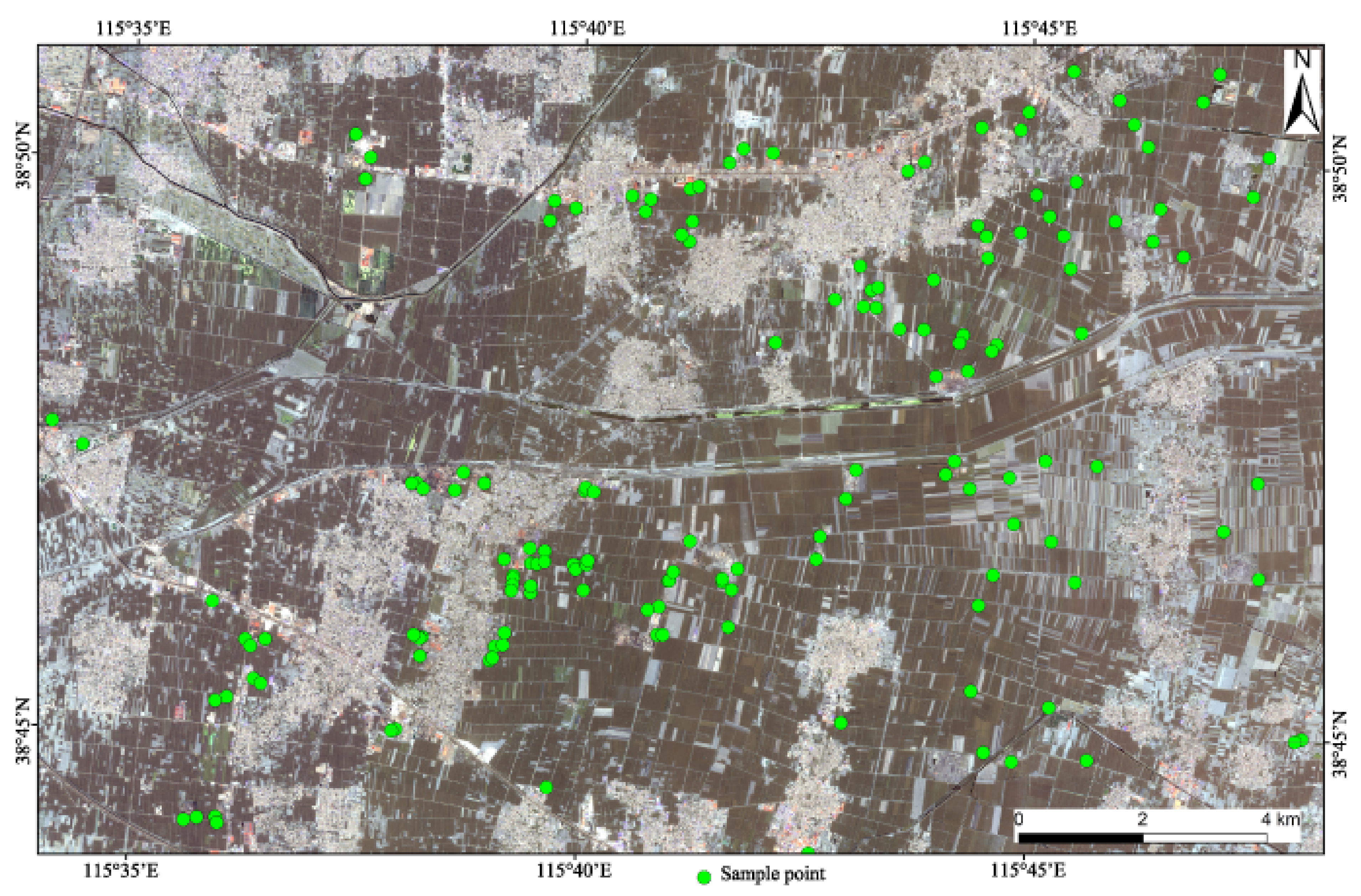
The study area is located at the southwest of Xiongan, which belongs to Anxin County and has a continental semi-humid and semi-arid climate of the warm temperate monsoon type [19]. From September to October, 2019, the process of sampling was conducted on the ground before and after corn harvest; the sampling points were mainly distributed on farmland, and a few of them were located in construction sites and tailings heaps, where 264 samples were collected. The area was about 300 km2 (see Figure 1).

Figure 1.
Distribution of soil sampling sites in the study area.
In order to improve the representativeness of samples, a 0–20 cm plow layer was collected for soil samples, and 5 sub-sampling points were arranged in a plum shape within 50 m of each sampling point. Impurities such as rocks, weeds, and tree roots were removed from the sampling points, and a mixed sample was synthesized by the quartering technique. Samples were stored in polyethylene sample bags weighing more than 1 kg. Then, the longitude and latitude based on the WGS84 coordinate system were used to obtain the positioning coordinates. At the same time, soil characteristics and the surrounding environment were recorded in detail through field investigation.
2.2. Chemical Analyses
At first, 100 mg samples and 1 g sodium peroxide were mixed well in the pyrolytic graphite crucible and then covered by 0.5 g sodium peroxide. Further, the pyrolytic graphite was placed in a porcelain crucible and put into a muffle furnace that was heated to 700 °C until the sample was molten. After cooling, the graphite crucible was put into a beaker containing about 80 mL of boiling water and heated on an electric plate until the melt was completely dissolved. The beaker and precipitate were rinsed with sodium hydroxide solution and the filtrate was discarded. The precipitate was dissolved with hot nitric acid and diluted to 25 mL with nitric acid, which was diluted 10 times with water once again. At last, the contents of REEs were measured by inductively coupled plasma mass spectrometry (ICP-MS) (Nexion 175 350X/Csy-066) [20].
2.3. Spectral Measurements and Transformations
The reflection spectrum of soil samples in the VIR, NIR, and SWIR electromagnetic range (350 nm–2500 nm) was measured by an SVC spectroradiometer with a total of 1024 bands. The spectral resolutions were ≤3.5 nm from 350 nm to 1000 nm, ≤9.5 nm from 1000 nm to 1850 nm, and ≤6.5 nm from 1850 nm to 2500 nm. Before measurement, the sensor was adjusted by a white reference plate; the distance between the spectroradiometer and samples was 5–10 cm, and the field angle was 25°. To minimize measurement errors, five replicates were measured for each soil sample. The average spectrum of the five replicates was used for evaluations. Under the influence of environment, wavelengths less than 400 nm were removed because of the noise of the ultraviolet spectrum, and wavelengths in the range of 400–2500 nm were used, with a total of 924 bands.
The prediction results depended on the pretreatment steps of the reflection spectrum to some extent. To effectively eliminate spectral noise and maintain the chemical information, Savitzky–Golay filtering was used for spectral smoothing [21]. In addition, the baseline effect may have resulted from the particle size rather than chemical composition. In order to enhance the absorption characteristics, the spectra were transformed by standard normal variable (SNV), first-order differential (FD), second-order differential (SD), multiple scattering corrections (MSC), and continuum removal (CR) techniques.
2.3.1. SNV Transformation
Spectral scattering caused by particle size, surface scattering, and optical path variation was eliminated by focusing and scaling. The spectra were standardized by SNV transformation [22].
2.3.2. FD Transformation
The derivative is widely used to correct baseline effects, eliminate non-chemical effects, and establish robust correction models. Some information “hidden” in the spectra may be easily revealed after first or second-order differentiation. FD transformation is just a measure to detect the slope at each point, which is not affected by the pure additive baseline excursion. Therefore, the background interference is minimized, and the method is a very effective technique to eliminate excursion [23].
2.3.3. SD Transformation
SD transformation is a measure to detect the change of a slope, and it is not affected by any linear “skew” except for the removal of pure additive offset. Therefore, SD transformation is efficient enough to remove the baseline offset and slope, and the nearby peaks and sharpen features are clearly distinguished [23].
2.3.4. MSC Transformation
MSC transformation is a modification technique used to compensate for additive and/or multiplicative effects in spectral curves; it is used to eliminate baseline shift and drift between samples and highlight differences. The average reflectance of samples is calculated, and it acts as the standard to obtain the linear shift (regression constant) and oblique offset (regression coefficient). Finally, the linear shift is subtracted from the original spectra and divided by the regression coefficient to obtain the corrected spectra and improve the signal-to-noise ratio (SNR) [24].
2.3.5. CR Transformation
CR transformation is an effective spectral analysis technique used to enhance absorption characteristics; the absorption and reflection characteristics of spectral curves are effectively highlighted, and the reflectance is normalized to 0–1 to extract the characteristics for interpretation [25].
2.4. Modeling for Prediction
In the modeling phase, chemical quantitative analysis with spectral curves is required to establish inversion models which assign the concentration contents or discrete reflectance to spectral characteristics of samples. As a trace element in soil, the contents of REEs are difficult to identify by spectral characteristics. The construction of the model between contents of REEs and the reflection spectrum was begun by multiple linear regressions to select the optimal band subset [26]. Then, PLS with a full spectrum was applied to build the mapping relationship [27,28]. Currently, machine learning models such as random forests and artificial neural networks’ are utilized to further improve the prediction accuracy [29,30]. As a result, linear and nonlinear models are used for the process of prediction. In this study, PLS, RF, and BPNN are applied, and the modeling accuracy is evaluated below.
2.4.1. PLS
PLS is a commonly used statistical model, and its ability is stronger than other multiple linear regression models. An independent variable X is mapped into a new learning space Y, and the direction of the maximum multidimensional variance is explained in Y space [28]. REEs are correlated with spectral reflectance using PLS, and the interaction between VIS-SWIR spectroscopy and PLS for the prediction of REEs is evaluated. PLS is commonly applied to correlate data obtained from hyperspectral images and analyze their corresponding chemical concentration. It is known as a sum of regression analysis, principal component analysis, and correlation analysis.
2.4.2. RF
RF is a predictive model based on classification and regression trees (CART) and the bagging learning strategy [31], where a decision tree is generated from all properties and it is randomly collected from a fixed-size subset of attributes, resulting in a reduced time complexity. In particular, random sampling is repeated K times to generate a fixed number of subsets from all samples, where K is the number of trees in the forest, and only a fixed number of sub-attributes is selected for each sample. Each sample with the corresponding sub-attributes is used to generate a regression tree, and the forest is made up of trees. Finally, the results are achieved by collecting the scores of voting from all of trees.
2.4.3. BPNN
BPNN is a learning model for a multilayer neural network, with the weights and thresholds of the network constantly adjusted through back propagation to minimize the sum of the squared errors; the final output is considered to be as close as possible to the expected output, so it is able to achieve the purpose of training [29]. Based on gradient descent, the model includes two processes: information forward propagation and error backward propagation. The attributes are transmitted from the input layer to output layer when the network acts as a learning process. In addition, the gradient is fed back to adjust the weight and bias of each neuron and minimize the error between predicted and real values if the output does not meet the goal.
3. Results and Discussion
3.1. Analysis of REEs in Soil
Through the preliminary analysis of soil samples in the study area, 264 samples were divided into a calibration set and validation set. The basic characteristics of the 264 samples are shown in Table 1, and the average contents of La, Ce, Nd, Sm, and Y in soil are 40.9, 76.0, 38.4, 6.19, and 27.5 mg/kg respectively, where Ce, Nd, and Sm are slightly lower than the average national contents and La and Y are higher than the average national contents. The average content of REEs is 219.1 mg/kg in the study area, which is slightly higher than the average content of 168 mg/kg in the crust and the average content of 216 mg/kg in Chinese soil. The contents of REEs reported abroad are on the range of 30–700 mg/kg, and the coefficient of variation (C.V.—the standard deviation divided by the mean) is relatively low. If C.V. is less than 1, it indicates that the spatial distribution of REEs is random and uniform and is less affected by human activities.

Table 1.
REE concentration in soil.
3.2. Analysis of Soil Spectra
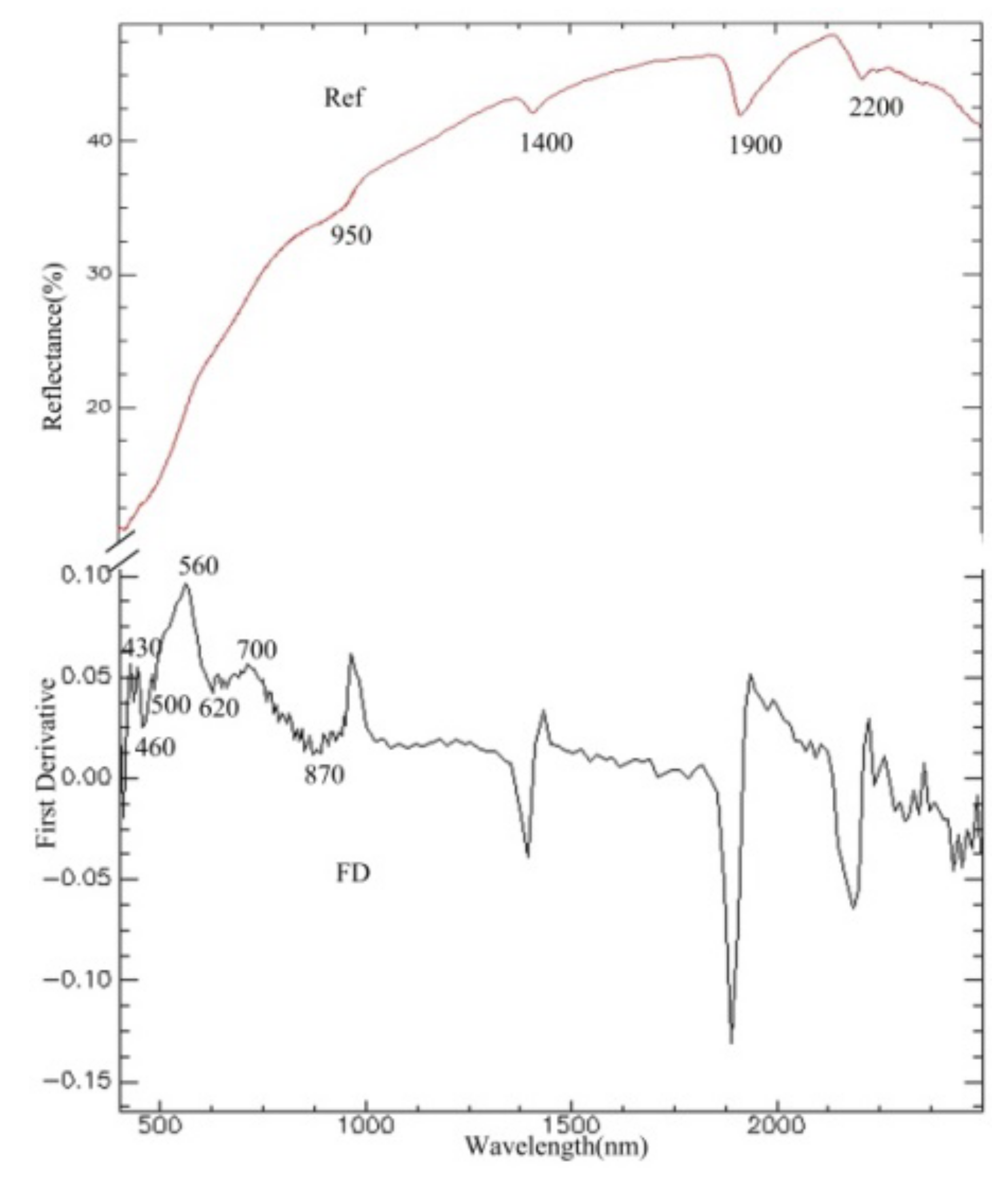
The reflection spectrum and FD transformation of a soil sample in the study area are shown in Figure 2. The reflection spectrum has obvious absorption characteristics near the wavelengths of 1400 nm, 1900 nm, and 2200 nm, which are mainly caused by hydroxyl in free water and lattice hydroxyl in clay minerals. In the visible region, the complexity of absorption characteristics was caused by the absorption of iron; the absorption characteristics from 400–1300 nm were caused by iron in ferric or ferrous forms [32]. The curve for the FD transformation was suitable to study the absorption characteristics of iron oxide, while the absorption peak near 560 nm was caused by hematite, and the weak absorption peak near 430 nm was caused by goethite [33]. The value from 560–760 nm was regarded as corresponding to the absorption characteristics of the total content of Fe2O3 [34]. Studies have found that the reflection spectrum has a broad relationship with organic matter from 400–530 nm, and it is regarded as corresponding to the absorption characteristics of organic matter.

Figure 2.
Measured reflection spectrum and FD transformation.
3.3. Spectral Response for the Contents of REEs
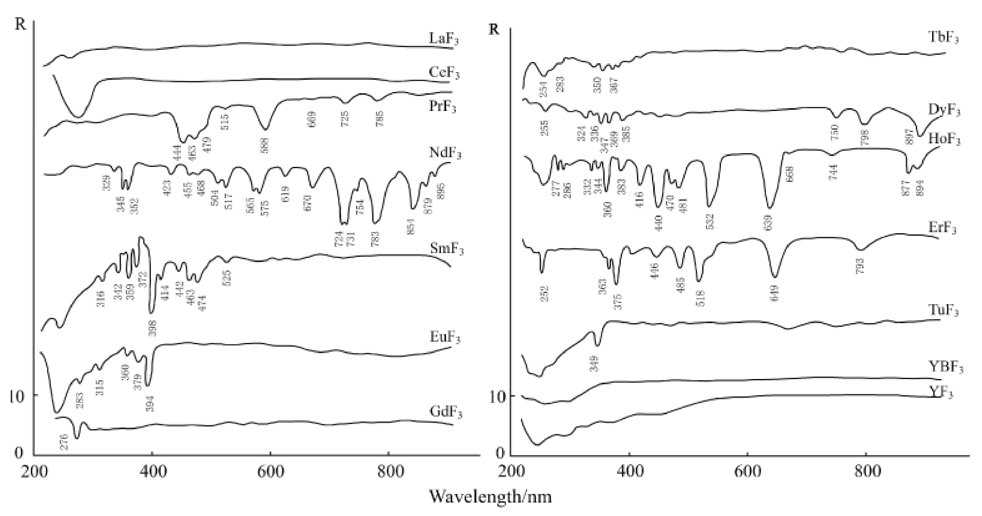
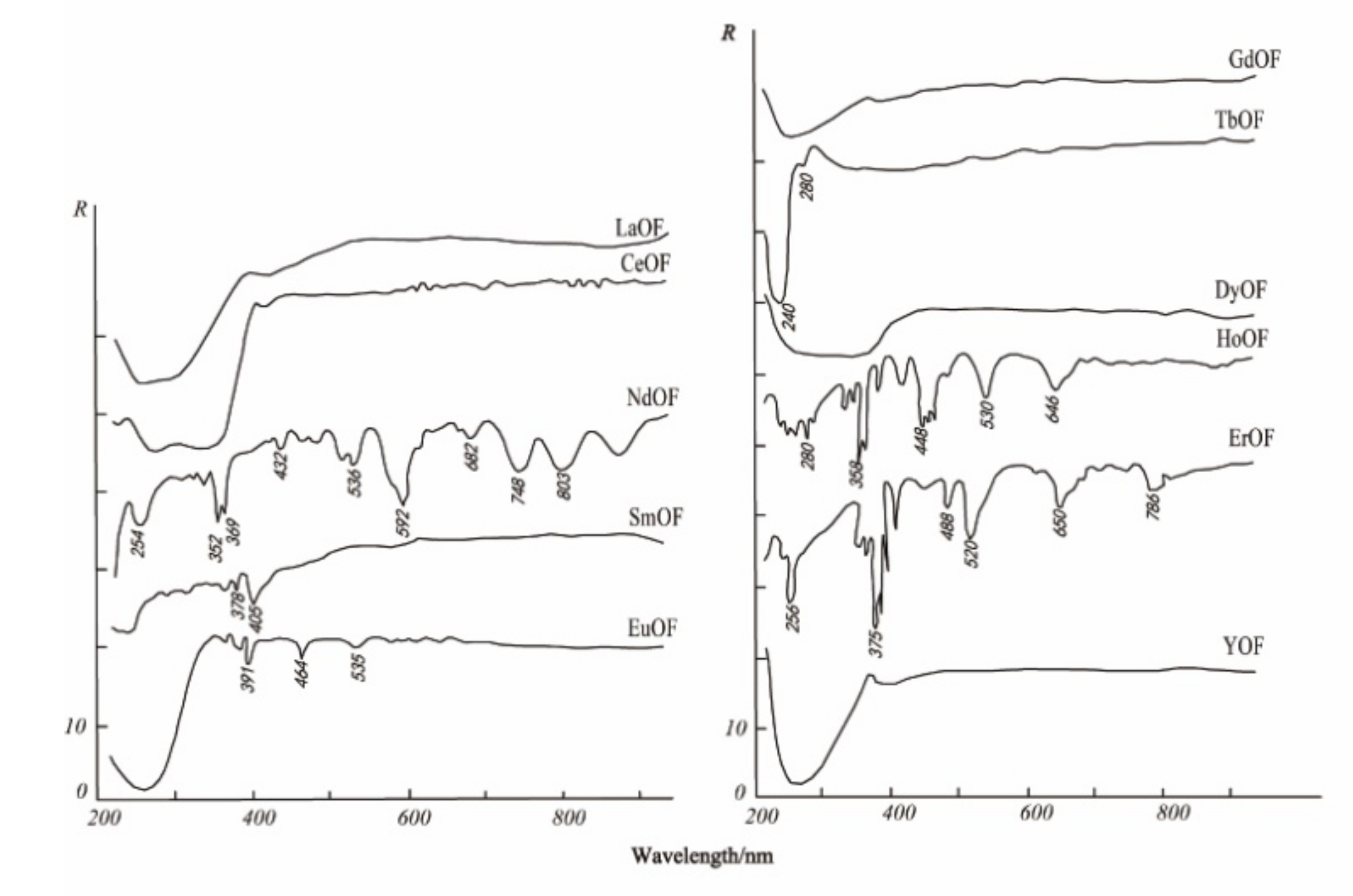
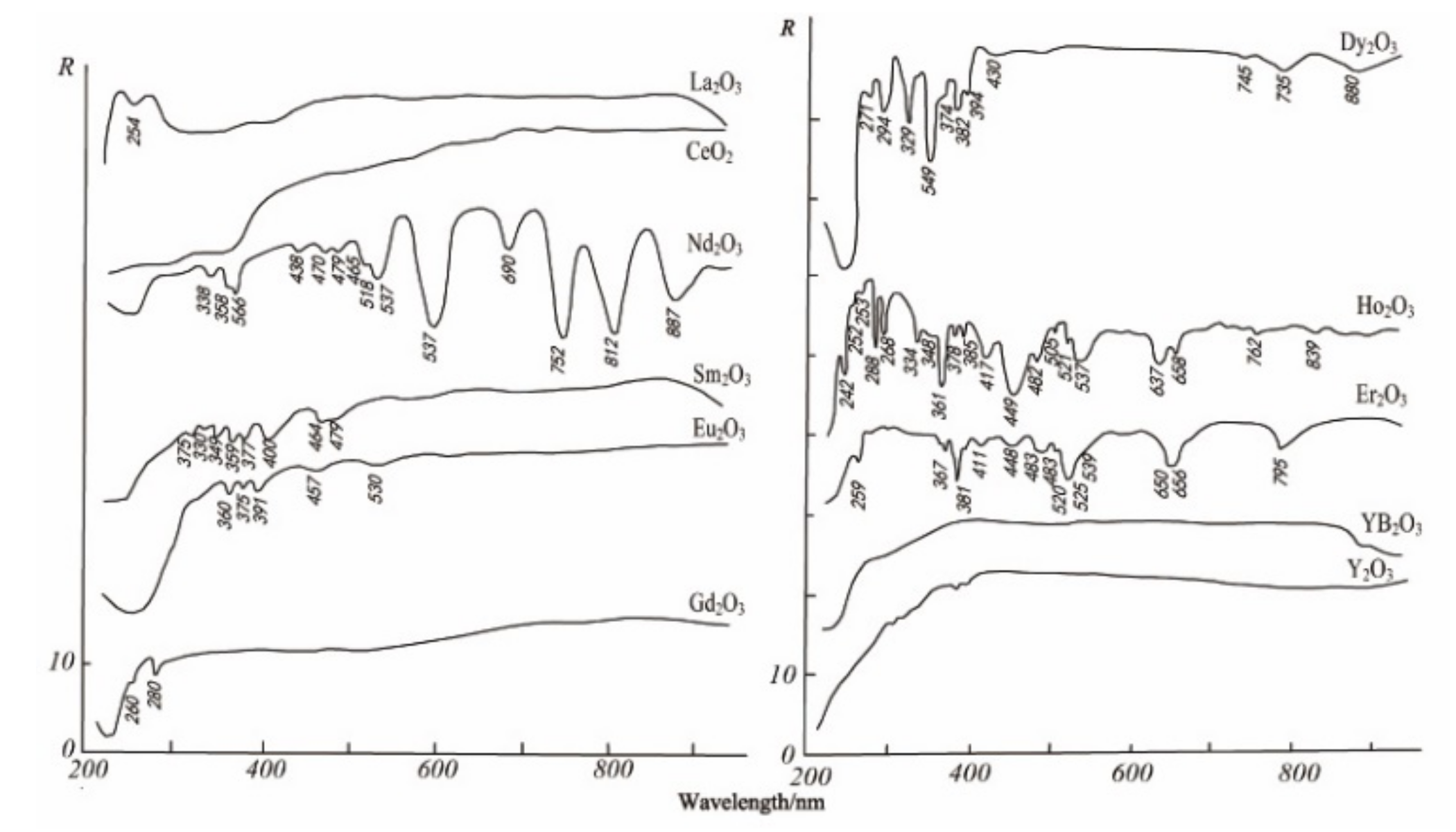
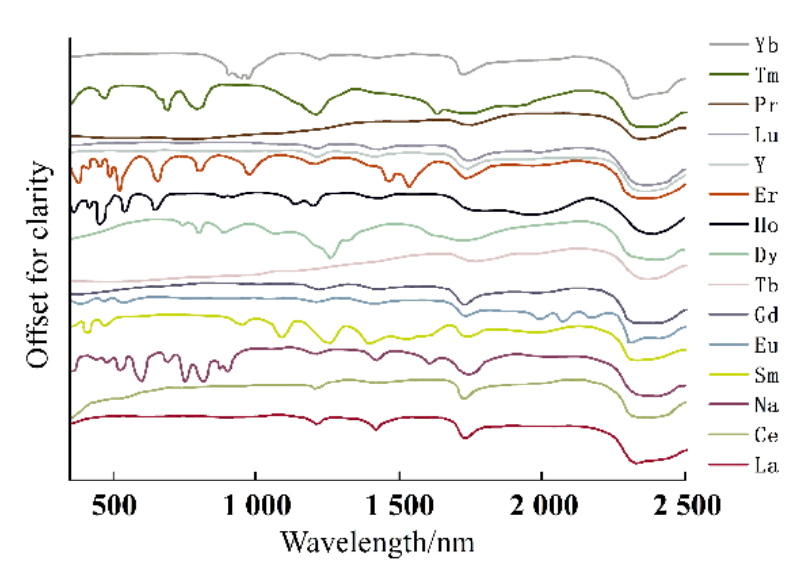
The electronic spectrum of REEs is composed of a series of clear lines that are formed by 4f electron transitions in ultraviolet, visible, and infrared ranges. In addition, the spectral characteristics of studied REEs obviously move to the long-wave range according to the order of fluoride, oxyfluoride, and oxide [35]. Figure 3, Figure 4 and Figure 5 show the spectra of fluoride, oxy-fluoride, and oxide and indicate the frequency of maximum absorption peaks. The compounds containing lanthanides have obvious absorption properties at VIR-SWIR, and the strong absorption of REEs is mainly caused by the electronic transition of 4f-4f configurations. For light fluorocarbons in REEs, most characteristics are attributed to Nd3+, Pr3+, Sm3+, and Eu3+. Dai et al. collected the laboratory spectra of 15 REEs (see Figure 6), and the absorption characteristics of each element were analyzed. The spectrogram of REEs has been added to the latest USGS spectral library [36].
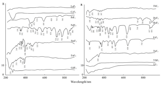
Figure 3.
Electronic spectra of fluorites.

Figure 4.
Electronic spectra of oxy-fluorites.
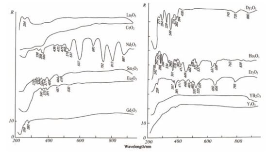
Figure 5.
Electronic spectra of oxides.
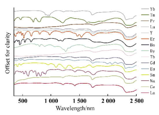
Figure 6.
Electronic spectra of REEs.
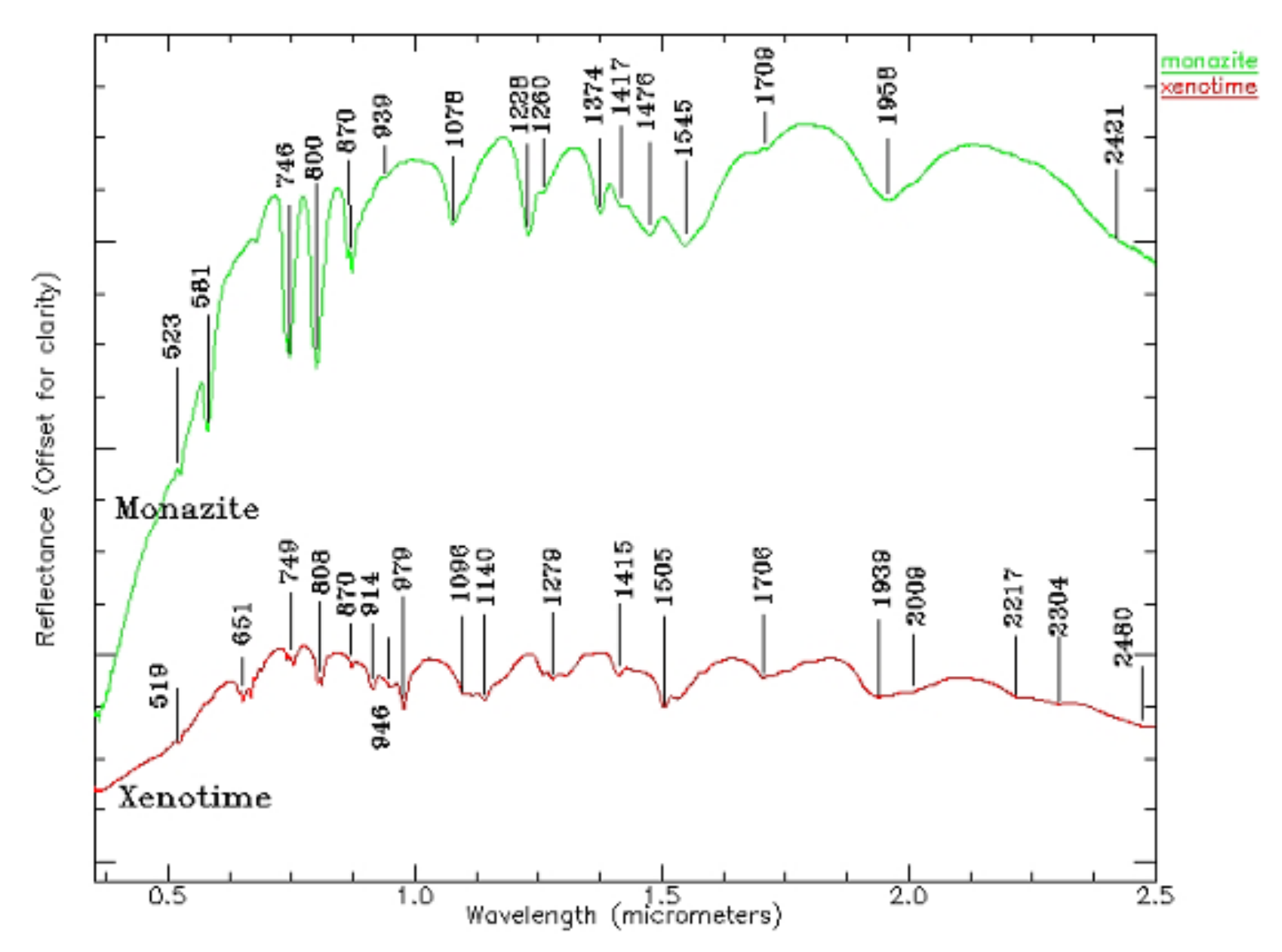
The fluorocarbons mainly include bastnaesite, and parisite, and the phosphates mainly include monazite, Xenotime, britholite, etc. The silicates mainly include cerium silicate, allanite, zircon, etc. [37].
Monazite is a kind of phosphate mineral containing Ce, Y, and La, and the theoretical contents are 34–99% of Ce2O3 and 34.74% of La2O3. The theoretical composition of Y is oxide containing yttrium and erbium (61.4%) and phosphorus pentoxide (38.6%), sometimes containing thorium dioxide, uranium dioxide (5%), and zirconium oxide (3%). There are more than a dozen groups of absorption characteristics for monazite and conch (see Figure 7). The spectral characteristics of monazite mainly reflect the absorption peak of Nd, which is influenced by a small set of Sm and Pr; the spectral characteristics of actinides mainly reflect the absorption peaks of dysprosium, erbium, and ytterbium.
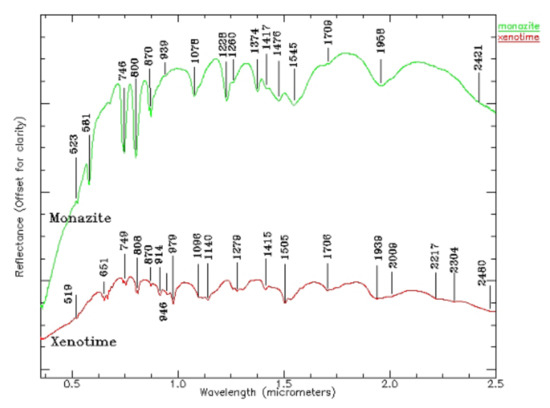
Figure 7.
Electronic spectra of phosphates (monazite and xenotime) (0.5–2.5 µm).
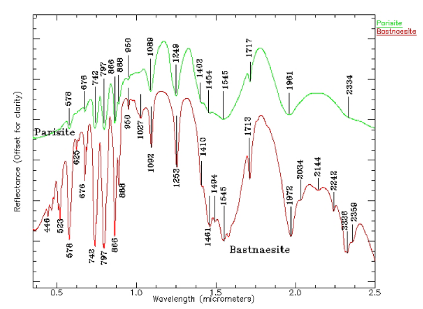
When Ce: La = 1, Ce2O 330.56, La2O 330.33, Co 224.58, CaO 10.44, and F 7 are mainly composed of the Ce group, and the amounts of Ce substituted by REEs such as La, Nd, and Sm are able to reach 1: 1. Bastnasite is a cerium–fluorocarbonate mineral, often occurring with some minerals containing REEs, such as epidote, ceresite, ceresite, etc. There are more than 10 groups of absorption characteristics of fluorine; they are mainly caused by Nd, Sm, Pr, and CO3 (see Figure 8). The reflection spectrum is coincident for La in fluorocarbonates on the whole group, and the position of rare earth cations is very similar for corresponding minerals [38].
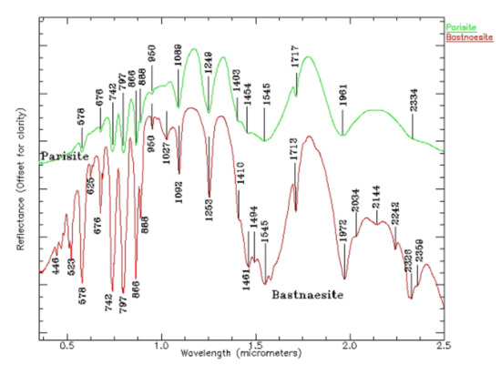
Figure 8.
Electronic spectra of fluorocarbonates (parasite and bastnaesite) (0.5–2.5 µm).
3.4. Modeling Prediction
The proposed technique was implemented with the Matlab 2021a language on a personal computer with a 2.30 GHz CPU and 8.00 G RAM on the Windows 10 operation system. After spectral transformation, PLS, RF, and BPNN were used for inversion modeling, and the results are shown in Table 2. The predicted values were correlated with measured contents according to chemical analysis, and the correlation improved as the R2 moved closer to 1. Moreover, the root mean square error (RMSE), ratio of percent deviation (RPD), and ratio of error range (RER) were utilized to objectively evaluate the performance of different models. RPD is the ratio of standard deviation to RMSE, and an RPD >1.4 indicates that the effect is applicable [39], RER is the ratio of the value range to RMSE, and a higher RER indicates that the model is robust [40].
Table 2.
Experimental results of calibration and validation sets for PLS, RF, and BPNN.
The training accuracy of RF after FD, SD, MSC, SNV, and CR transformations stays at a satisfactory level, and the R2 between the predicted values and measured contents reaches 0.8 for calibration sets, whichis, higher than that of PLS. However, it is difficult for the testing accuracy to satisfy the application, and the R2 between the predicted values and measured contents is lower than 0.7 for validation sets. Further, BPNN is used for modeling, and 10 hidden layers are set to obtain predicted values. REEs act as the trace elements in soil; they are difficult to directly discriminate by their reflection spectra, and the absorption characteristics of the original spectra are enhanced by spectral transformation. After FD transformation, the R2 between the predicted values and measured contents is 0.986, which is the optimal value among spectral transformation techniques. The minimum RMSE is 3.158, the maximum RPD is 2.607, and the RER is greater than 10, reaching 45.004. After SD and SNV transformations, the R2 values between the predicted values and measured contents reached 0.967, 0.940, 0.915, and 0.900 for validation sets, and RMSE values are 6.168, 7.044, 10.187, and 11.297, respectively. According to the results in Table 2, the overall accuracy of BPNN after FD transformation is higher than that of other machine learning models and spectral transformation techniques.
3.5. Distribution Characteristics of REEs
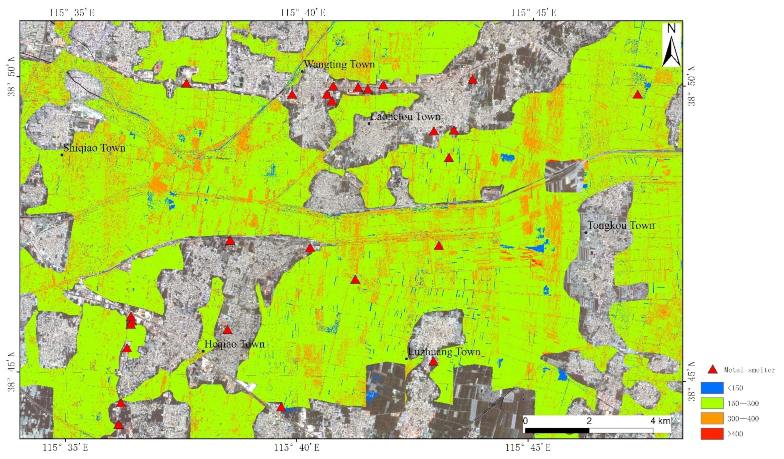
According to the above results, the reasonable model was selected and applied to CASI (Compact Airborne Spectral Imager)/SASI (Short Wave Infrared Airborne Spectral Imager) platforms; that is, iterative training was carried out through FD transformation and BPNN was utilized to build the model. The imaging spectrometer was an aviation hyperspectral imager developed and produced by Canadian ITRES Company. The visible and near-infrared spectral range of CASI is 350–1050 nm and the spectral resolution is 10 nm; the short-wave infrared spectral range of SASI is 950–2500 nm and the spectral resolution is 15 nm. The CASI/SASI airborne hyperspectral imaging system and POS AV410 direction and position system based on DGPS/IMU were mounted on the platform of a Cessna 208 aircraft. CASI images were changed to SASI images and merged into one file with a spectral range of 400–2500 nm; the spatial resolution of each pixel was 2.52 m × 2.52 m, and the number of bands was 173. The content distribution of REEs for the airborne hyperspectral image was mapped by FD transformation and BPNN and is shown in Figure 9, and corresponding evaluation indicators are shown in Table 3.
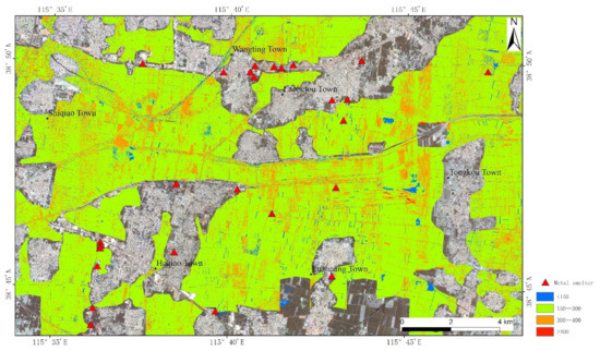
Figure 9.
The content distribution of REEs for airborne hyperspectral image.
Table 3.
Experimental results of FD transformation and BPNN.
The contents of REEs are mainly predicted within the range of 150–400 mg/kg, and the maximum value is 436.2 mg/kg, which basically agrees with the actual situation. REEs tend to concentrate in the upper layers of the soil profile, and the contents of REEs in the soil, especially Ce and Nd, increase with the levels of phosphate. Regions with a red color show high contents of REEs, which is mainly reflected by dust fall from metal smelters, exhaust emissions from vehicle and agricultural fertilization. REEs tend to concentrate in the upper layers of the soil profile, and the concentration of REEs in soil described in the previous studies increased with the levels of phosphate [41]. In addition, REEs have been widely used in agriculture as microfertilizers to improve the quality and yield of agricultural products, but the application in agriculture has enriched soils with hazardous elements [42]. According to Figure 9, the contents of REEs is greater than 400 mg/kg in parts of Tongkou Town; various small smelters are spread here by field investigation, and stringent control measures need to be adopted to make the contents of REEs adhere to the normal level in the regions [43].
4. Conclusions
Soil samples were collected by a SVC spectrometer in the southwest of Xiongan to monitor the contents of REEs in the soil, spectral transformation was utilized to enhance the absorption characteristics of REEs, and machine learning models were used to conduct inversion modeling. The content distributions of REEs were mapped, and the experimental results allow us to make the following conclusions:
- (1)
- FD, MSC, CR, SD, and SNV are used for spectral transformation to eliminate the baseline effect and enhance absorption characteristics. PLS, RF, and BPNN are used to carry out iterative modeling. By comparing the accuracy of various models, it is shown that BPNN has the highest accuracy after FD transformation, and R2 between the predicted values and measured contents is 0.986.
- (2)
- The contents of REEs are 157.3–358.7 mg/kg for soil samples collected at Anxin County, and the reported contents of REEs are in the range of 30–700 mg/kg. The C.V. of REEs is less than 1, which indicates that the spatial distribution of REEs is random and uniform, and it is little affected by human activities.
- (3)
- The average contents of REEs are 261.3 mg/kg for hyperspectral images, which is slightly higher than the average of 207 mg/kg in the crust. It is demonstrated that the control measures are effective, and the contents of REEs satisfy the demands of daily life for most regions of the study area.
Author Contributions
Conceptualization, M.W.; methodology, Z.H. and F.Z.; software, S.L.; data curation, B.N.; validation, W.H. and M.W.; writing—original draft preparation, M.C.; writing—review and editing, Y.Z.; visualization, M.C.; funding acquisition, Z.H. and M.W. All authors have read and agreed to the published version of the manuscript.
Funding
This work is funded by the National Natural Science Foundation of China under Grant Numbers 41901296, 41801394, 41272366, and the Science and Technology Innovation Program of China Metallurgical Geology Bureau under Grant Number CMGB202001.
Institutional Review Board Statement
Not applicable.
Informed Consent Statement
Not applicable.
Data Availability Statement
Not applicable.
Conflicts of Interest
The authors declare no conflict of interest.
References
- Voncken, J.H.L. The Rare Earth Elements: An Introduction; Springer International Publishing: Cham, Switzerland, 2016. [Google Scholar]
- Khan, A.M.; Bakar, N.K.A.; Bakar, A.F.A.; Ashraf, M.A. Chemical speciation and bioavailability of rare earth elements (REEs) in the ecosystem: A review. Environ. Sci. Pollut. Res. 2017, 24, 22764–22789. [Google Scholar] [CrossRef] [PubMed]
- Mikołajczak, P.; Borowiak, K.; Niedzielski, P. Phytoextraction of rare earth elements in herbaceous plant species growing close to roads. Environ. Sci. Pollut. Res. 2017, 24, 14091–14103. [Google Scholar] [CrossRef] [Green Version]
- Chao, Y.; Liu, W.; Chen, Y.; Chen, W.; Zhao, L.; Ding, Q.; Wang, S.; Tang, Y.T.; Zhang, T.; Qiu, R.L. Structure, variation, and co-occurrence of soil microbial communities in abandoned sites of a rare earth elements mine. Environ. Sci. Technol. 2016, 50, 11481–11490. [Google Scholar] [CrossRef]
- Alonso, E.; Sherman, A.M.; Wallington, T.J.; Everson, M.P.; Field, F.R.; Roth, R.; Kirchain, R.E. Evaluating rare earth element availability: A case with revolutionary demand from clean technologies. Environ. Sci. Technol. 2012, 46, 3406–3414. [Google Scholar] [CrossRef] [PubMed]
- Redling, K. Rare Earth Elements in Agriculture with Emphasis on Animal Husbandry. Ph.D. Thesis, LMU, Munich, Germany, 2016. [Google Scholar]
- Chen, Z. The biological hormesis-effects of rare earths and potential effects of application of rare earths on agricultural eco-environment. Rural. Eco-Environ. 2004, 20, 1–8. [Google Scholar]
- Liu, C.; Liu, W.; Huot, H.; Yang, Y.; Guo, M.; Morel, J.L.; Tang, Y.; Qiu, R. Responses of ramie (Boehmeria nivea L.) to increasing rare earth element (REE) concentrations in a hydroponic system. J. Rare Earths 2021. [Google Scholar] [CrossRef]
- Pagano, G.; Guida, M.; Tommasi, F.; Oral, R. Health effects and toxicity mechanisms of rare earth elements—Knowledge gaps and research prospects. Ecotoxicol. Environ. Saf. 2015, 115, 40–48. [Google Scholar] [CrossRef] [PubMed]
- Yuan, Y.; Liu, S.; Wu, M.; Zhong, M.; Shahid, M.Z.; Liu, Y. Effects of topography and soil properties on the distribution and fractionation of REEs in topsoil: A case study in Sichuan Basin, China. Sci. Total Environ. 2021, 791, 148404. [Google Scholar] [CrossRef]
- Chen, H.; Chen, Z.; Chen, Z.; Ou, X.; Chen, J. Calculation of toxicity coefficient of potential ecological risk assessment of rare earth elements. Bull. Environ. Contam. Toxicol. 2020, 104, 582–587. [Google Scholar] [CrossRef]
- Turra, C.; Bacchi, M.A. Evaluation on rare earth elements of Brazilian agricultural supplies. J. Environ. Chem. Ecotoxicol. 2011, 3, 86–92. [Google Scholar]
- Henderson, P. Rare Earth Element Geochemistry; Elsevier: Amsterdam, The Netherlands, 2013. [Google Scholar]
- Bünzli, J.C.G.; Eliseeva, S.V. Basics of Lanthanide Photophysics, Lanthanide Luminescence: Photophysical, Analytical and Biological Aspects; Series on Fluorescence; Springer: Heidelberg, Germany, 2010. [Google Scholar]
- Clark, R.N.; Rencz, A.N. Spectroscopy of rocks and minerals, and principles of spectroscopy. Man. Remote Sens. 1999, 3, 3–58. [Google Scholar]
- Rowan, L.C.; Kingston, M.J.; Crowley, J.K. Spectral reflectance of carbonatites and related alkalic igneous rocks; selected samples from four North American localities. Econ. Geol. 1986, 81, 857–871. [Google Scholar] [CrossRef]
- Zimmermann, R.; Brandmeier, M.; Andreani, L.; Mhopjeni, K.; Gloaguen, R. Remote sensing exploration of Nb-Ta-LREE-enriched carbonatite (Epembe/Namibia). Remote Sens. 2016, 8, 620. [Google Scholar] [CrossRef] [Green Version]
- Boesche, N.K.; Rogass, C.; Lubitz, C.; Brell, M.; Herrmann, S.; Mielke, C.; Tonn, S.; Appelt, O.; Altenberger, U.; Kaufmann, H. Hyperspectral REE (rare earth element) mapping of outcrops—Applications for neodymium detection. Remote Sens. 2015, 7, 5160–5186. [Google Scholar] [CrossRef] [Green Version]
- Wang, Y.; Song, L.; Han, Z.; Liao, Y.; Xu, H.; Zhai, J.; Zhu, R. Climate-related risks in the construction of Xiongan New Area, China. Theor. Appl. Climatol. 2020, 141, 1301–1311. [Google Scholar] [CrossRef]
- Wieser, M.E.; Schwieters, J.B. The development of multiple collector mass spectrometry for isotope ratio measurements. Int. J. Mass Spectrom. 2005, 242, 97–115. [Google Scholar] [CrossRef]
- Savitzky, A.; Golay, M.J.E. Smoothing and differentiation of data by simplified least squares procedures. Anal. Chem. 1964, 36, 1627–1639. [Google Scholar] [CrossRef]
- Kooistra, L.; Wehrens, R.; Leuven, R.S.E.W.; Buydens, L.M.C. Possibilities of visible–near-infrared spectroscopy for the assessment of soil contamination in river floodplains. Anal. Chim. Acta 2001, 446, 97–105. [Google Scholar] [CrossRef]
- Martens, H.; Naes, T. Multivariate Calibration; John Wiley & Sons: Hoboken, NJ, USA, 1992. [Google Scholar]
- Moros, J.; Vallejuelo, S.F.O.D.; Gredilla, A.; Diego, A.D.; Madariaga, J.M.; Garrigues, S.; Guardia, M.D.L. Use of reflectance infrared spectroscopy for monitoring the metal content of the estuarine sediments of the Nerbioi-Ibaizabal River (Metropolitan Bilbao, Bay of Biscay, Basque Country). Environ. Sci. Technol. 2009, 43, 9314–9320. [Google Scholar] [CrossRef] [PubMed]
- Clark, R.N.; Roush, T.L. Reflectance spectroscopy: Quantitative analysis techniques for remote sensing applications. J. Geophys. Res. Solid Earth 1984, 89, 6329–6340. [Google Scholar] [CrossRef]
- Ben-Dor, E.; Banin, A. Near-infrared analysis as a rapid method to simultaneously evaluate several soil properties. Soil Sci. Soc. Am. J. 1995, 59, 364–372. [Google Scholar] [CrossRef]
- Chang, C.W.; Laird, D.; Mausbach, M.J.; Hurburgh, C.R., Jr. Near-infrared reflectance spectroscopy–principal components regression analyses of soil properties. Soil Sci. Soc. Am. J. 2001, 65, 480. [Google Scholar] [CrossRef] [Green Version]
- Wold, S.; Sjöström, M.; Eriksson, L. PLS-regression: A basic tool of chemometrics. Chemom. Intell. Lab. Syst. 2001, 58, 109–130. [Google Scholar] [CrossRef]
- Vijayanand, M.; Varahamoorthi, R.; Kumaradhas, P.; Sivamani, S.; Kulkarni, M.V. Regression-BPNN modelling of surfactant concentration effects in electroless NiB coating and optimization using genetic algorithm. Surf. Coat. Technol. 2021, 409, 126878. [Google Scholar] [CrossRef]
- Ge, Y.; Morgan CL, S.; Wijewardane, N.K. Visible and near-infrared reflectance spectroscopy analysis of soils. Soil Sci. Soc. Am. J. 2020, 84, 1495–1502. [Google Scholar] [CrossRef]
- Breiman, L. Random forests. Mach. Learn. 2001, 45, 5–32. [Google Scholar] [CrossRef] [Green Version]
- Dai, J.; Wu, Y.; Ling, T. Reflectance Spectroscopy and Hyperspectral Detection of Rare Earth Element. Spectrosc. Spectr. Anal. 2018, 38, 3801–3808. [Google Scholar]
- Balsam, W.L. Sediment dispersal in the Atlantic Ocean: Evaluation by visible light spectra. Rev. Aquat. Sci. 1991, 4, 411–447. [Google Scholar]
- Xia, X.Q.; Mao, Y.Q.; Ji, J.F.; Ma, H.R.; Chen, J.; Liao, Q.L. Reflectance spectroscopy study of Cd contamination in the sediments of the Changjiang River, China. Environ. Sci. Technol. 2007, 41, 3449–3454. [Google Scholar] [CrossRef]
- Batsanov, S.S.; Derbeneva, S.S.; Batsanova, L.R. Electronic spectra of fluorides, oxyfluorides, and oxides of rare-earth metals. J. Appl. Spectrosc. 1969, 10, 240–242. [Google Scholar] [CrossRef]
- Raymond, F.K.; Roger, N.C.; Gregg, A.S. USGS Spectral Library. 2017. Available online: https://pubs.er.usgs.gov/publication/ds1035 (accessed on 3 November 2021).
- Dostal, J. Rare earth element deposits of alkaline igneous rocks. Resources 2017, 6, 34. [Google Scholar] [CrossRef]
- Turner, D.J.; Rivard, B.; Groat, L.A. Visible and short-wave infrared reflectance spectroscopy of REE fluorocarbonates. Am. Mineral. 2014, 99, 1335–1346. [Google Scholar] [CrossRef]
- Malley, D.F.; Williams, P.C. Use of near-infrared reflectance spectroscopy in prediction of heavy metals in freshwater sediment by their association with organic matter. Environ. Sci. Technol. 1997, 31, 3461–3467. [Google Scholar] [CrossRef]
- Rossel, R.A.V.; McGlynn, R.N.; McBratney, A.B. Determining the composition of mineral-organic mixes using UV–vis–NIR diffuse reflectance spectroscopy. Geoderma 2006, 137, 70–82. [Google Scholar] [CrossRef]
- Mleczek, P.; Borowiak, K.; Budka, A.; Niedzielski, P. Relationship between concentration of rare earth elements in soil and their distribution in plants growing near a frequented road. Environ. Sci. Pollut. Res. 2018, 25, 23695–23711. [Google Scholar] [CrossRef] [Green Version]
- Ding, S.; Liang, T.; Zhang, C.; Yan, J.; Zhang, Z.; Sun, Q. Role of ligands in accumulation and fractionation of rare earth elements in plants. Biol. Trace Elem. Res. 2005, 107, 73–86. [Google Scholar] [CrossRef] [Green Version]
- Yang, Z.; Li, B.; Li, G.; Wang, W. Nutrient elements and heavy metals in the sediment of Baiyangdian and Taihu Lakes: A comparative analysis of pollution trends. Front. Agric. China 2007, 1, 203–209. [Google Scholar] [CrossRef]
Publisher’s Note: MDPI stays neutral with regard to jurisdictional claims in published maps and institutional affiliations. |
© 2021 by the authors. Licensee MDPI, Basel, Switzerland. This article is an open access article distributed under the terms and conditions of the Creative Commons Attribution (CC BY) license (https://creativecommons.org/licenses/by/4.0/).