
Soil Erosion Susceptibility Prediction in Railway Corridors Using RUSLE, Soil Degradation Index and the New Normalized Difference Railway Erosivity Index (NDReLI)


Abstract
:
1. Introduction
2. Materials and Methods
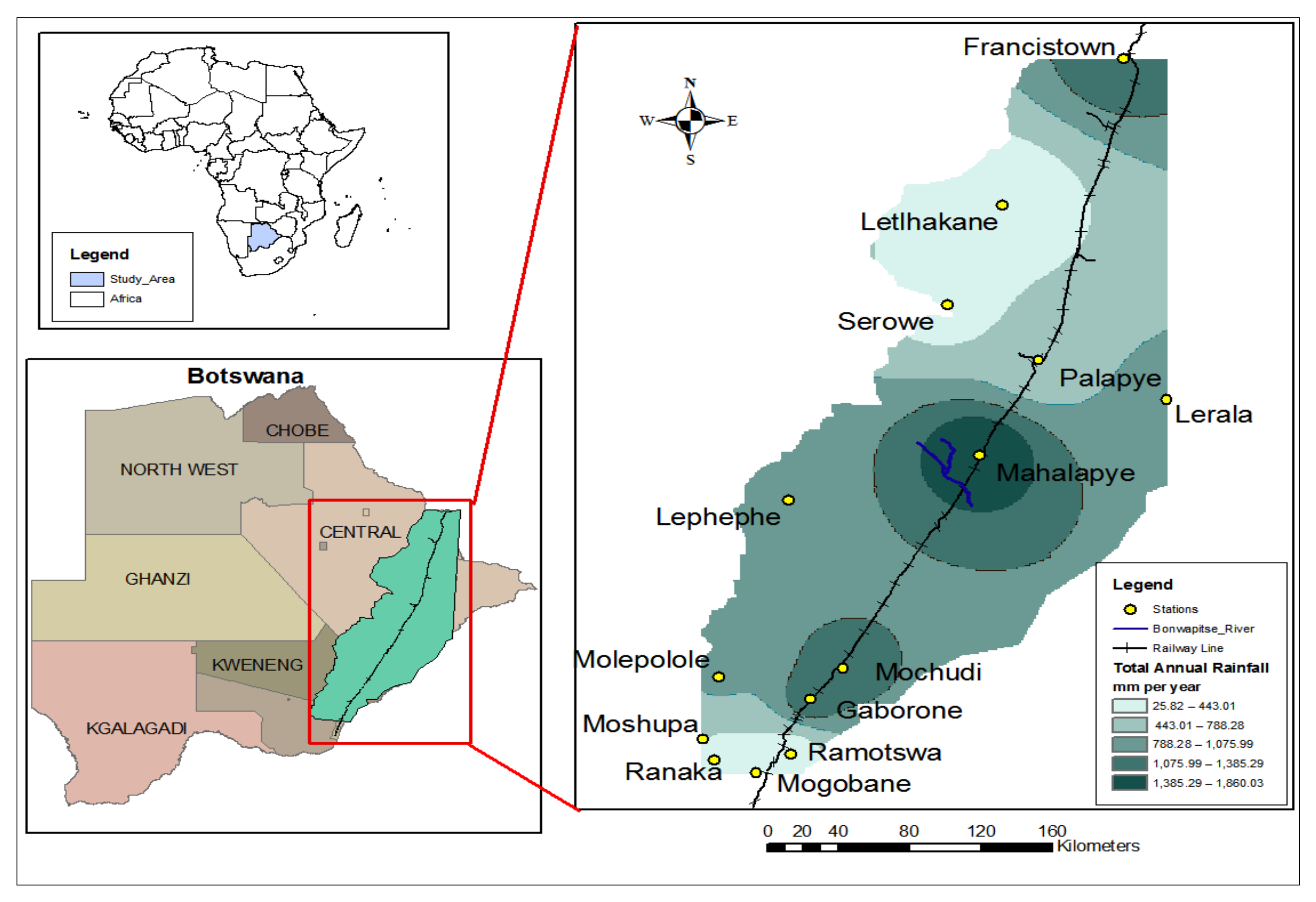
2.1. Study Area
2.2. Data
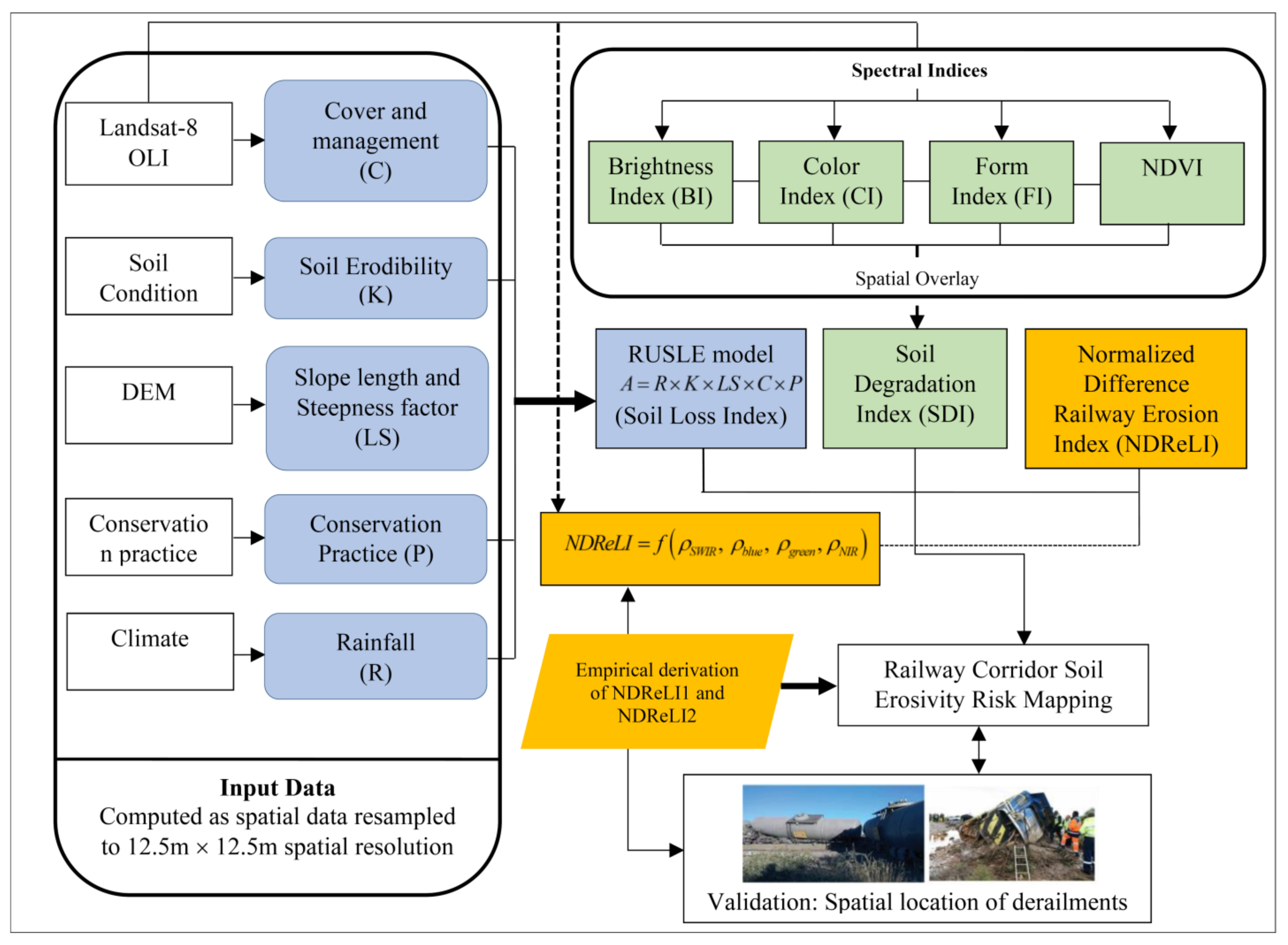
2.3. Methods
2.3.1. Revised Universal Soil Loss Equation (RUSLE)
- Rainfall Erosivity (R-Factor)
- 2.
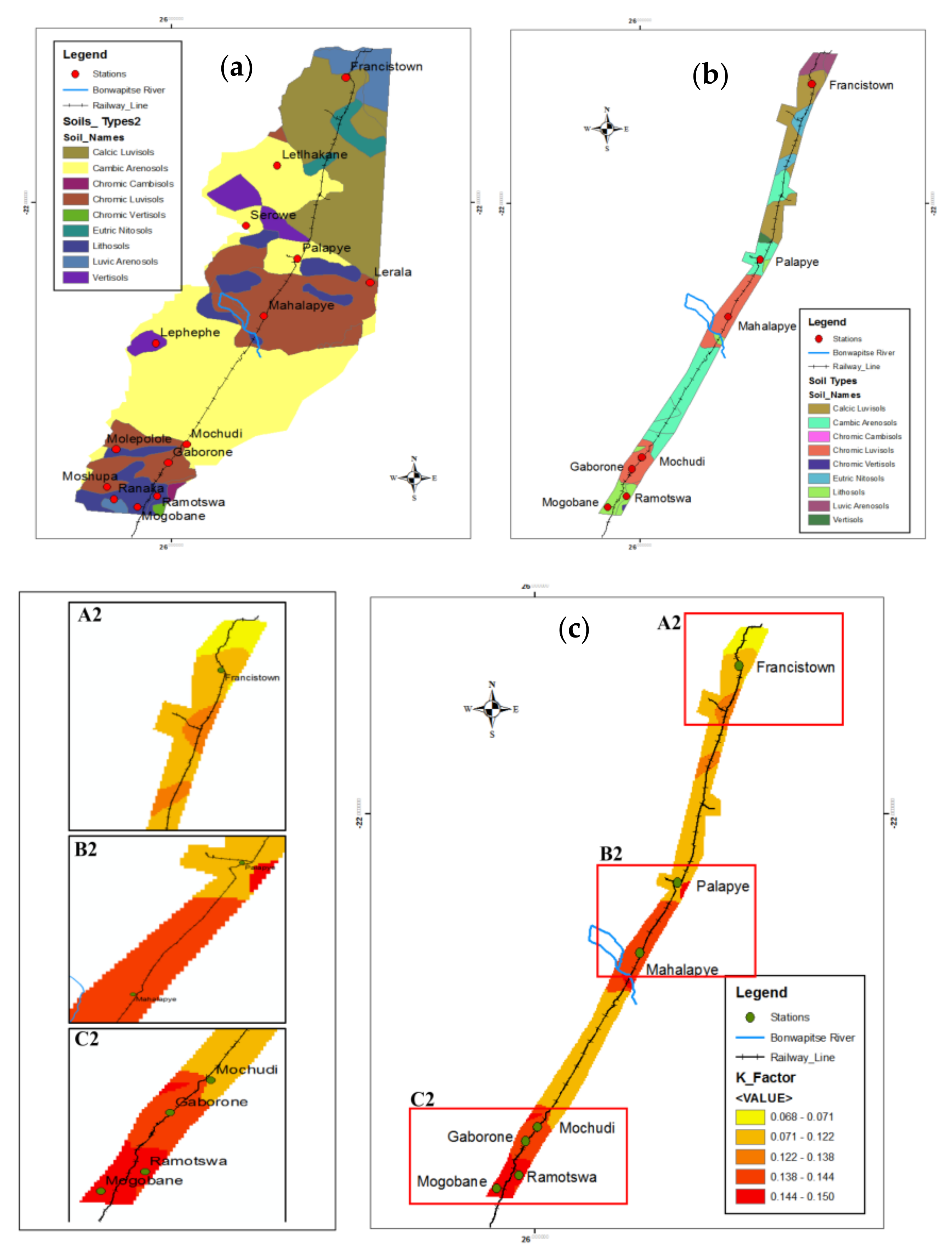
- Soil Erodibility (K-Factor)
- 3.
- Slope Length and Steepness (LS) Factor
- 4.
- Conservation Practice (P-Factor)
- 5.
- Land Cover and Management (C-Factor)
2.3.2. Soil Degradation Index
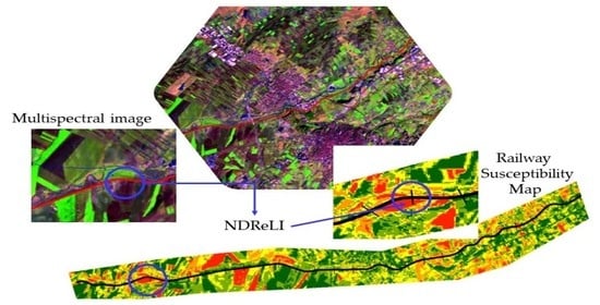
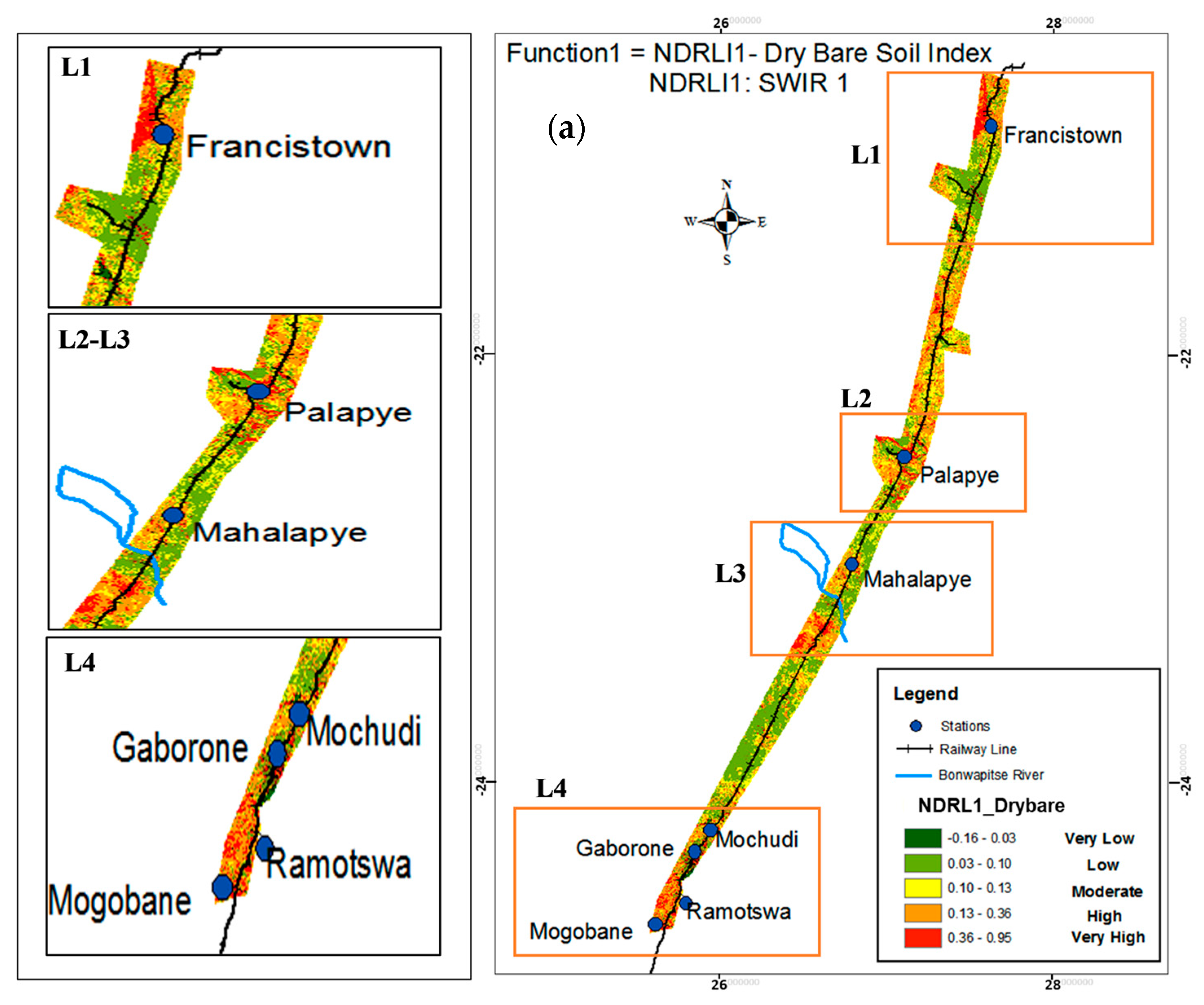
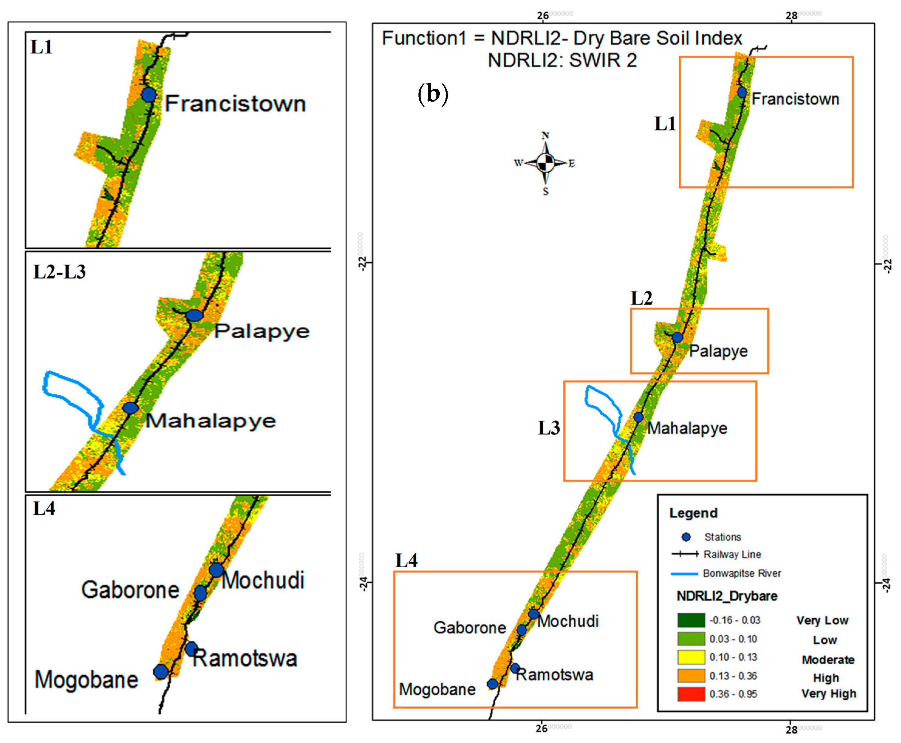
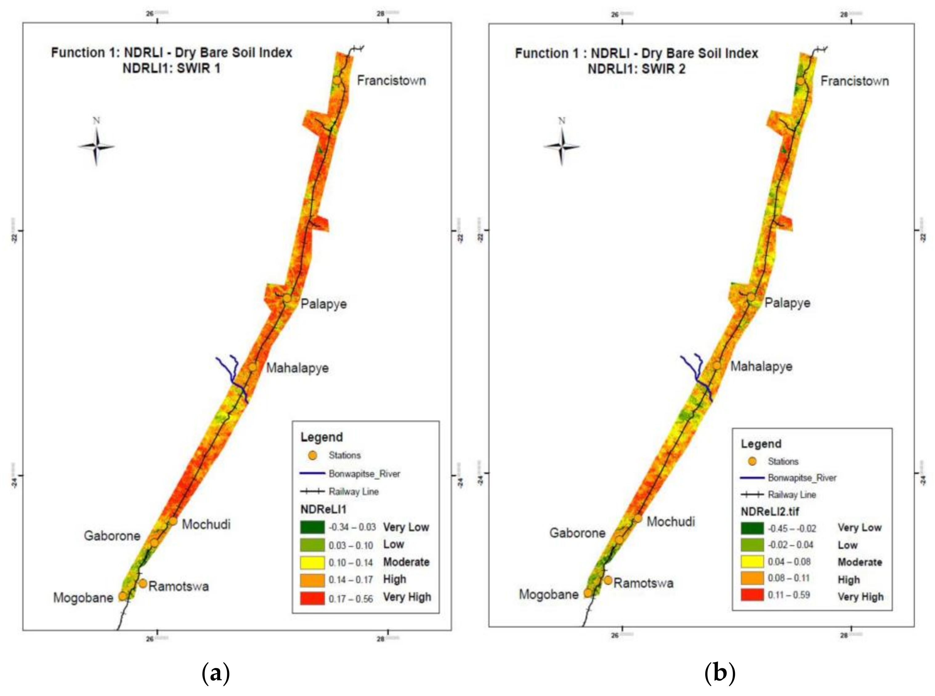
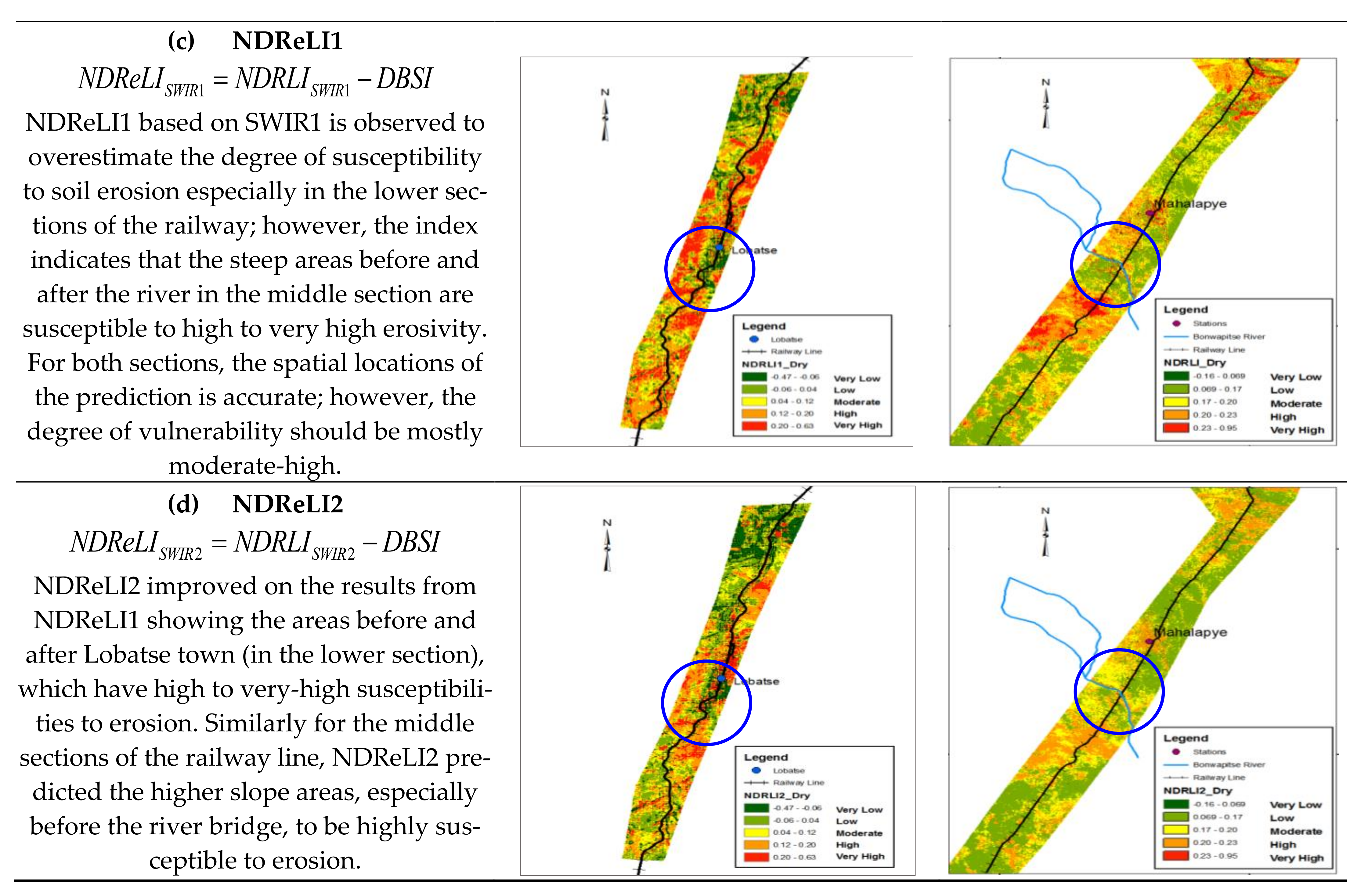
2.3.3. Normalized Difference Railway Erosion Index (NDReLI)
3. Results
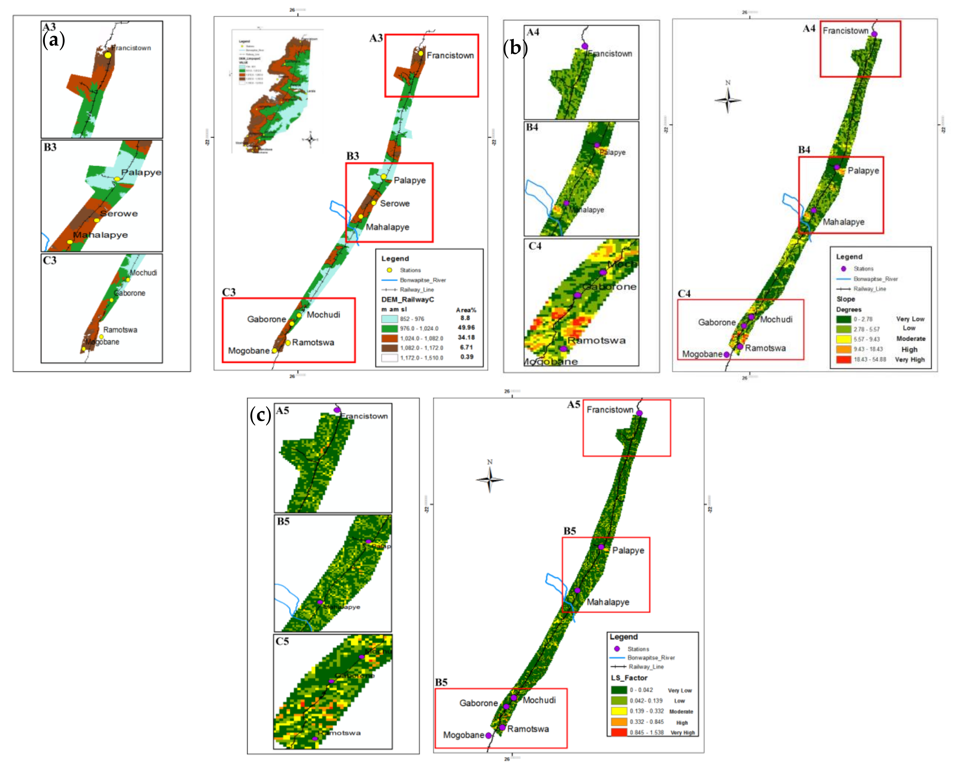
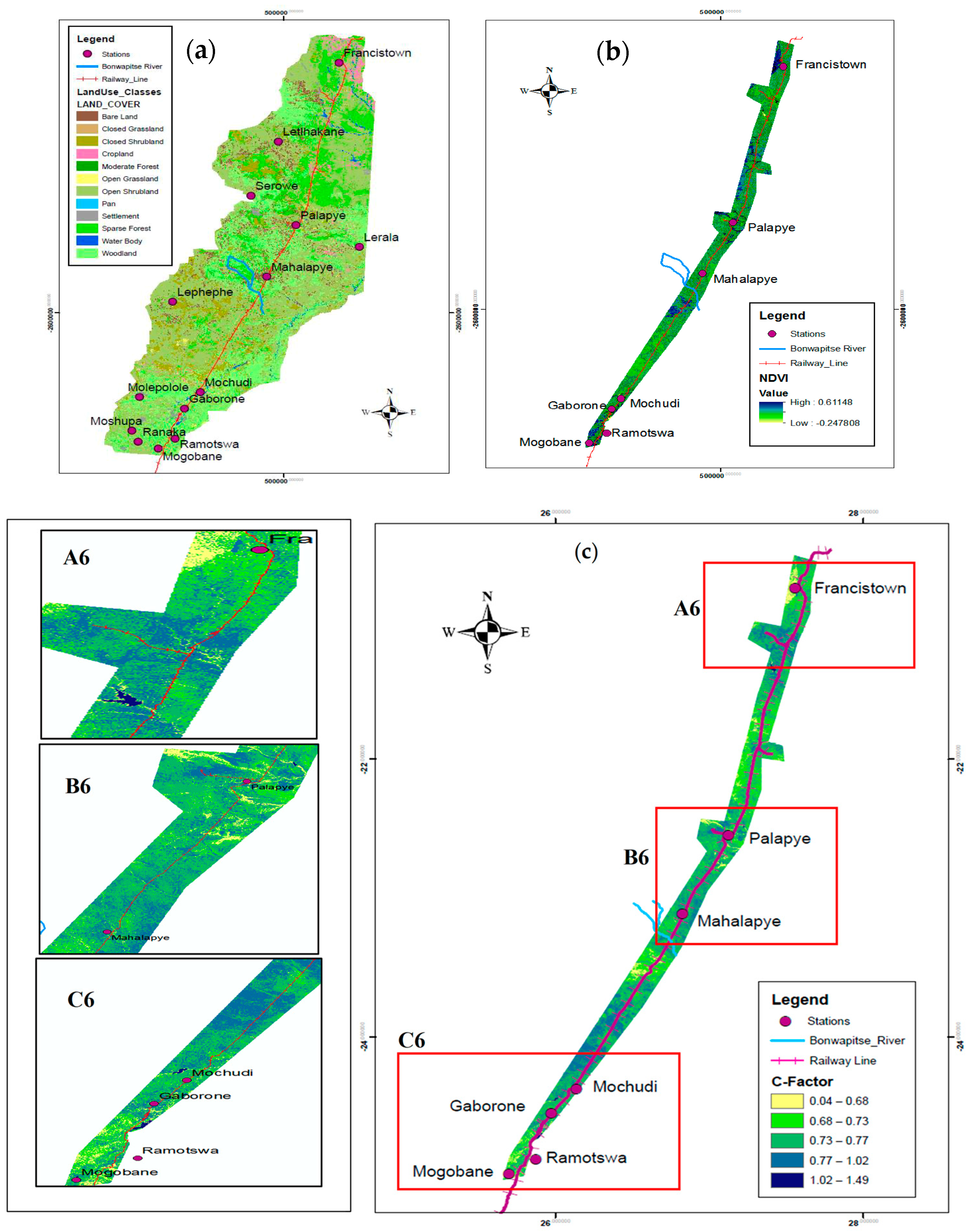
3.1. Soil Erosion Factors for RUSLE Model
3.1.1. R-Factor
3.1.2. K-Factor
3.1.3. Slope Length (L) and Slope Steepness (S) Factor
3.1.4. C-Factor
3.1.5. P-Factor
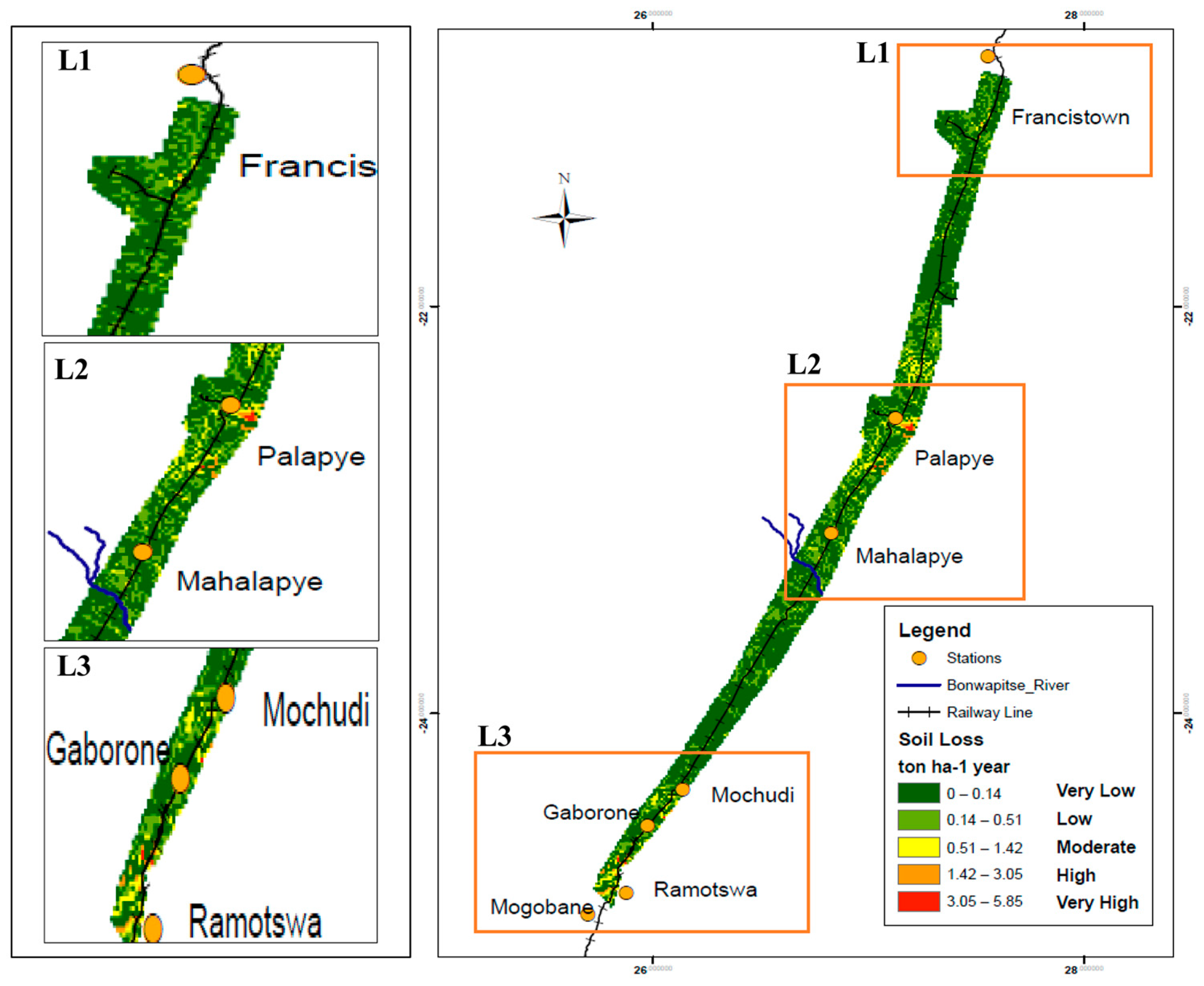
3.2. Mean Annual Soil Loss Using RUSLE
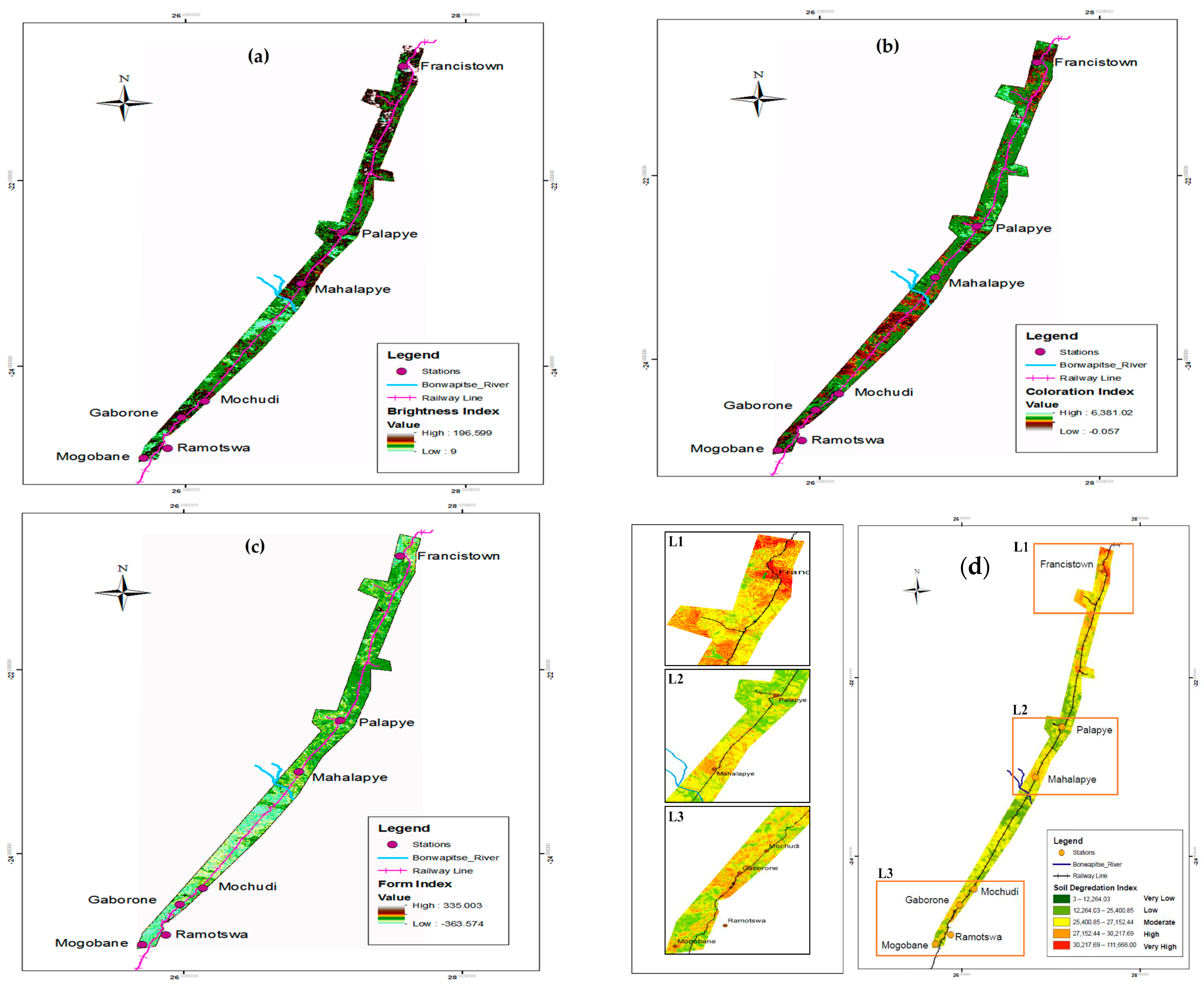
3.3. Soil Degradation Index (SDI) Using Spectral Indices
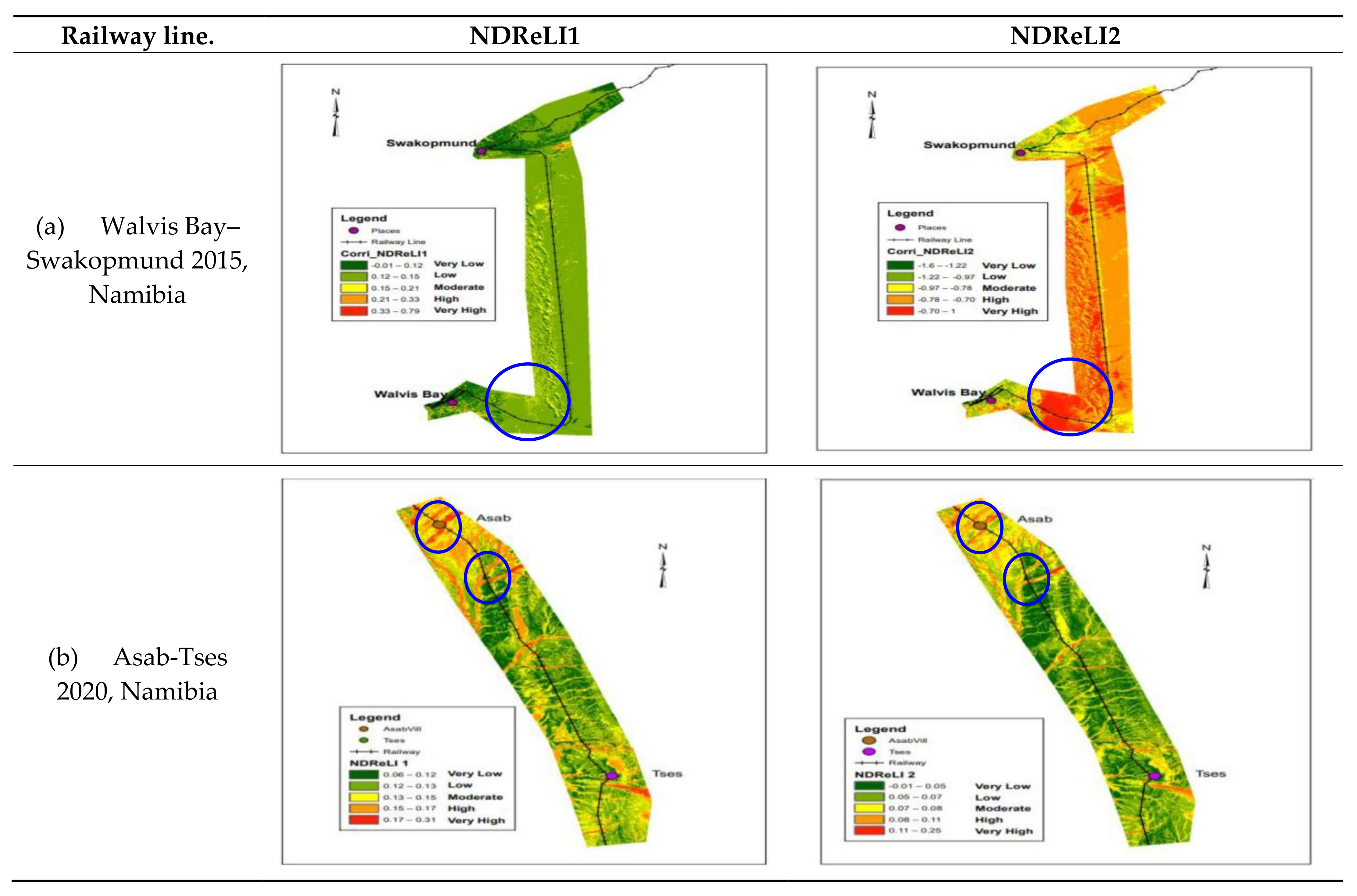
3.4. NDReLI
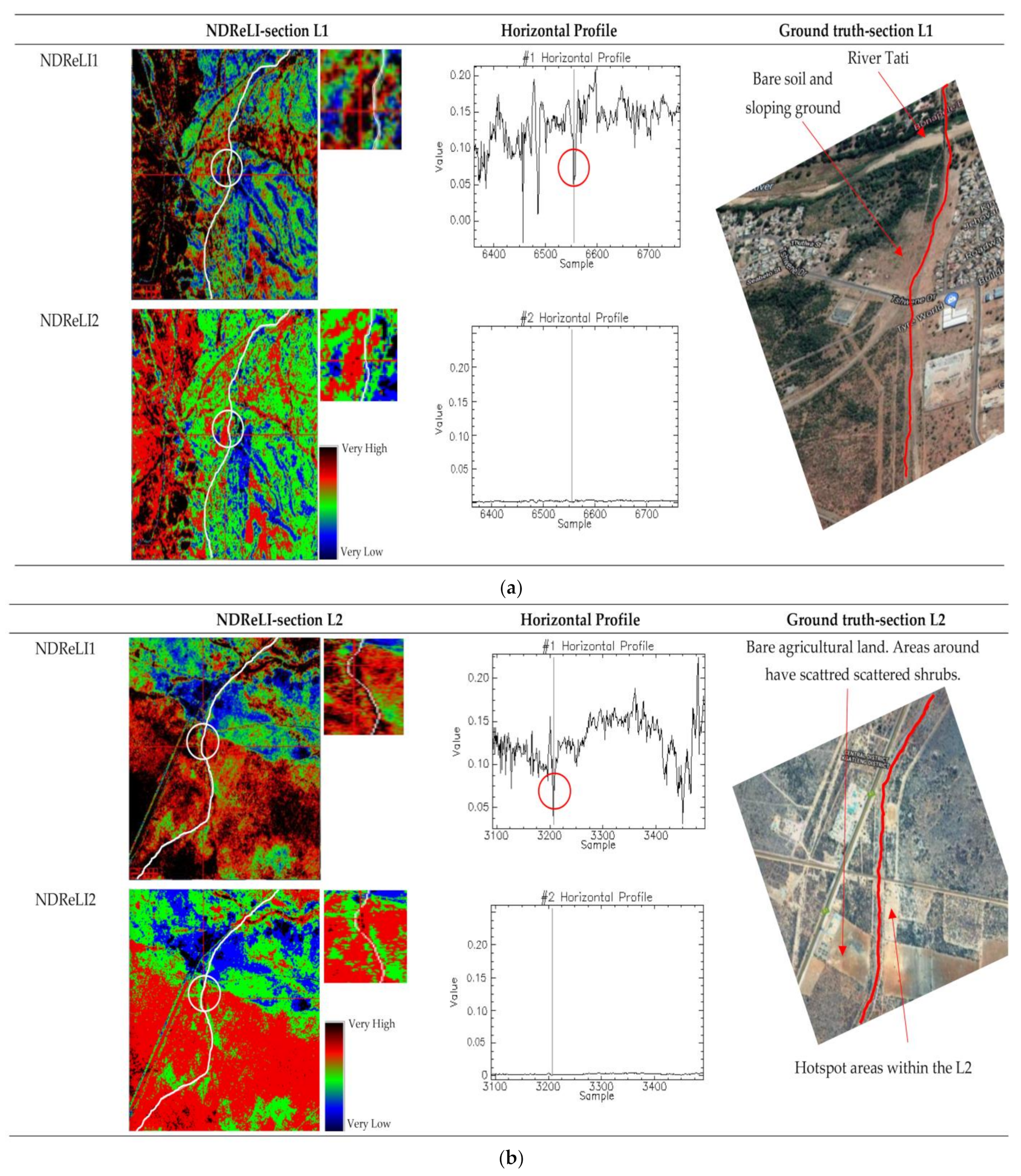
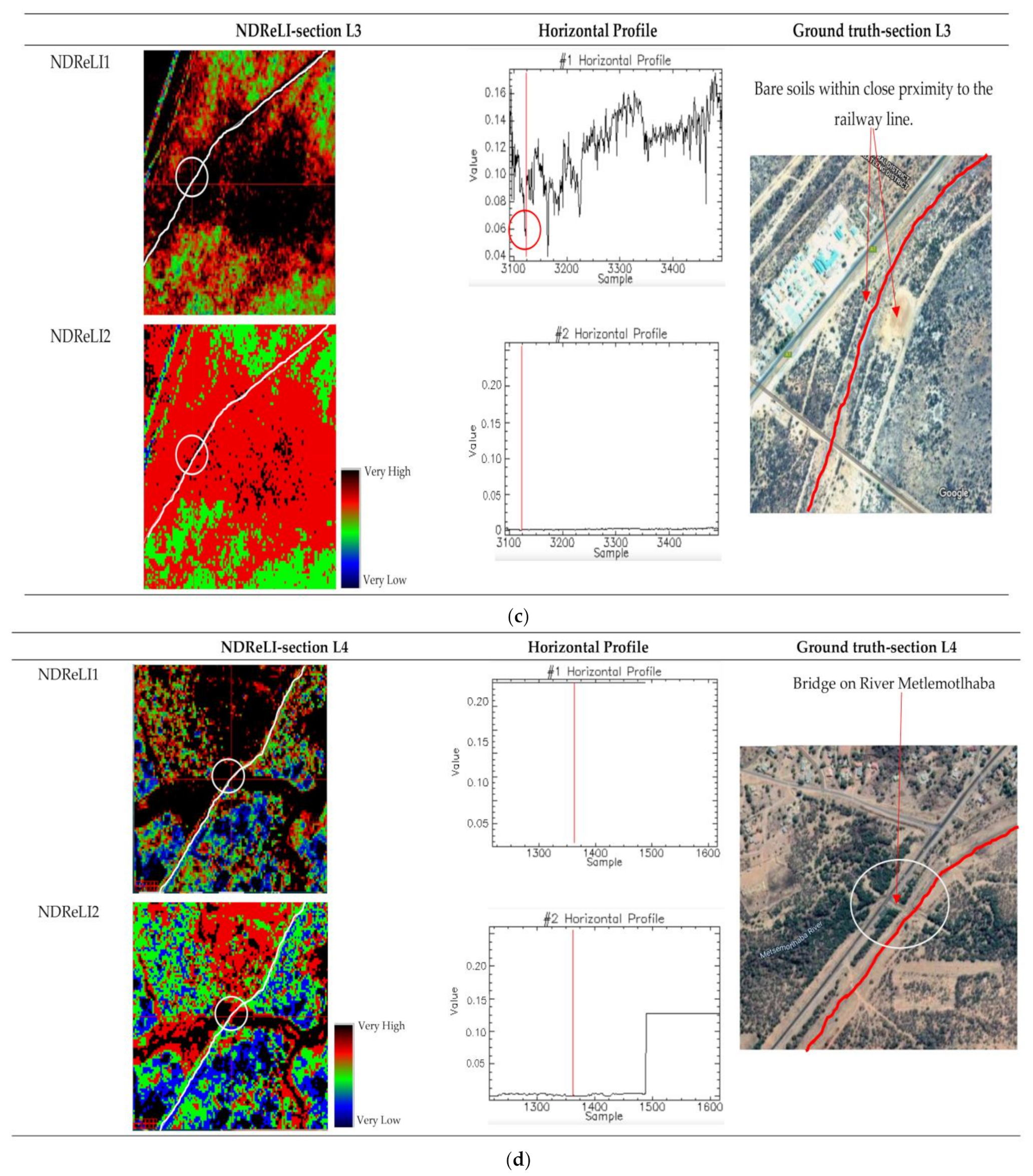
3.5. Empirical Validation and Comparisons of RUSLE, SDI and NDReLI
4. Discussions
5. Conclusions
Author Contributions
Funding
Data Availability Statement
Conflicts of Interest
References
- Özşahin, E.; Duru, U.; Eroğlu, I. Land Use and Land Cover Changes (LULCC), a Key to Understand Soil Erosion Intensities in the Maritsa Basin. Water 2018, 10, 335. [Google Scholar] [CrossRef] [Green Version]
- Borrelli, P.; Robinson, D.A.; Panagos, P.; Lugato, E.; Yang, J.E.; Alewell, C.; Wuepper, D.; Montanarella, L.; Ballabio, C. Land use and climate change impacts on global soil erosion by water (2015–2070). Proc. Natl. Acad. Sci. USA 2020, 117, 21994–22001. [Google Scholar] [CrossRef]
- Tamene, L.; Adimassu, Z.; Ellison, J.; Yaekob, T.; Woldearegay, K.; Mekonnen, K.; Thorne, P.; Le, Q.B. Mapping soil erosion hotspots and assessing the potential impacts of land management practices in the highlands of Ethiopia. Geomorphology 2017, 292, 153–163. [Google Scholar] [CrossRef]
- Pal, S.; Arabameri, A.; Blaschke, T.; Chowdhuri, I.; Saha, A.; Chakrabortty, R.; Lee, S.; Band, S. Ensemble of Machine-Learning Methods for Predicting Gully Erosion Susceptibility. Remote Sens. 2020, 12, 3675. [Google Scholar] [CrossRef]
- Chalise, D.; Kumar, L.; Kristiansen, P. Land Degradation by Soil Erosion in Nepal: A Review. Soil Syst. 2019, 3, 12. [Google Scholar] [CrossRef] [Green Version]
- Ferreira, V.; Panagopoulos, T. Seasonality of Soil Erosion under Mediterranean Conditions at the Alqueva Dam Watershed. Environ. Manag. 2014, 54, 67–83. [Google Scholar] [CrossRef]
- Shikangalah, R.; Paton, E.; Jetlsch, F.; Blaum, N. Quantification of areal extent of soil erosion in dryland urban areas: An example from Windhoek, Namibia. Cities Environ. (CATE) 2017, 10, 8. [Google Scholar]
- Ganasri, B.P.; Ramesh, H. Assessment of soil erosion by RUSLE model using remote sensing and GIS—A case study of Nethravathi Basin. Geosci. Front. 2016, 7, 953–961. [Google Scholar] [CrossRef] [Green Version]
- Food and Agriculture Organization of the United Nations; Intergovernmental Technical Panel on Soils. Status of the World’s Soil Resources (SWSR)–Main Report; Food and Agriculture Organization of the United Nations and Intergovernmental Technical Panel on Soils: Rome, Italy, 2015; Volume 650. [Google Scholar]
- Borrelli, P.; Robinson, D.A.; Fleischer, L.R.; Lugato, E.; Ballabio, C.; Alewell, C.; Meusburger, K.; Modugno, S.; Schütt, B.; Ferro, V.; et al. An assessment of the global impact of 21st century land use change on soil erosion. Nat. Commun. 2017, 8, 2013. [Google Scholar] [CrossRef] [Green Version]
- IPCC. Climate Change and Land: An IPCC Special Report on Climate Change, Desertification, Land Degradation, Sustainable Land Management, Food Security, and Greenhouse gas Fluxes in Terrestrial Ecosystems—Summary for Policy Makers; Report; IPCC: Geneva, Switzerland, 2019. [Google Scholar]
- Merritt, W.; Letcher, R.; Jakeman, A. A review of erosion and sediment transport models. Environ. Model. Softw. 2003, 18, 761–799. [Google Scholar] [CrossRef]
- Ranzi, R.; Le, T.H.; Rulli, M.C. A RUSLE approach to model suspended sediment load in the Lo river (Vietnam): Effects of reservoirs and land use changes. J. Hydrol. 2012, 422–423, 17–29. [Google Scholar] [CrossRef]
- Wischmeier, W.H.; Smith, D.D. Predicting Rainfall Erosion Losses: A Guide to Conservation Planning; No. 537; Department of Agriculture, Science and Education Administration: Washington, DC, USA, 1978. [Google Scholar]
- Renard, K.G. Predicting Soil Erosion by Water: A Guide to Conservation Planning with the Revised Universal Soil Loss Equation (RUSLE); United States Government Printing: Washington DC, USA, 1997.
- Laflen, J.M.; Lane, L.J.; Foster, G.R. WEPP: A new generation of erosion prediction technology. J. Soil Water Conserv. 1991, 46, 34–38. [Google Scholar] [CrossRef]
- Arnold, J.G.; Srinivasan, R.; Muttiah, R.S.; Williams, J.R. Large area hydrologic modeling and assessment, part 1: Model development. J. Am. Water Resources Assoc. 1998, 34, 73–89. [Google Scholar] [CrossRef]
- Kumar, P.S.; Praveen, T.; Prasad, M.A. Simulation of Sediment Yield Over Un-gauged Stations Using MUSLE and Fuzzy Model. Aquat. Procedia 2015, 4, 1291–1298. [Google Scholar] [CrossRef]
- Wang, G.; Gertner, G.; Fang, S.; Anderson, A.B. Mapping Multiple Variables for Predicting Soil Loss by Geostatistical Methods with TM Images and a Slope Map. Photogramm. Eng. Remote Sens. 2003, 69, 889–898. [Google Scholar] [CrossRef]
- Raza, A.; Ahrends, H.; Habib-Ur-Rahman, M.; Gaiser, T. Modeling Approaches to Assess Soil Erosion by Water at the Field Scale with Special Emphasis on Heterogeneity of Soils and Crops. Land 2021, 10, 422. [Google Scholar] [CrossRef]
- Ahmadi, M.; Minaei, M.; Ebrahimi, O.; Nikseresht, M. Evaluation of WEPP and EPM for improved predictions of soil erosion in mountainous watersheds: A case study of Kangir River basin, Iran. Model. Earth Syst. Environ. 2020, 6, 2303–2315. [Google Scholar] [CrossRef]
- Lu, D.; Li, G.; Valladares, G.S.; Batistella, M. Mapping soil erosion risk in Rondônia, Brazilian Amazonia: Using RUSLE, remote sensing and GIS. Land Degrad. Dev. 2004, 15, 499–512. [Google Scholar] [CrossRef]
- Li, X.; Wu, B.; Wang, H.; Zhang, J. Regional soil erosion risk assessment in Hai Basin. Yaogan Xuebao J. Remote Sens. 2011, 15, 372–387. [Google Scholar]
- Le Roux, J.J.; Sumner, P.D. Factors controlling gully development: Comparing continuous and discontinuous gullies. Land Degrad. Dev. 2011, 23, 440–449. [Google Scholar] [CrossRef] [Green Version]
- US Department of Agriculture (USDA). Soil Quality—Urban Technical Note No. 1, Erosion and Sedimentation on Construction Sites; US Department of Agriculture: Washington, DC, USA, 2006.
- Zhao, Y.; Huang, Y.; Liu, H.; Wei, Y.; Lin, Q.; Lu, Y. Use of the Normalized Difference Road Landside Index (NDRLI)-based method for the quick delineation of road-induced landslides. Sci. Rep. 2018, 8, 17815. [Google Scholar] [CrossRef]
- Ilienko, T.; Tarariko, O.; Syrotenko, O.; Kuchma, T. Merging Remote and In-Situ Land Degradation Indicators in Soil Erosion Control System. Available online: http://ekmair.ukma.edu.ua/handle/123456789/17305 (accessed on 24 November 2021).
- Phinzi, K.; Ngetar, N.S.; Ebhuoma, O. Soil erosion risk assessment in the Umzintlava catchment (T32E), Eastern Cape, South Africa, using RUSLE and random forest algorithm. S. Afr. Geogr. J. 2020, 103, 139–162. [Google Scholar] [CrossRef]
- Panda, S.S.; Masson, E.; Sen, S.; Kim, H.W.; Amatya, D.M. Geospatial technology applications in forest hydrology. For. Hydrol. Processes Manag. Assess. 2016, 162–179. [Google Scholar] [CrossRef] [Green Version]
- Kartika, T.; Arifin, S.; Sari, I.L.; Tosiani, A.; Firmansyah, R.; Kustiyo; Said, Z.; Carolita, I.; Adi, K.; Daryanto, A.F. Analysis of Vegetation Indices Using Metric Landsat-8 Data to Identify Tree Cover Change in Riau Province. In IOP Conference Series: Earth and Environmental Science; IOP Publishing: Bristol, UK, 2019; Volume 280, p. 012013. [Google Scholar] [CrossRef]
- Ouma, Y.O.; Tjitemisa, T.; Segobye, M.; Moreri, K.; Nkwae, B.; Maphale, L.; Manisa, B. Urban land surface temperature variations with LULC, NDVI and NDBI in semi-arid urban environments: Case study of Gaborone City, Botswana (1989–2019). In Remote Sensing Technologies and Applications in Urban Environments VI; SPIE: Bellingham, WA, USA, 2021; Volume 11864, pp. 12–24. [Google Scholar] [CrossRef]
- Renard, K.G.; Freimund, J.R. Using monthly precipitation data to estimate the R-factor in the revised USLE. J. Hydrol. 1994, 157, 287–306. [Google Scholar] [CrossRef]
- Bonilla, C.A.; Vidal, K.L. Rainfall erosivity in Central Chile. J. Hydrol. 2011, 410, 126–133. [Google Scholar] [CrossRef]
- Wang, R.; Zhang, S.; Yang, J.; Pu, L.; Yang, C.; Yu, L.; Chang, L.; Bu, K. Integrated Use of GCM, RS, and GIS for the Assessment of Hillslope and Gully Erosion in the Mushi River Sub-Catchment, Northeast China. Sustainability 2016, 8, 317. [Google Scholar] [CrossRef]
- Da Silva, A.M. Rainfall erosivity map for Brazil. Catena 2004, 57, 251–259. [Google Scholar] [CrossRef]
- Yang, J.-L.; Zhang, G.-L. Water infiltration in urban soils and its effects on the quantity and quality of runoff. J. Soils Sediments 2011, 11, 751–761. [Google Scholar] [CrossRef]
- Singh, V.P. Computer Models of Watershed Hydrology; Water Resources Publications: Littleton, CO, USA, 1995. [Google Scholar]
- Ozsoy, G.; Aksoy, E.; Dirim, M.S.; Tumsavas, Z. Determination of Soil Erosion Risk in the Mustafakemalpasa River Basin, Turkey, Using the Revised Universal Soil Loss Equation, Geographic Information System, and Remote Sensing. Environ. Manag. 2012, 50, 679–694. [Google Scholar] [CrossRef]
- Lee, S. Soil erosion assessment and its verification using the universal soil loss equation and geo-graphic information system: A case study at Boun, Korea. Environ. Geol. 2004, 45, 457–465. [Google Scholar] [CrossRef]
- Van der Knijff, J.M.; Jones, R.J.; Montanarella, L. Soil Erosion Risk: Assessment in Europe. 2000. Available online: https://www.unisdr.org/files/1581_ereurnew2.pdf (accessed on 18 August 2021).
- Ouri, A.E.; Golshan, M.; Janizadeh, S.; Cerdà, A.; Melesse, A.M. Soil Erosion Susceptibility Mapping in Kozetopraghi Catchment, Iran: A Mixed Approach Using Rainfall Simulator and Data Mining Techniques. Land 2020, 9, 368. [Google Scholar] [CrossRef]
- Escadafal, R. Remote sensing of soil color: Principles and applications. Remote Sens. Rev. 1993, 7, 261–279. [Google Scholar] [CrossRef]
- Maimouni, S.; Bannari, A.; El-Harti, A.; El-Ghmari, A. Potentiels et limites des indices spectraux pour caractériser la dégradation des sols en milieu semi-aride. Can. J. Remote Sens. 2011, 37, 285–301. [Google Scholar] [CrossRef]
- Elvidge, C.D. Visible and near infrared reflectance characteristics of dry plant materials. Int. J. Remote Sens. 1990, 11, 1775–1795. [Google Scholar] [CrossRef]
- Rasul, A.; Balzter, H.; Ibrahim, G.R.; Hameed, H.M.; Wheeler, J.; Adamu, B.; Ibrahim, S.A.; Najmaddin, P.M. Applying built-up and bare-soil indices from Landsat 8 to cities in dry climates. Land 2018, 7, 81. [Google Scholar] [CrossRef] [Green Version]
- Nguyen, C.T.; Chidthaisong, A.; Kieu Diem, P.; Huo, L.Z. A Modified Bare Soil Index to Identify Bare Land Features during Agricultural Fallow-Period in Southeast Asia Using Landsat. Land 2021, 10, 231. [Google Scholar] [CrossRef]
- Ouma, Y.O.; Cheruyot, R.; Wachera, A.N. Rainfall and runoff time-series trend analysis using LSTM recurrent neural network and wavelet neural network with satellite-based meteorological data: Case study of Nzoia hydrologic basin. Complex Intell. Syst. 2021, 1–24. [Google Scholar] [CrossRef]
- Prince, S.; Becker-Reshef, I.; Rishmawi, K. Detection and mapping of long-term land degradation using local net production scaling: Application to Zimbabwe. Remote Sens. Environ. 2009, 113, 1046–1057. [Google Scholar] [CrossRef]
- Sepuru, T.K.; Dube, T. An appraisal on the progress of remote sensing applications in soil erosion mapping and monitoring. Remote Sens. Appl. Soc. Environ. 2018, 9, 1–9. [Google Scholar] [CrossRef]
- Buttafuoco, G.; Conforti, M. Vis-NIR Spectroscopy for Determining Physical and Chemical Soil Properties: An Application to an Area of Southern Italy. Glob. J. Agric. Innov. Res. Dev. 2014, 1, 17–26. [Google Scholar] [CrossRef]
- Haboudane, D.; Bonn, F.; Royer, A.; Sommer, S.; Mehl, W. Land degradation and erosion risk mapping by fusion of spectrally-based information and digital geomorphometric attributes. Int. J. Remote Sens. 2002, 23, 3795–3820. [Google Scholar] [CrossRef]
- Margate, D.E.; Shrestha, D.P. The use of hyperspectral data in identifying ‘desert-like’soil surface features in Tabernas area, southeast Spain. In Proceedings of the 22nd Asian Conference on Remote Sensing, Singapore, 5–9 November 2001; pp. 5–9. [Google Scholar]
- Hill, J.; Mehl, W.; Altherr, M. Land Degradation and Soil Erosion Mapping in a Mediterranean Ecosystem. In Imaging Spectrometry—A Tool for Environmental Observations; Springer: Dordrecht, The Netherlands, 2007; pp. 237–260. [Google Scholar] [CrossRef]
- Fontes, M.P.F.; Carvalho, I.A. Color Attributes and Mineralogical Characteristics, Evaluated by Radiometry, of Highly Weathered Tropical Soils. Soil Sci. Soc. Am. J. 2005, 69, 1162–1172. [Google Scholar] [CrossRef]
- Seutloali, K.E.; Dube, T.; Mutanga, O. Assessing and mapping the severity of soil erosion using the 30-m Landsat multispectral satellite data in the former South African homelands of Transkei. Phys. Chem. Earth Parts A/B/C 2017, 100, 296–304. [Google Scholar] [CrossRef]
- Mathieu, R.; Pouget, M.; Cervelle, B.; Escadafal, R. Relationships between Satellite-Based Radiometric Indices Simulated Using Laboratory Reflectance Data and Typic Soil Color of an Arid Environment. Remote Sens. Environ. 1998, 66, 17–28. [Google Scholar] [CrossRef]
- El Jazouli, A.; Barakat, A.; Ghafiri, A.; El Moutaki, S.; Ettaqy, A.; Khellouk, R. Soil erosion modeled with USLE, GIS, and remote sensing: A case study of Ikkour watershed in Middle Atlas (Morocco). Geosci. Lett. 2017, 4, 25. [Google Scholar] [CrossRef] [Green Version]
- Phinzi, K.; Ngetar, N.S. Mapping soil erosion in a quaternary catchment in Eastern Cape using geographic information system and remote sensing. S. Afr. J. Geomat. 2017, 6, 11. [Google Scholar] [CrossRef] [Green Version]
- Govaerts, B.; Verhulst, N. The Normalized Difference Vegetation Index (NDVI) Greenseeker (TM) Handheld Sensor: Toward the Integrated Evaluation of Crop Management Part A: Concepts and Case Studies. 2010. Available online: https://nue.okstate.edu/GreenSeeker/NDVI-PartA-mayo.pdf (accessed on 12 October 2021).
- Mayr, A.; Rutzinger, M.; Bremer, M.; Geitner, C. Mapping eroded areas on mountain grassland with terrestrial photogrammetry and object-based image analysis. ISPRS Ann. Photogramm. Remote Sens. Spat. Inf. Sci. 2016, 3, 137–144. [Google Scholar] [CrossRef] [Green Version]
- Shruthi, R.B.; Kerle, N.; Jetten, V. Object-based gully feature extraction using high spatial resolution imagery. Geomorphology 2011, 134, 260–268. [Google Scholar] [CrossRef]
- Dube, T.; Mutanga, O.; Sibanda, M.; Seutloali, K.; Shoko, C. Use of Landsat series data to analyse the spatial and temporal variations of land degradation in a dispersive soil environment: A case of King Sabata Dalindyebo local municipality in the Eastern Cape Province, South Africa. Phys. Chem. Earth Parts A/B/C 2017, 100, 112–120. [Google Scholar] [CrossRef]


| Data | Resolution | Data Product | Source |
|---|---|---|---|
| Landsat-8 OLI | 30 m × 30 m |
| USGS Earth Explorer https://earthexplorer.usgs.gov/ (accessed on 2 August 2021) |
| DEM | 12.5 m × 12.5 m | Slope | ALOS PALSAR https://search.asf.alaska.edu/#/ (accessed on 5 August 2021) |
| Rainfall | Mean monthly rainfall | Precipitation distribution | Department of Meteorological Services (Botswana) |
| Soil | 1:5,000,000 | Soil map | FAO-UNSESO Map Catalog https://data.apps.fao.org/map/catalog/srv/eng/catalog.search#/home (accessed on 16 August 2021) |
Publisher’s Note: MDPI stays neutral with regard to jurisdictional claims in published maps and institutional affiliations. |
© 2022 by the authors. Licensee MDPI, Basel, Switzerland. This article is an open access article distributed under the terms and conditions of the Creative Commons Attribution (CC BY) license (https://creativecommons.org/licenses/by/4.0/).
Share and Cite
Ouma, Y.O.; Lottering, L.; Tateishi, R. Soil Erosion Susceptibility Prediction in Railway Corridors Using RUSLE, Soil Degradation Index and the New Normalized Difference Railway Erosivity Index (NDReLI). Remote Sens. 2022, 14, 348. https://doi.org/10.3390/rs14020348
Ouma YO, Lottering L, Tateishi R. Soil Erosion Susceptibility Prediction in Railway Corridors Using RUSLE, Soil Degradation Index and the New Normalized Difference Railway Erosivity Index (NDReLI). Remote Sensing. 2022; 14(2):348. https://doi.org/10.3390/rs14020348
Chicago/Turabian StyleOuma, Yashon O., Lone Lottering, and Ryutaro Tateishi. 2022. "Soil Erosion Susceptibility Prediction in Railway Corridors Using RUSLE, Soil Degradation Index and the New Normalized Difference Railway Erosivity Index (NDReLI)" Remote Sensing 14, no. 2: 348. https://doi.org/10.3390/rs14020348
APA StyleOuma, Y. O., Lottering, L., & Tateishi, R. (2022). Soil Erosion Susceptibility Prediction in Railway Corridors Using RUSLE, Soil Degradation Index and the New Normalized Difference Railway Erosivity Index (NDReLI). Remote Sensing, 14(2), 348. https://doi.org/10.3390/rs14020348