
Spatially Varying Relationships between Land Subsidence and Urbanization: A Case Study in Wuhan, China


Abstract
:1. Introduction
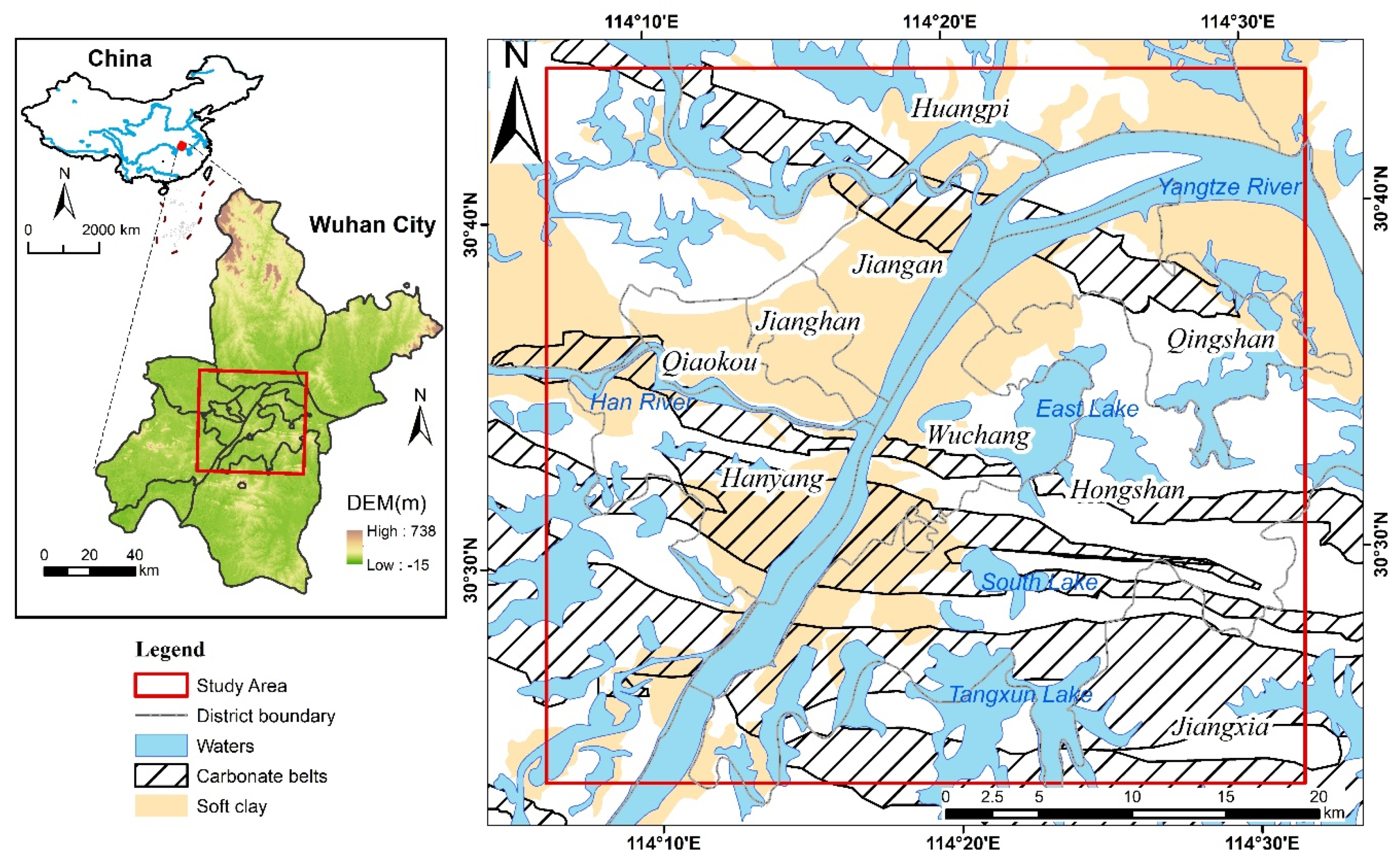
2. Study Area
3. Materials and Methods
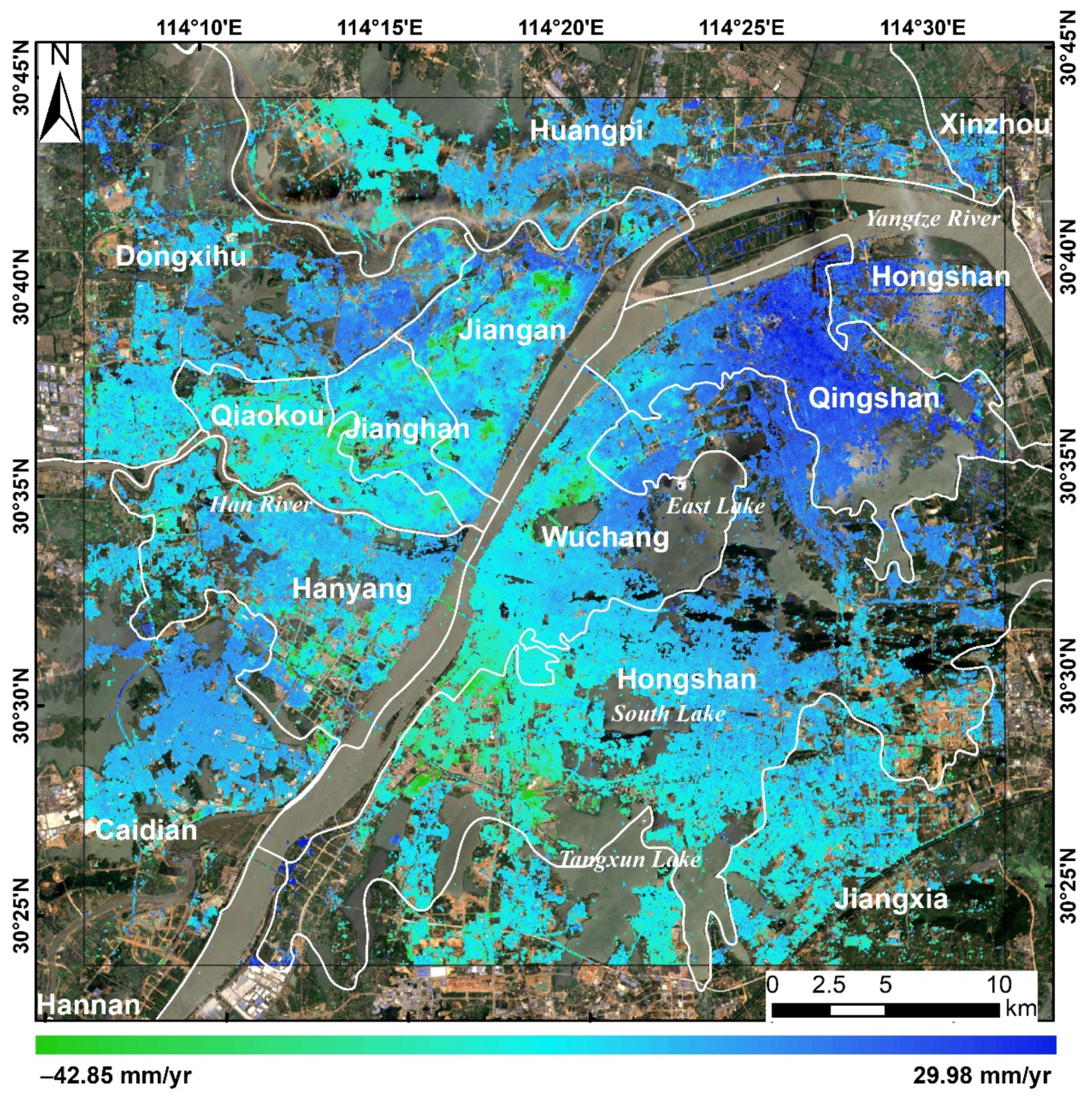
3.1. Land Subsidence Extraction
3.2. Urbanization Metric Quantification
3.3. Exploratory Spatial Data Analysis
3.4. Geographically Weighted Regression Model
4. Results and Discussion
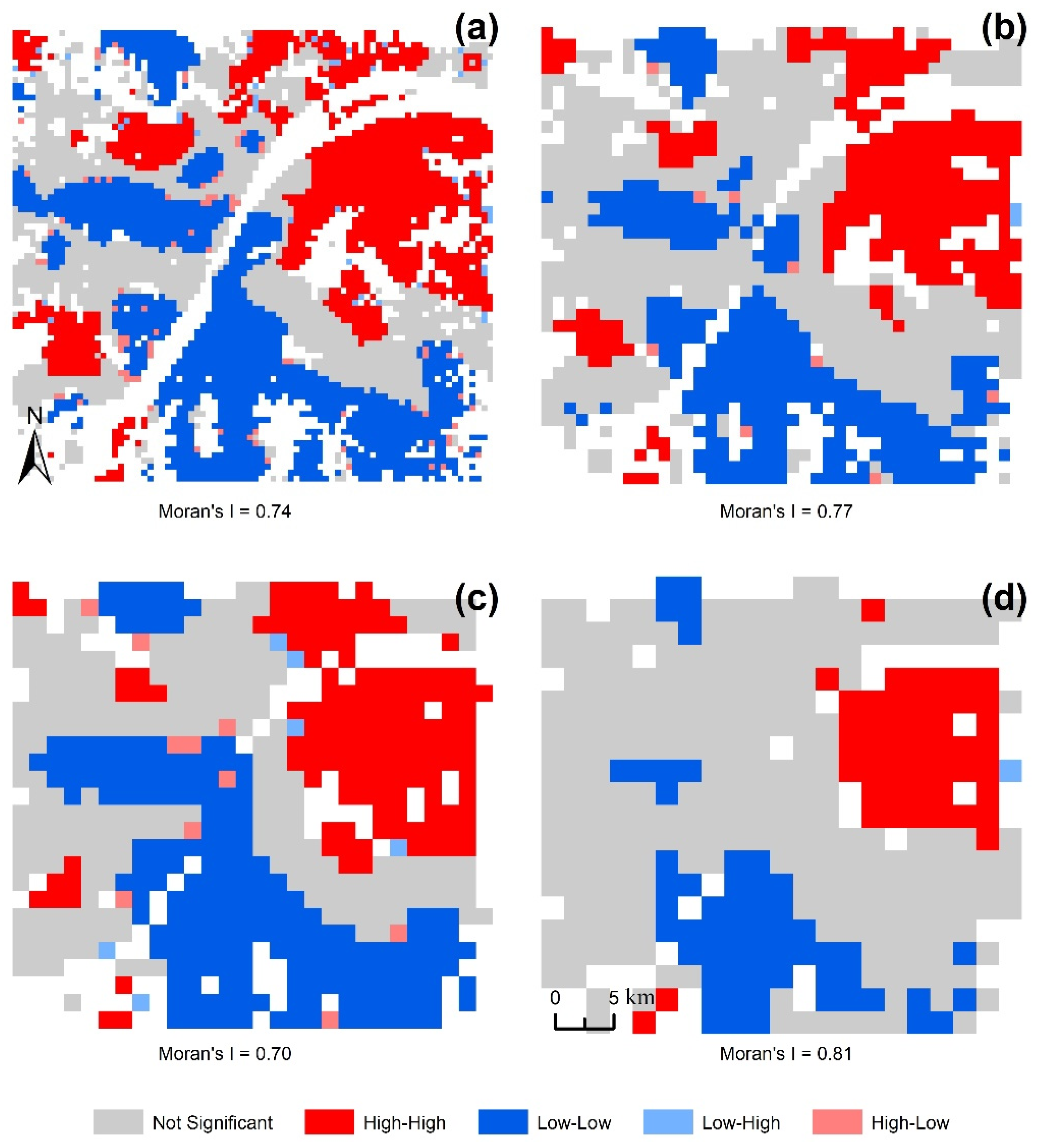
4.1. Spatial Autocorrelations of Land Subsidence
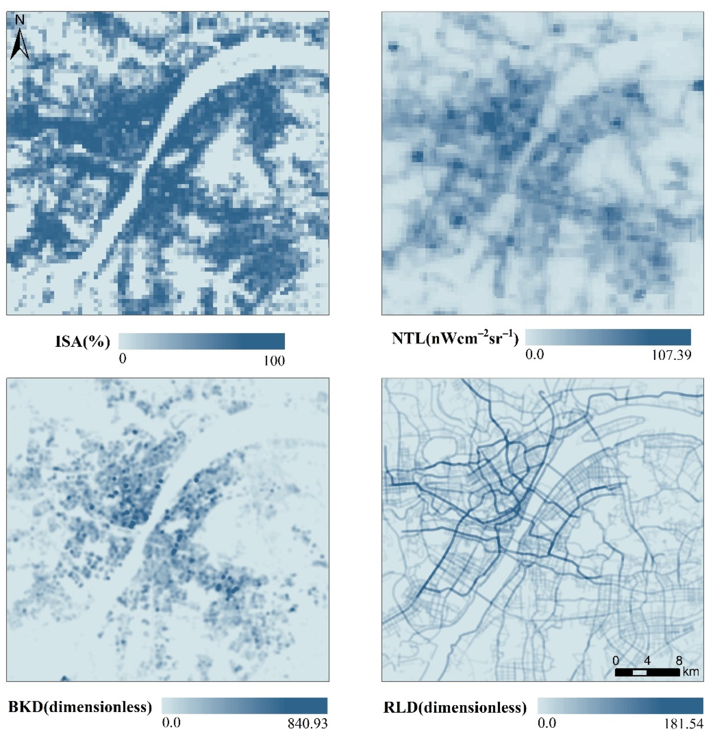
4.2. Spatial Patterns of Urbanization
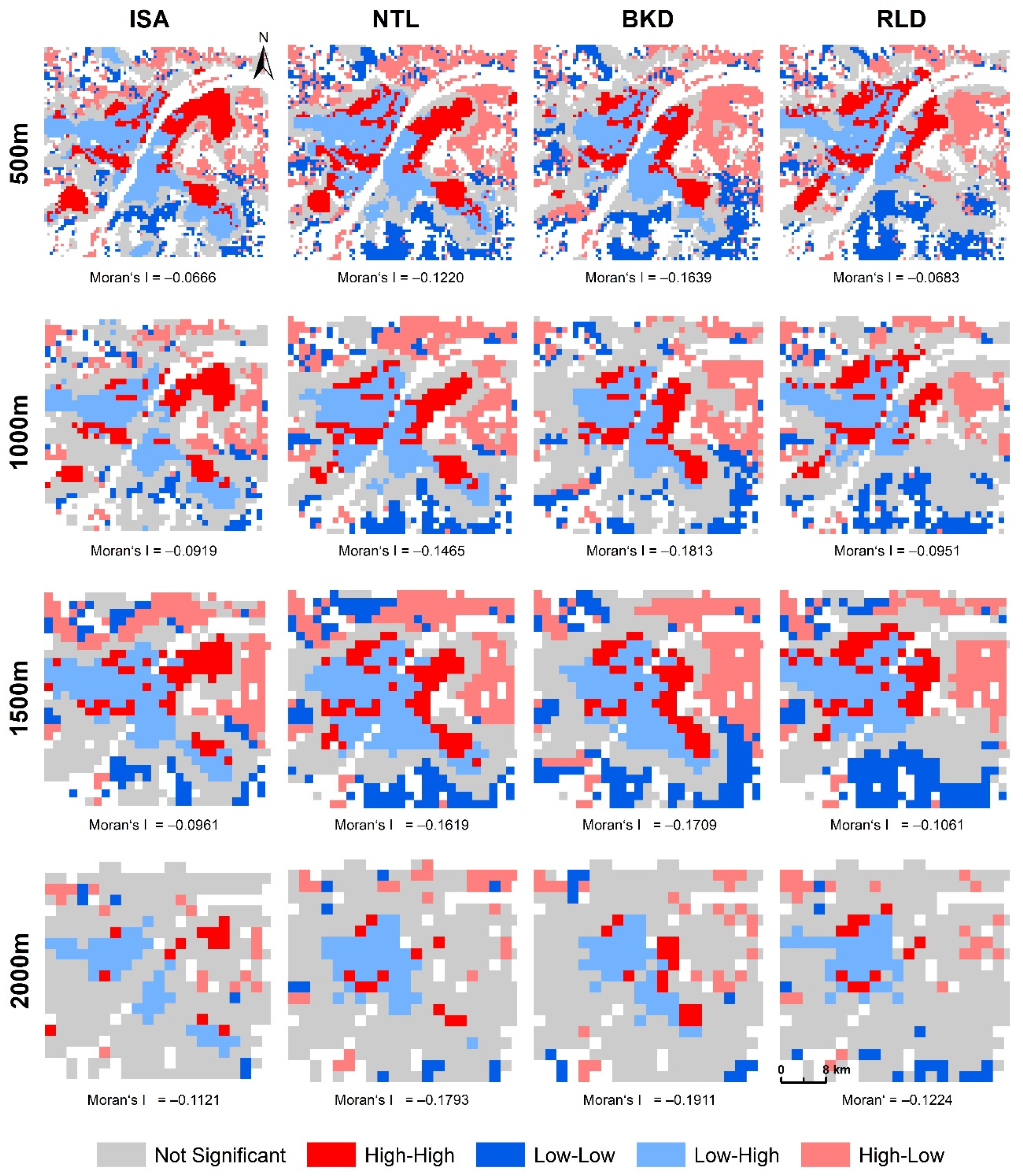
4.3. Spatial Associations between Land Subsidence and Urban Development
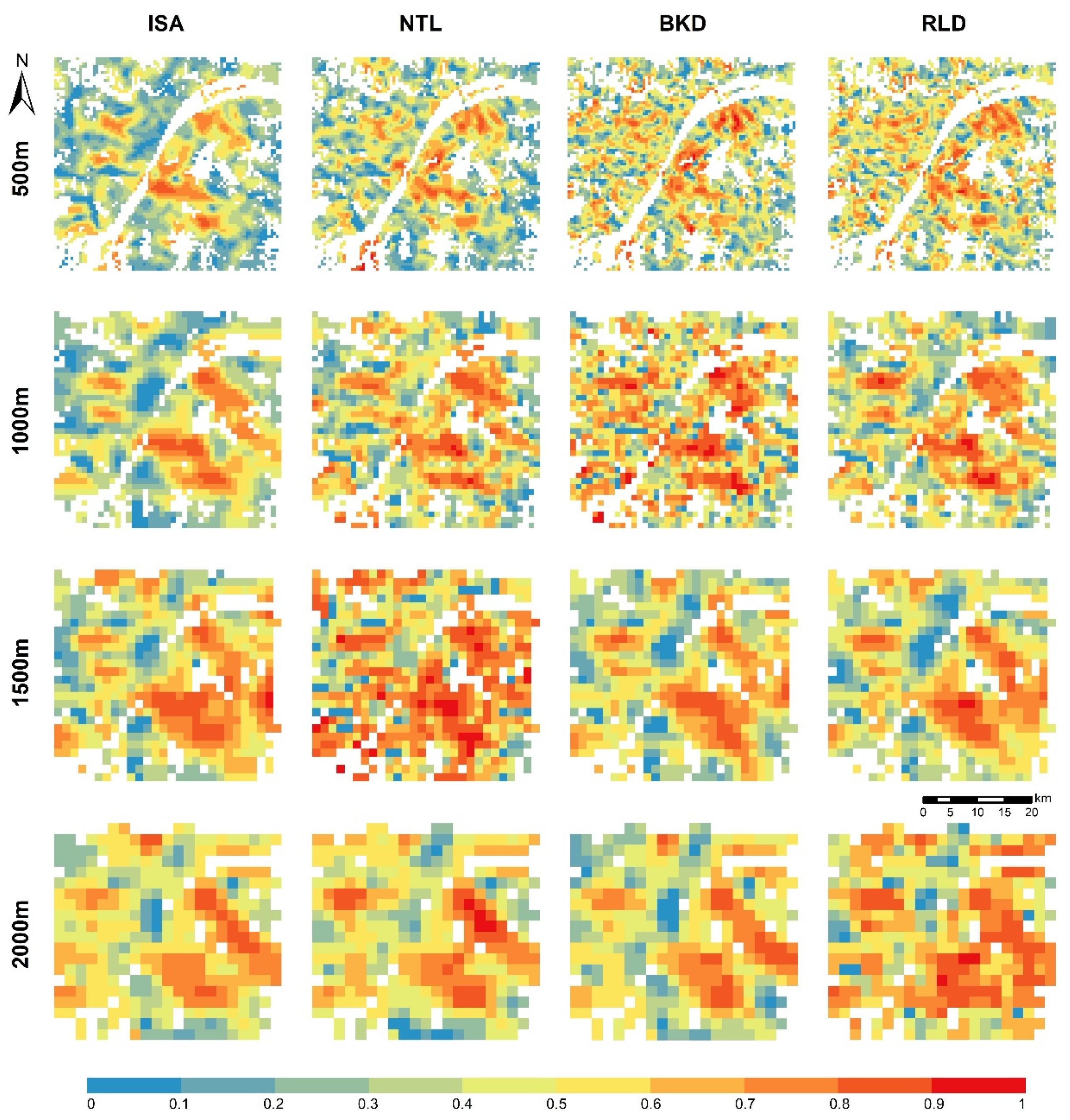
4.4. Impacts of Urbanization on Land Subsidence
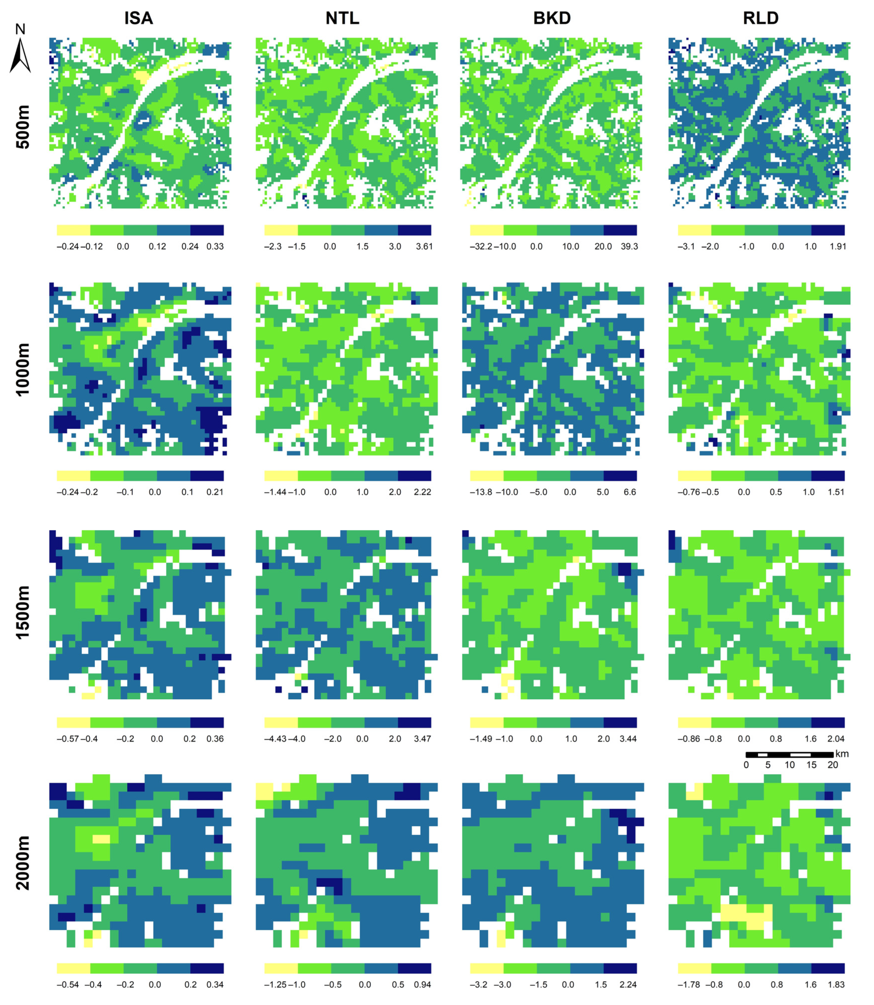
4.5. Scale Effects of Relationships between Land Subsidence and Urbanization
5. Conclusions
Author Contributions
Funding
Data Availability Statement
Acknowledgments
Conflicts of Interest
References
- Chen, F.; Guo, H.; Ma, P.; Lin, H.; Wang, C.; Ishwaran, N.; Hang, P. Radar interferometry offers new insights into threats to the Angkor site. Sci. Adv. 2017, 3, e1601284. [Google Scholar] [CrossRef] [Green Version]
- Zhao, R.; Li, Z.; Feng, G.; Wang, Q.; Hu, J. Monitoring surface deformation over permafrost with an improved SBAS-InSAR algorithm: With emphasis on climatic factors modeling. Remote Sens. Environ. 2016, 184, 276–287. [Google Scholar] [CrossRef]
- Qu, F.; Zhang, Q.; Lu, Z.; Zhao, C.; Yang, C.; Zhang, J. Land subsidence and ground fissures in Xi’an, China 2005–2012 revealed by multi-band InSAR time-series analysis. Remote Sens. Environ. 2014, 155, 366–376. [Google Scholar] [CrossRef]
- Chen, F.; Lin, H.; Li, Z.; Chen, Q.; Zhou, J. Interaction between permafrost and infrastructure along the Qinghai–Tibet Railway detected via jointly analysis of C- and L-band small baseline SAR interferometry. Remote Sens. Environ. 2012, 123, 532–540. [Google Scholar] [CrossRef]
- Chen, W.; Chen, W.; Gong, H.; Chen, B.; Chen, B.; Liu, K.; Gao, M.; Zhou, C. Spatiotemporal evolution of land subsidence around a subway using InSAR time-series and the entropy method. Gisci. Remote Sens. 2017, 54, 78–94. [Google Scholar] [CrossRef]
- Nicholls, R.J.; Lincke, D.; Hinkel, J.; Brown, S.; Vafeidis, A.T.; Meyssignac, B.; Hanson, S.E.; Merkens, J.; Fang, J. A global analysis of subsidence, relative sea-level change and coastal flood exposure. Nat. Clim. Chang. 2021, 11, 338–342. [Google Scholar] [CrossRef]
- Ye, S.; Luo, Y.; Wu, J.; Yan, X.; Wang, H.; Jiao, X.; Teatini, P. Three-dimensional numerical modeling of land subsidence in Shanghai, China. Hydrogeol. J. 2016, 24, 695–709. [Google Scholar] [CrossRef]
- Yu, H.; Gong, H.; Chen, B.; Liu, K.; Gao, M. Analysis of the influence of groundwater on land subsidence in Beijing based on the geographical weighted regression (GWR) model. Sci. Total Environ. 2020, 738, 139405. [Google Scholar] [CrossRef] [PubMed]
- Higgins, S.A. Review: Advances in delta-subsidence research using satellite methods. Hydrogeol. J. 2016, 24, 587–600. [Google Scholar] [CrossRef]
- Ma, P.; Wang, W.; Zhang, B.; Wang, J.; Shi, G.; Huang, G.; Chen, F.; Jiang, L.; Lin, H. Remotely sensing large- and small-scale ground subsidence: A case study of the Guangdong–Hong Kong–Macao Greater Bay Area of China. Remote Sens. Environ. 2019, 232, 111282. [Google Scholar] [CrossRef]
- Zhang, B.; Wang, R.; Deng, Y.; Ma, P.; Lin, H.; Wang, J. Mapping the Yellow River Delta land subsidence with multitemporal SAR interferometry by exploiting both persistent and distributed scatterers. ISPRS J. Photogramm. 2019, 148, 157–173. [Google Scholar] [CrossRef]
- Dinar, A.; Esteban, E.; Calvo, E.; Herrera, G.; Teatini, P.; Tomás, R.; Li, Y.; Ezquerro, P.; Albiac, J. We lose ground: Global assessment of land subsidence impact extent. Sci. Total Environ. 2021, 786, 147415. [Google Scholar] [CrossRef] [PubMed]
- Herrera-García, G.; Ezquerro, P.; Tomás, R.; Béjar-Pizarro, M.; López-Vinielles, J.; Rossi, M.; Mateos, R.M.; Carreón-Freyre, D.; Lambert, J.; Teatini, P.; et al. Mapping the global threat of land subsidence. Science 2021, 371, 34–36. [Google Scholar] [CrossRef]
- Liu, X.; Wang, Y.; Yan, S.; Shao, Y.; Zhou, H.; Li, Y. Ground subsidence characteristics associated with urbanization in East China analyzed with a Sentinel-1A-based InSAR time series approach. Bull. Eng. Geol. Environ. 2019, 78, 4003–4015. [Google Scholar] [CrossRef]
- Ferretti, A.; Prati, C.; Rocca, F. Nonlinear subsidence rate estimation using permanent scatterers in differential SAR interferometry. IEEE Trans. Geosci. Remote Sens. 2000, 38, 2202–2212. [Google Scholar] [CrossRef] [Green Version]
- Ferretti, A.; Prati, C.; Rocca, F. Permanent Scatterers in SAR Interferometry. IEEE Trans. Geosci. Remote Sens. 2001, 39, 8–20. [Google Scholar] [CrossRef]
- Berardino, P.; Fornaro, G.; Lanari, R.; Sansosti, E. A new algorithm for surface deformation monitoring based on small baseline differential SAR interferograms. IEEE Trans. Geosci. Remote Sens. 2002, 40, 2375–2383. [Google Scholar] [CrossRef] [Green Version]
- Usai, S. A least squares database approach for SAR interferometric data. IEEE Trans. Geosci. Remote Sens. 2003, 41, 753–760. [Google Scholar] [CrossRef] [Green Version]
- Heleno, S.I.N.; Oliveira, L.G.S.; Henriques, M.J.; Falcão, A.P.; Lima, J.N.P.; Cooksley, G.; Ferretti, A.; Fonseca, A.M.; Lobo-Ferreira, J.P.; Fonseca, J.F.B.D. Persistent Scatterers Interferometry detects and measures ground subsidence in Lisbon. Remote Sens. Environ. 2011, 115, 2152–2167. [Google Scholar] [CrossRef] [Green Version]
- Liu, Y.; Liu, J.; Xia, X.; Bi, H.; Huang, H.; Ding, R.; Zhao, L. Land subsidence of the Yellow River Delta in China driven by river sediment compaction. Sci. Total Environ. 2021, 750, 142165. [Google Scholar] [CrossRef]
- Meyer, F.J.; McAlpin, D.B.; Gong, W.; Ajadi, O.; Arko, S.; Webley, P.W.; Dehn, J. Integrating SAR and derived products into operational volcano monitoring and decision support systems. ISPRS J. Photogramm. 2015, 100, 106–117. [Google Scholar] [CrossRef]
- Dong, J.; Zhang, L.; Liao, M.; Gong, J. Improved correction of seasonal tropospheric delay in InSAR observations for landslide deformation monitoring. Remote Sens. Environ. 2019, 233, 111370. [Google Scholar] [CrossRef]
- Necsoiu, M.; Onaca, A.; Wigginton, S.; Urdea, P. Rock glacier dynamics in Southern Carpathian Mountains from high-resolution optical and multi-temporal SAR satellite imagery. Remote Sens. Environ. 2016, 177, 21–36. [Google Scholar] [CrossRef] [Green Version]
- Zhang, Z.; Wang, C.; Tang, Y.; Fu, Q.; Zhang, H. Subsidence monitoring in coal area using time-series InSAR combining persistent scatterers and distributed scatterers. Int. J. Appl. Earth Obs. 2015, 39, 49–55. [Google Scholar] [CrossRef]
- Castellazzi, P.; Arroyo-Domínguez, N.; Martel, R.; Calderhead, A.I.; Normand, J.C.L.; Gárfias, J.; Rivera, A. Land subsidence in major cities of Central Mexico: Interpreting InSAR-derived land subsidence mapping with hydrogeological data. Int. J. Appl. Earth Obs. 2016, 47, 102–111. [Google Scholar] [CrossRef]
- Zuo, J.; Gong, H.; Chen, B.; Liu, K.; Zhou, C.; Ke, Y. Time-Series Evolution Patterns of Land Subsidence in the Eastern Beijing Plain, China. Remote Sens. 2019, 11, 539. [Google Scholar] [CrossRef] [Green Version]
- Costantini, M.; Ferretti, A.; Minati, F.; Falco, S.; Trillo, F.; Colombo, D.; Novali, F.; Malvarosa, F.; Mammone, C.; Vecchioli, F.; et al. Analysis of surface deformations over the whole Italian territory by interferometric processing of ERS, Envisat and COSMO-SkyMed radar data. Remote Sens. Environ. 2017, 202, 250–275. [Google Scholar] [CrossRef]
- Zhou, L.; Guo, J.; Hu, J.; Li, J.; Xu, Y.; Pan, Y.; Shi, M. Wuhan Surface Subsidence Analysis in 2015–2016 Based on Sentinel-1A Data by SBAS-InSAR. Remote Sens. 2017, 9, 982. [Google Scholar] [CrossRef] [Green Version]
- Han, Y.; Zou, J.; Lu, Z.; Qu, F.; Kang, Y.; Li, J. Ground Deformation of Wuhan, China, Revealed by Multi-Temporal InSAR Analysis. Remote Sens. 2020, 12, 3788. [Google Scholar] [CrossRef]
- Jiang, H.; Balz, T.; Cigna, F.; Tapete, D. Land Subsidence in Wuhan Revealed Using a Non-Linear PSInSAR Approach with Long Time Series of COSMO-SkyMed SAR Data. Remote Sens. 2021, 13, 1256. [Google Scholar] [CrossRef]
- Bai, L.; Jiang, L.; Wang, H.; Sun, Q. Spatiotemporal Characterization of Land Subsidence and Uplift (2009–2010) over Wuhan in Central China Revealed by TerraSAR-X InSAR Analysis. Remote Sens. 2016, 8, 350. [Google Scholar] [CrossRef] [Green Version]
- Zhang, Y.; Liu, Y.; Jin, M.; Jing, Y.; Liu, Y.; Liu, Y.; Sun, W.; Wei, J.; Chen, Y. Monitoring Land Subsidence in Wuhan City (China) using the SBAS-InSAR Method with Radarsat-2 Imagery Data. Sensors 2019, 19, 743. [Google Scholar] [CrossRef] [Green Version]
- Ding, Q.; Shao, Z.; Huang, X.; Altan, O.; Zhuang, Q.; Hu, B. Monitoring, analyzing and predicting urban surface subsidence: A case study of Wuhan City, China. Int. J. Appl. Earth Obs. 2021, 102, 102422. [Google Scholar] [CrossRef]
- Torres, R.; Snoeij, P.; Geudtner, D.; Bibby, D.; Davidson, M.; Attema, E.; Potin, P.; Rommen, B.; Floury, N.; Brown, M.; et al. GMES Sentinel-1 mission. Remote Sens. Environ. 2012, 120, 9–24. [Google Scholar] [CrossRef]
- Zebker, H.A.; Villasenor, J. Decorrelation in interferometric radar echoes. IEEE Trans. Geosci. Remote Sens. 1992, 30, 950–959. [Google Scholar] [CrossRef] [Green Version]
- Arnold, C.L.; Gibbons, C.J. Impervious surface coverage—The emergence of a key environmental indicator. J. Am. Plan. Assoc. 1996, 62, 243–258. [Google Scholar] [CrossRef]
- Weng, Q. Remote sensing of impervious surfaces in the urban areas: Requirements, methods, and trends. Remote Sens. Environ. 2012, 117, 34–49. [Google Scholar] [CrossRef]
- Gong, P.; Li, X.; Wang, J.; Bai, Y.; Cheng, B.; Hu, T.; Liu, X.; Xu, B.; Yang, J.; Zhang, W.; et al. Annual maps of global artificial impervious area (GAIA) between 1985 and 2018. Remote Sens. Environ. 2020, 236, 111510. [Google Scholar] [CrossRef]
- Zhao, M.; Zhou, Y.; Li, X.; Cheng, W.; Zhou, C.; Ma, T.; Li, M.; Huang, K. Mapping urban dynamics (1992-2018) in Southeast Asia using consistent nighttime light data from DMSP and VIIRS. Remote Sens. Environ. 2020, 248, 111980. [Google Scholar] [CrossRef]
- Chen, Z.; Yu, B.; Yang, C.; Zhou, Y.; Yao, S.; Qian, X.; Wang, C.; Wu, B.; Wu, J. An extended time series (2000–2018) of global NPP-VIIRS-like nighttime light data from a cross-sensor calibration. Earth Syst. Sci. Data 2021, 13, 889–906. [Google Scholar] [CrossRef]
- Cui, Z.; Yang, J.; Yuan, L. Land subsidence caused by the interaction of high-rise buildings in soft soil areas. Nat. Hazards 2015, 79, 1199–1217. [Google Scholar] [CrossRef]
- Tobler, W.R. A Computer Movie Simulating Urban Growth in the Detroit Region. Econ. Geography. 1970, 46 (Suppl. S1), 234–240. [Google Scholar] [CrossRef]
- MORAN, P.A. Notes on continuous stochastic phenomena. Biometrika 1950, 37, 17–23. [Google Scholar] [CrossRef]
- Anselin, L. Local Indicators of Spatial Association:LISA. Geogr. Anal. 1995, 27, 93–115. [Google Scholar] [CrossRef]
- Anselin, L.; Syabri, I.; Kho, Y. GeoDa: An Introduction to Spatial Data Analysis. Geogr. Anal. 2006, 38, 5–22. [Google Scholar] [CrossRef]
- Anselin, L.S.I.S. Visualizing multivariate spatial correlation with dynamically linked windows. In Proceedings of the CSISS Workshop on New Tools for Spatial Data Analysis, Santa Barbara, CA, USA, 10–11 May 2002. [Google Scholar]
- Brunsdon, C.; Fotheringham, S.; Charlton, M. Geographically weighted regressionÐmodelling spatial non-stationarity. Statistician 1998, 47, 432–443. [Google Scholar]
- Brunsdon, C.; Fotheringham, A.S.; Charlton, M.E. Geographically Weighted Regression: A Method for Exploring Spatial Nonstationarity. Geogr. Anal. 1996, 28, 281–298. [Google Scholar] [CrossRef]
- Xiao, R.; Su, S.; Wang, J.; Zhang, Z.; Jiang, D.; Wu, J. Local spatial modeling of paddy soil landscape patterns in response to urbanization across the urban agglomeration around Hangzhou Bay, China. Appl. Geogr. 2013, 39, 158–171. [Google Scholar] [CrossRef]
- Tu, J. Spatially varying relationships between land use and water quality across an urbanization gradient explored by geographically weighted regression. Appl. Geogr. 2011, 31, 376–392. [Google Scholar] [CrossRef]
- Levin, N.; Kyba, C.C.M.; Zhang, Q.; De Sánchez Miguel, A.; Román, M.O.; Li, X.; Portnov, B.A.; Molthan, A.L.; Jechow, A.; Miller, S.D.; et al. Remote sensing of night lights: A review and an outlook for the future. Remote Sens. Environ. 2020, 237, 111443. [Google Scholar] [CrossRef]
- Chen, G.; Zhang, Y.; Zeng, R.; Yang, Z.; Chen, X.; Zhao, F.; Meng, X. Detection of Land Subsidence Associated with Land Creation and Rapid Urbanization in the Chinese Loess Plateau Using Time Series InSAR: A Case Study of Lanzhou New District. Remote Sens. 2018, 10, 270. [Google Scholar] [CrossRef] [Green Version]
- Garreton, M.; Sánchez, R. Identifying an optimal analysis level in multiscalar regionalization: A study case of social distress in Greater Santiago. Comput. Environ. Urban Syst. 2016, 56, 14–24. [Google Scholar] [CrossRef]
- Meentemeyer, V. Geographical perspectives of space, time, and scale. Landsc. Ecol. 1989, 3, 163–173. [Google Scholar] [CrossRef]
- Atkinson, P.M.; Tate, N.J. Spatial Scale Problems and Geostatistical Solutions: A Review. Prof. Geogr. 2000, 52, 607–623. [Google Scholar] [CrossRef]
- Šímová, P.; Gdulová, K. Landscape indices behavior: A review of scale effects. Appl. Geogr. 2012, 34, 385–394. [Google Scholar] [CrossRef]
- Du, S.; Wang, Q.; Guo, L. Spatially varying relationships between land-cover change and driving factors at multiple sampling scales. J. Environ. Manag. 2014, 137, 101–110. [Google Scholar] [CrossRef]
- Luo, X.; Peng, Y. Scale Effects of the Relationships between Urban Heat Islands and Impact Factors Based on a Geographically-Weighted Regression Model. Remote Sens. 2016, 8, 760. [Google Scholar] [CrossRef] [Green Version]
- Zhao, H.; Ren, Z.; Tan, J. The Spatial Patterns of Land Surface Temperature and Its Impact Factors: Spatial Non-Stationarity and Scale Effects Based on a Geographically-Weighted Regression Model. Sustainability 2018, 10, 2242. [Google Scholar] [CrossRef] [Green Version]
- Li, C.; Li, F.; Wu, Z.; Cheng, J. Exploring spatially varying and scale-dependent relationships between soil contamination and landscape patterns using geographically weighted regression. Appl. Geogr. 2017, 82, 101–114. [Google Scholar] [CrossRef]
- Su, S.; Xiao, R.; Zhang, Y. Multi-scale analysis of spatially varying relationships between agricultural landscape patterns and urbanization using geographically weighted regression. Appl. Geogr. 2012, 32, 360–375. [Google Scholar] [CrossRef]


| Scale | ISA | NTL | BKD | RLD |
|---|---|---|---|---|
| 500 m | 0.0570 | −0.0377 | −0.0623 | −0.0581 |
| 1000 m | 0.1267 | −0.0309 | −0.0711 | −0.0038 |
| 1500 m | −0.0281 | −0.0585 | −0.0278 | −0.0129 |
| 2000 m | 0.1150 | 0.1167 | 0.1268 | 0.0216 |
| Scale | Variable | Coefficient | |||||
|---|---|---|---|---|---|---|---|
| Min | Lower Quartile | Mean | Upper Quartile | Max | |||
| 500 m | ISA | −0.2393 | −0.0058 | 0.0240 | 0.0528 | 0.3389 | 0.7525 |
| NTL | −2.2963 | −0.1292 | −0.0026 | 0.1413 | 3.6109 | 0.7929 | |
| BKD | −32.1901 | −0.0593 | 0.0722 | 0.1371 | 39.3492 | 0.8180 | |
| RLD | −3.1004 | −0.0548 | 0.0295 | 0.0913 | 1.9124 | 0.8205 | |
| 1000 m | ISA | −0.2357 | −0.0332 | 0.0126 | 0.0653 | 0.2151 | 0.7535 |
| NTL | −1.4376 | −0.1626 | −0.0126 | 0.1586 | 2.2220 | 0.8191 | |
| BKD | −13.7699 | −0.0816 | 0.0356 | 0.1842 | 6.6497 | 0.8374 | |
| RLD | −0.7648 | −0.0905 | 0.0389 | 0.1339 | 1.5085 | 0.8019 | |
| 1500 m | ISA | −0.5730 | −0.0766 | 0.0043 | 0.1050 | 0.3629 | 0.7895 |
| NTL | −4.4310 | −0.1935 | 0.0129 | 0.2425 | 3.4730 | 0.8667 | |
| BKD | −1.4849 | −0.0952 | 0.1182 | 0.2601 | 3.4356 | 0.7841 | |
| RLD | −0.8631 | −0.1476 | 0.0408 | 0.2192 | 2.0384 | 0.7835 | |
| 2000 m | ISA | −0.5431 | −0.0940 | 0.0013 | 0.1154 | 0.3364 | 0.7701 |
| NTL | −1.2506 | −0.2347 | −0.0581 | 0.1684 | 0.9370 | 0.7805 | |
| BKD | −3.2007 | −0.1089 | 0.0918 | 0.2867 | 2.2430 | 0.7660 | |
| RLD | −1.7809 | −0.2026 | 0.0237 | 0.2558 | 1.8308 | 0.8136 | |
Publisher’s Note: MDPI stays neutral with regard to jurisdictional claims in published maps and institutional affiliations. |
© 2022 by the authors. Licensee MDPI, Basel, Switzerland. This article is an open access article distributed under the terms and conditions of the Creative Commons Attribution (CC BY) license (https://creativecommons.org/licenses/by/4.0/).
Share and Cite
Wang, Z.; Liu, Y.; Zhang, Y.; Liu, Y.; Wang, B.; Zhang, G. Spatially Varying Relationships between Land Subsidence and Urbanization: A Case Study in Wuhan, China. Remote Sens. 2022, 14, 291. https://doi.org/10.3390/rs14020291
Wang Z, Liu Y, Zhang Y, Liu Y, Wang B, Zhang G. Spatially Varying Relationships between Land Subsidence and Urbanization: A Case Study in Wuhan, China. Remote Sensing. 2022; 14(2):291. https://doi.org/10.3390/rs14020291
Chicago/Turabian StyleWang, Zhengyu, Yaolin Liu, Yang Zhang, Yanfang Liu, Baoshun Wang, and Guangxia Zhang. 2022. "Spatially Varying Relationships between Land Subsidence and Urbanization: A Case Study in Wuhan, China" Remote Sensing 14, no. 2: 291. https://doi.org/10.3390/rs14020291
APA StyleWang, Z., Liu, Y., Zhang, Y., Liu, Y., Wang, B., & Zhang, G. (2022). Spatially Varying Relationships between Land Subsidence and Urbanization: A Case Study in Wuhan, China. Remote Sensing, 14(2), 291. https://doi.org/10.3390/rs14020291