Abstract
Urbanization processes greatly change urban landscape patterns and the urban thermal environment. Significant multi-scale correlation exists between the land surface temperature (LST) and landscape pattern. Compared with traditional linear regression methods, the regression model based on random forest has the advantages of higher accuracy and better learning ability, and can remove the linear correlation between regression features. Taking Beijing’s metropolitan area as an example, this paper conducted multi-scale relationship analysis between 3D landscape patterns and LST using Pearson Correlation Coefficient (PCC), Multiple Linear Regression and Random Forest Regression (RFR). The results indicated that LST was relatively high in the central area of Beijing, and decreased from the center to the surrounding areas. The interpretation effect of 3D landscape metrics on LST was more obvious than that of the 2D landscape metrics, and 3D landscape diversity and evenness played more important roles than the other metrics in the change of LST. The multi-scale relationship between LST and the landscape pattern was discovered in the fourth ring road of Beijing, the effect of the extent of change on the landscape pattern is greater than that of the grain size change, and the interpretation effect and correlation of landscape metrics on LST increase with the increase in the rectangle size. Impervious surfaces significantly increased the LST, while the impervious surfaces located at low building areas were more likely to increase LST than those located at tall building areas. It seems that increasing the distance between buildings to improve the rate of energy exchange between urban and rural areas can effectively decrease LST. Vegetation and water can effectively reduce LST, but large, clustered and irregularly shaped patches have a better effect on land surface cooling than small and discrete patches. The Coefficients of Rectangle Variation (CORV) power function fitting results of landscape metrics showed that the optimal rectangle size for studying the relationship between the 3D landscape pattern and LST is about 700 m. Our study is useful for future urban planning and provides references to mitigate the daytime urban heat island (UHI) effect.
1. Introduction
Urbanization has become one of the most important human activities since the 21st century, with people’s living environments requiring continuous improvement [1]. The transformation of natural or semi natural landscapes, such as vegetation, rivers, and cropland, to urban impervious surfaces weakens the surface evapotranspiration and increases the amount of conversion from latent heat to sensible heat, which greatly changes the urban thermal environment and leads to the increase of urban LST [2]. Heat accumulates in urban areas due to urban buildings and human activities, and makes the urban temperature higher than that of surrounding suburbs; this is called an urban heat island (UHI) [3]. In the past decades, researchers have found that factors, including population density, anthropogenic heat release, building distribution, and the 2D and 3D landscape pattern of the city were validated as highly related factors for UHI [4,5,6,7]. The affection of UHI to the urban atmospheric environment, living environment and material circulation usually negatively affects human physical and mental health in urban areas [8,9,10,11]. From 2001 to 2018, China’s newly added urban area accounted for 47.5% of the total, ranking first in the world [12]. As the capital city of China, Beijing has a significant UHI effect, with an average summer heat island intensity of about 2.3–3.4 K [13]. Zhao et al. used the Kriging method with monitoring summer data and proved that high temperatures in the center of Beijing can deteriorate air quality [14]. He et al. demonstrated that synergistic interactions between UHI and heatwaves presents heat-related risks for urban society and residents using observation and a numerical model [15]. Cui et al. indicated that UHI led to the increase of the urban heating and cooling load by statistical analysis of the 50-year 17-station weather data [16]. In summary, high LST in Beijing obviously showed negative effects on living conditions and human health.
Landscape patterns are usually characterized by landscape metrics and spatial statistical methods [17,18,19], and component and spatial configuration are the two major facets delineated by landscape metrics [20]. Traditional 2D landscape metrics depict landscape information in the horizontal projection plane without consideration of the vertical direction [21]. Urban 3D characteristics affect the urban climate and environment in terms of sky visibility, urban canyon air flow, light intensity, and energy accumulation [22,23,24,25], and they also have a significant impact on UHI [26]. The application of 3D landscape metrics can measure the 3D characteristics of the landscape, especially in the urban center with dense buildings and complex vertical landscape structures.
The time scale and spatial scale are the two major scale effects that are considered in landscape ecology [27]. The spatial multi-scale effect in this study included extent and grain sized; the spatial extent was defined by the size of rectangle used to calculated the metrics values at each pixel, and the grain size was defined as the sampling pixel size of the raster image [28]. The spatial heterogeneity of the urban landscape pattern strongly depends on scale. Wu et al.’s analysis of how landscape metrics respond to the change of grain size, extent and direction of the analysis found that the scale effect of landscape metrics could be divided into three kinds, including the predictable response, the more difficult to predict step response and the irregular unpredictable response [27]. Yuan et al. studied the influence of the grain size change on the LST pattern, and discovered the obvious spatial autocorrelation of the distribution of LST and obvious scale correlation of the pattern of LST [29]. These studies mainly consider the 2D characteristics of landscape patterns and ignore the multi-scale dependence between the landscape pattern and UHI in 3D space.
The main methods to study the multi-scale relationship between LST and urban landscape patterns include linear regression, geographically weighted regression, the multi-parameter method, and spatial analysis, etc. [30,31]. Huang et al. [32] and Gage et al. [33] both studied the relationship between LST (retrieved by Landsat 8 images) and urban 3D characteristics; Lai et al. proved that building height, sky view factor and building density significantly effect LST (retrieved by Landsat 8 and Landsat 5 images) [34]. Guo et al. analyzed the effect of 3D building configuration on diurnal and nocturnal LST (retrieved by Landsat 8 and ASTER images) [35]. However, most of these methods are based on linear models that describe the correlation between multiple pattern independent variables and LST by the process of regression. Correlations usually exist among different independent variables in the process of regression, which inevitably causes over-fitting of the regression model. A machine learning-based regression model trains the model using the same data of regression, and analyzes and predicts the relationship between the landscape pattern and LST by the trained model [36]. Compared with the traditional linear regression model, the machine learning regression model, based on the tree model, has the advantages of higher accuracy, better learning ability and strong generalization ability, which can better describe the nonlinear relationship between the pattern and LST, and can remove the multicollinearity problem between landscape metrics in the regression process. Yu et al. used an extreme gradient boosting tree (XGBR) model and the Sharpley Additive Explained (SHAP) method to study the relationship between 3D landscape patterns and LST in Shanghai, and obtained information on the effect of different building heights on LST and the mitigation effect of vegetation on UHI [37]. Cristobal Pais et al. constructed a deep fire framework based on convolutional neural network (CNN) and conducted landscape topology analysis in southeastern Chile, proving that topological relations among different land types are the key cause of wildfires [38]. Lin et al. analyzed the influence of a 3D building structure on emissions based on random forest regression, and found that the building coverage rate, average building number and space crowding degree are the main factors affecting changes in emissions, and that emissions are positively proportional to building density and population density [39]. Most of the above studies were conducted on a single scale, and lack the analysis of multi scale dependence between landscape patterns and LST.
Taking Beijing’s metropolitan area as an example, this article combined 3D landscape metrics with the regression model of machine learning, to study 3D multi-scale effects between the landscape pattern and UHI. The concrete content includes: (1) establishing the regression model of landscape metrics and LST based on random forest regression to compare the response effects of 2D and 3D landscape metrics on LST; (2) explore the response of landscape metrics to LST at different grain sizes and extents in order to determine the multi-scale relationship between the LST and landscape pattern. Our results can provide reference for urban planning and construction in decreasing LST.
2. Materials and Methods
2.1. Study Area
Beijing is located at 115.7°–117.4°E and 39.4°–41.6°N, with an area of 16,410.54 (Figure 1). Beijing is the political, cultural, scientific and technological, and innovation center of China [40]. The spatial pattern of Beijing takes the old city as the center and gradually expands outward, showing a concentric circle development pattern. We chose the inner region of the fourth ring road and the second ring road as our two research areas. The total area within the second ring road is about 62 , and this is the old city. Buildings in the center part along the south to north of this region are mainly traditional dwellings with courtyards, with a lower building height and higher density, and higher buildings are mainly distributed along Chang’an Street and the second ring road. The fourth ring road covers an area of approximately 302 and is comprised of a highly built-up urban landscape.
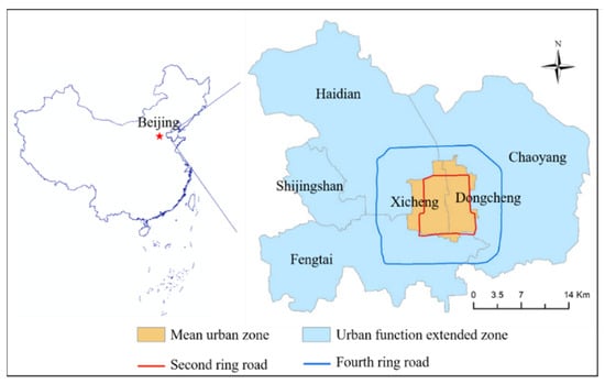
Figure 1.
Study area.
2.2. Data and Preprocessing
We gave radiative calibration and atmospheric correction to the Landsat 8 OLI (Operational Land Imager) and TIRS (Thermal Infrared Sensor) Level-1 (Landsat 8) image, which was used to retrieve LST. Landsat 8 is the eighth satellite in the U.S. Landsat program. It was developed by National Aeronautics and Space Administration (NASA) in collaboration with the United States Geological Survey (USGS) and built by Orbital Science Corporation. Since the UHI effect of summertime testified more significantly than other seasons [41], we chose an image which was taken on 14 June 2019 at 02:53:04 (Greenwich Mean Time) which was the most suitable image in the summer of 2019 with sunny weather and no clouds in our research area. The image has a spatial resolution of 30 m and the land cloud cover of 1.42%. The atmosphere temperature on 14 June 2019 was between 308.2 K and 293.2 K, and it was about 304.6 K at the time of image acquisition with relative humidity of 24%.
Land cover data (forest, grassland, water and impervious surface) with 10 m resolution was downloaded from Finer Resolution Observation and Monitoring-Global Land Cover (FROM-GLC10) data set (http://data.ess.tsinghua.edu.cn/ accessed on 12 April 2020), which was produced from the Landsat Thematic Mapper (TM) and Enhanced Thematic Mapper Plus (ETM+). The building height data was obtained from Baidu, Inc. with a resolution of 3 m.
We defined 10 m and 30 m two grain sizes in order to study the scale effect on LST and the landscape pattern. We resampled 30 m LST into 10 m resolution by the cubic convolution method, resampled 10 m land cover data and 3 m building height data into 30 m by the nearest neighbor method. All the data (Figure 2) and preprocessing were completed under the WGS1984 coordinate system and UTM projection.
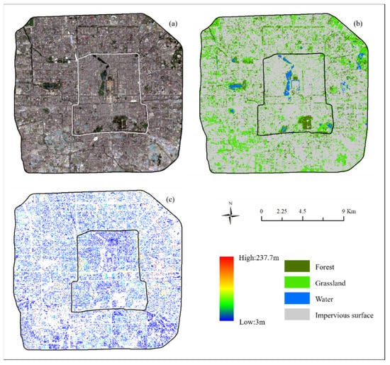
Figure 2.
Landsat 8 image, land cover map and building height of two study areas. (a) Landsat 8 image; (b) land cover map; (c) building height.
2.3. Method
As Figure 3 shows, our research comprises the following steps: (1) LST was retrieved from Landsat 8 image using the mono-window algorithm; (2) 2D/3D landscape metrics were calculated using land cover data and building height data; (3) the PCC was calculated between LST and 2D/3D landscape metrics; (4) multiple linear regression and RFR were used to analyze the multi-scale relationship between the LST and 2D/3D landscape pattern; (5) the Coefficients of Rectangle Variation (CORV) was introduced to obtain the optimal calculation rectangle size in analyzing the 3D landscape pattern in the fourth ring road of Beijing.
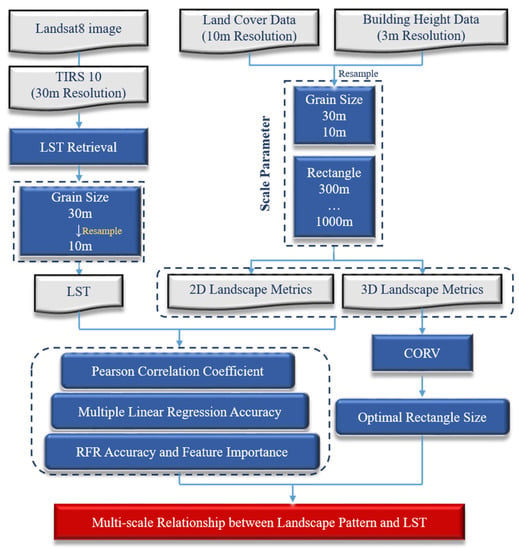
Figure 3.
Flow chart of the whole research.
2.3.1. Land Surface Temperature Retrieval
LST of the study area was retrieved by thermal infrared band 10 (TIRS10) using the mono-window algorithm [42,43] after radiometric calibration and atmospheric correction. The TIRS10 band can be converted to brightness temperature using the following Equation [44]:
where is the brightness temperature of TIRS10, is the adjusted factor of TIRS10, is the digital number of Landsat 8 image, is the tuning parameter of TIRS10, , and [30]. Finally, LST can be obtained by Equation (2):
where is the land surface emissivity calculated according to the normalized difference vegetation index (NDVI) [45], τ is atmospheric transmissivity, and are the atmospheric upward radiation intensity and atmospheric downward radiation intensity, respectively, obtained by the official website of Meteomanz (http://www.meteomanz.com/ accessed on 6 November 2019) and Atmospheric Correction Parameter Calculator (https://atmcorr.gsfc.nasa.gov/ accessed on 6 November 2019).
2.3.2. Landscape Metrics
Landscape metrics measure landscape patterns by describing characteristics of the component and spatial configuration of different patches [20]. In this paper, component metrics, configuration metrics and roughness metrics were calculated respectively at different scales [17]. The component metrics generally describe the land cover types and relative abundance of various types within the landscape, while the configuration metrics focused on the spatial location, distribution characteristics and spatial relations of different types of landscape pixels or patches [20]. Roughness metrics as 3D landscape metrics are generally used to describe the surface features of landscapes. In this paper, roughness metrics are used to quantify the spatial form and undulation characteristics of urban buildings. We read relative articles and sorted some commonly used landscape metrics for quantitative description of the landscape pattern in our study [21,32,46,47,48,49]. The detailed description of all metrics used in this article is given in Table 1.

Table 1.
Landscape metrics used in this paper and their ecological significances.
2.3.3. Pearson Correlation Coefficient
PCC can evaluate the linear correlation between two variables with a value between −1 and 1 [50,51,52] which can be calculated by Equation (5):
where represented LST, represented 2D/3D landscape metrics. When the two variables are distributed on a straight line, PCC is equal to 1 or −1; when there is no linear relationship between the two, the value of PCC is 0.
2.3.4. Multiple Linear Regression
Regression analysis is a statistical process used to evaluate the relationship between variables and explain the relationship between independent and dependent variables. The linear regression model is one of the regression analysis methods [53]. When the number of independent variables evaluated is greater than 1, it is called multiple linear regression. In our research, it was used at first to evaluate the relationship between LST and landscape pattern as a comparison for random forest regression. The fitting image of multiple linear regression is a straight line, and the highest degree of each independent variable is 1. The multivariate linear relationship between the dependent variable (LST) and independent variable (landscape metrics) can be calculated as follows:
where is the parameter of each 2D/3D landscape metrics in regression, is the constant parameter, and is the number of metrics.
2.3.5. Random Forest Regression
Random forest is a bagging ensemble machine learning algorithm [54], which is mainly applied in classification and regression. It has been widely used in economics, statistics, the medical field, environmental studies and many other fields [55,56,57,58]. One of the advantages of the tree model is that it can remove the multicollinearity between independent variables in the regression process. It also has a strong ability to learn data sets, and so is suitable for the regression task with a large sample [59]. Random forest regression (RFR) is a kind of integration algorithm based on a regression tree model [54]. Compared with a traditional linear regression model, RFR has higher accuracy with the same data set and can handle higher dimensional feature sets because of its low sensitivity to the outliers in the data set with a lower risk of over fitting, especially for the absence of some characteristics in the data set [60]. The RFR algorithm establishes several parallel regression trees during regression and obtains the regression accuracy of each parallel tree, and the regression accuracy of the whole forest is given by the average accuracy of all regression trees (Figure 4). In this study, surface temperature was used as a label, and different landscape metrics (15) were used as regression features. The results on each scale in the two study areas were made into 16 columns and several rows (sample number) of data sets which were input into the RFR model for regression. The training set used 70% of the randomly established tree model, and the remaining 30% was used as the test set to test the regression accuracy of the model. Finally, the RFR accuracy of the landscape metrics and LST at various scales in the two study areas were obtained with the feature importance of each metric.

Figure 4.
Flow chart of random forest regression.
The RFR model calculates the contribution of different metrics in the regression process based on the Gini coefficient, which can be obtained from the following formula [54]:
where is the number of metrics, is the sample weight of metric , and the importance of metric on node m is the variation of the Gini coefficient before and after the node m branches:
where and are the Gini coefficients of the two new nodes after branching, respectively. If the nodes of metric appear in regression tree and is in set , the variable importance measure (VIM) of in this tree is:
If there are n trees in the random forest, then:
Finally, all obtained importance scores are normalized as:
where is the Gini coefficient of metric j, is the sum of the information gain of all metrics.
2.3.6. Coefficient of Rectangle Variation
The metrics at each pixel were calculated in a rectangular area to analyze the distribution of component and configuration characteristics [61,62]. The size of the rectangular area was usually manually selected by the sensitivity to calculate the value of the metrics centered at each pixel of the study area [63], which may generally affect the results of the landscape pattern. When the rectangles are too small, the local characteristics of the landscape will be stronger than the overall characteristics, and it is difficult to obtain the general landscape pattern information within the whole range. If the rectangles are too large, the resolution of the result will be reduced, and the local landscape pattern information inside the rectangle will be lost. In order to obtain the optimal calculation rectangle size suitable for studying the multi-scale relationship between LST and 3D landscape pattern, the Coefficients of Rectangle Variation (CORV) is introduced in this paper, which can be obtained from the following formula:
where is the total number of pixels in a rectangle, is the metrics value of rectangle , and is the average metrics value of rectangle . CORV reflects the changes in the law of the metrics in a different rectangle. The larger the value is, the greater the difference of the metrics in different rectangles is, and a single rectangle tends to reflect the local information of the landscape. The smaller the value is, the smaller the change of the metrics is at the rectangle size, and the more it can reflect the overall landscape pattern of the study area.
3. Results
3.1. LST Distribution in the Second and the Fourth Ring Road of Beijing
We classified LST into three levels: high temperature (318–330.6 K), medium temperature (312.8–318 K) and low temperature (296.2–312.8 K) by natural discontinuity point classification. Figure 5 shows LST distribution in the study area and the proportion of land types at different levels of LST. It can be seen that LST in Beijing was relatively high in summer; the highest, average, and lowest temperature in the fourth ring road and the second ring road were 330 K, 316.8 K, and 269.1 K and 330.6 K, 317.3 K, and 296.1 K, respectively. The proportion of grassland in the medium temperature decreased from 10.06% to 7.57%, and in the low temperature decreased from 5.88% to 2.76%. The proportion of water in the whole research area is small, but during the low temperature the water increased from 1.05% to 2.47%. The proportion of impervious water surface at this time was the highest in the research area, up to 75%. The overall proportion of impervious water surface in the fourth ring road is less than that of the second ring road, but in the middle and the low temperatures, there was the opposite result, and the proportion of the low temperature decreased from 3.24% to 1.45%. The proportion of the medium temperature region decreased from 32.63% to 30.42%, and during the high temperatures the region increased from 36.86% to 44.21%. The results indicate that, in the area within the second ring road, the impervious surface positively contributed to the LST more significantly than it did in the area within the fourth ring road. In addition, it can also be seen from the LST distribution figure that the LST on the edge of the fourth ring road—especially in the northern margin region—is relatively low, and the overall surface temperature has a decreasing trend from the center to the periphery. The maximum temperature of the area within the second ring road was lower than that of the area in the fourth ring road, while the average temperature was slightly higher than that of the fourth ring road. There was an obvious high temperature gathering area in the middle of the second ring road, as well as in the north, except for in the water area.
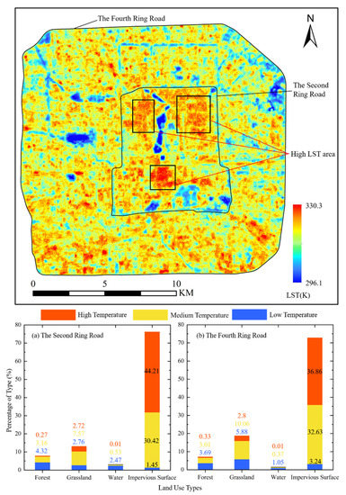
Figure 5.
The distribution of LST and the proportion of land types at different temperature levels in the study area. (a) the second ring road; (b) the fourth ring road.
3.2. Pearson Correlation Coefficient between Landscape Metrics and LST
3.2.1. Pearson Correlation Coefficient between Landscape Metrics and LST at 10 m Grain Size
Figure 6 shows the PCC between the LST and 2D/3D landscape metrics at the 10 m grain size. All of the results were calculated under the significance of 0.05. In general, the correlation between the 3D landscape metrics and LST is generally higher than that of the 2D. Among the three types of metrics, the correlation between the configuration metrics and LST is the highest, the correlation between the component metrics and LST is the second highest, and the correlation between the roughness metrics and LST is the weakest. These results indicate that both in 2D and 3D landscapes, the proportion and configuration of different land types are the most important factors affecting LST. Among the 15 metrics, SHDI and SHEI had the highest correlation with LST. In terms of 3D landscape metrics, the composition metrics and configuration metrics in the second ring road and the fourth ring road were the same. Among the component metrics, LPI, MESH and COHESION were positively correlated with LST, and ED and NP were negatively correlated with LST. LPI and COHESION had a strong correlation with LST, while MESH was the weakest. The results showed that the increasing proportion of the dominant land type (impervious surface) in the study area would lead to the increase of LST. All five configuration metrics were negatively correlated with LST, in which SHDI and SHEI have the strongest correlation with LST, and LSI has the weakest correlation with LST. The correlation between the component metrics and configuration metrics and LST increases with the increase of rectangular size. When the size increased to 700 m or so, the increase rate slowed down and tended to be stable.
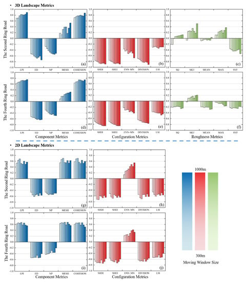
Figure 6.
PCC between LST and landscape metrics at 10 m grain size. (a–f) PCC between LST and 3D landscape metrics at 10 m grain size; (g–j) PCC between LST and 2D landscape metrics at 10 m grain size.
The correlation between roughness metrics and the LST was relatively weak, and there are some differences between the results in two study areas. Within the second ring road, the SQ, SKU and MAX were positively correlated with LST, the MEAN and SVF were negatively correlated with LST, and SVF showed the strongest correlation. In the fourth ring road, SQ, MEAN, MAX and SVF were negatively correlated with LST, while SKU was positively correlated with LST. The mean height of the rectangle decrease refers to the reduction in the number of buildings and building density. The results showed that increasing the height and decreasing the density of urban buildings can decrease the daytime LST. This result is similar to those of previous studies: in daytime, urban planning should meet the daylight standard, which means that the distance between buildings generally increases with the building height [34]. High density traditional dwellings and courtyards with a low height have almost the highest LST and the largest high temperature aggregation of the whole study area (Figure 5). For the regions between the fourth ring road and the second ring road, the higher LST were mainly distributed in the south area with high height and density residential land, which was relatively cooler compared to the lower buildings in the second ring road. The correlation between the roughness metrics and LST was greatly affected by the rectangle variation, and the correlation between SVF and LST was higher in the second ring road.
The correlation between the 2D landscape metrics and LST was similar to that of 3D landscape metrics, except for ENN-MN. The correlation between ENN-MN and LST was positively in the 2D surface, and negatively in the 3D space, which can be attributed to the giant distance value difference between the mean of the minimum patch distance in the 2D space and 3D space. This was because when calculating the nearest Euclidean distance of the building patches, the value of the fluctuation of the 3D surface was much larger than that of the 2D surface, which played a dominant role in calculating the average ENN of the four land types. The positive correlation between ENN-MN and LST in 2D indicated that the more dispersed the vegetation and water patches were, the worse the cooling effect was, while the negative correlation between the ENN-MN and LST in 3D indicated that the LST increased with the accumulation of impervious surfaces.
3.2.2. Pearson Correlation Coefficient between Landscape Metrics and LST at 30 m Grain Size
The PCC of 30 m grain-size landscape metrics and LST (Figure 7) were highly consistent with the 10 m grain-size results. The correlation of the metrics of 30 m grain size was slightly lower than that of the 10 m grain size, and the correlation between component and configuration metrics and LST was high, while the correlation between roughness metrics and LST was low. The correlation between the 3D landscape metrics and LST increased with the increase of rectangle size, and tended to be stable when the rectangle size reached 700 m. In general, the change of grain size showed little effect on the overall landscape pattern in the study area, while the improvement of the resolution could improve the correlation between the landscape metrics and LST.
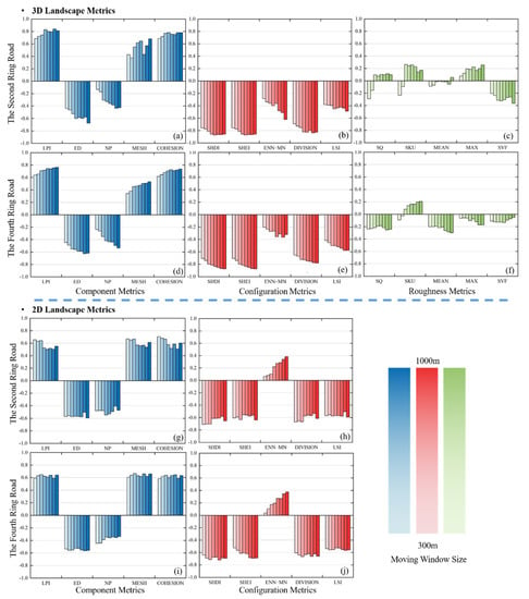
Figure 7.
PCC between LST and landscape metrics at 30 m grain size. (a–f) PCC between LST and 3D landscape metrics at 30 m grain size; (g–j) PCC between LST and 2D landscape metrics at 30 m grain size.
3.3. Multiple Linear Regression between Landscape Metrics and LST
3.3.1. Multiple Linear Regression between Landscape Metrics and LST at 10 m Grain Size
In this paper, the data set made at the initial stage of the experiment was first input into the multiple linear regression model to compare with the RFR model. The results showed that the interpretation effect of the 3D landscape metrics on LST was better than that of the 2D landscape metrics in both study areas from the view of regression accuracy (Figure 8) which was already proved by some previous studies [21,37]. The linear regression accuracy between 3D metrics and LST increased steadily with the increase of rectangle size, and the increase slowed down when the rectangle size reached 700 m. The linear regression accuracy in the second ring road is higher than that in the fourth ring road. The linear regression accuracy of the 3D landscape metrics and LST in the second ring road increased from 0.76 to 0.90, and in the fourth ring road increased from 0.63 to 0.83. The accuracy of the linear regression between the 2D landscape metrics and LST fluctuated and decreased with the increase of the rectangle size. The multiple linear regression accuracy of the 2D landscape metrics and LST decreased from 0.60 to 0.41 in the second ring road, and from 0.58 to 0.40 in the fourth ring road. In addition, the multiple linear regression accuracy was higher in the second ring road. This is because the proportion of impervious surfaces of the second ring road is higher than that of the fourth ring road, which means more buildings (3D landscape features) in the area which make the value differences more significant between the 3D and 2D landscape metrics.
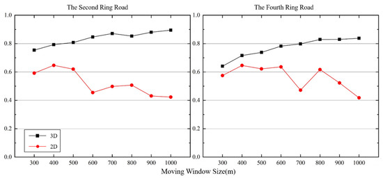
Figure 8.
The of the multiple linear regression model between LST and landscape metrics at 10 m grain size.
3.3.2. Multiple Linear Regression between Landscape Metrics and LST at 30 m Grain Size
The linear regression accuracy of landscape metrics and LST at 30 m grain size (Figure 9) is also very similar to that of the 10 m grain size. The accuracy of the 3D landscape metrics and LST linear regression increases with the increase of the rectangle size, while the accuracy of the 2D landscape metrics and LST decreased with the increase of the rectangle size, and the accuracy of the second ring road was slightly higher than that of the fourth ring road. The linear regression accuracy of 3D in the second ring area increased from 0.72 to 0.85, and in the fourth ring road increased from 0.60 to 0.83. This phenomenon was similar to the results obtained in Section 3.2.2, indicating that, although the change of research granularity cannot change the overall landscape pattern of the study area, it can describe the landscape pattern of the study area more accurately.
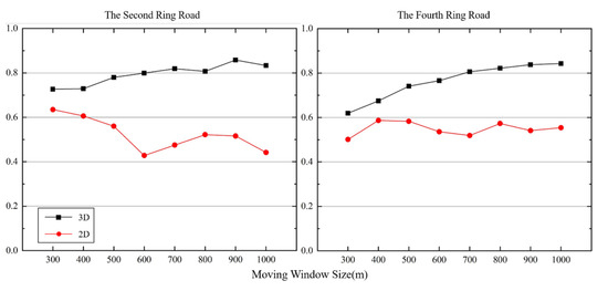
Figure 9.
The of the multiple linear regression model between LST and landscape metrics at 30 m grain size.
3.4. Random Forest Regression between Landscape Metrics and LST
The of the RFR model between the landscape metrics and LST (Figure 10) were similar to the multiple linear regression results. The RFR accuracy between the 3D landscape metrics and LST was still higher than that of the 2D metrics, and the 3D accuracy showed an upward trend with the increase of the rectangle size, while the 2D accuracy shows a downward trend. At the 10 m grain size, the of the RFR model between the 3D landscape metrics and LST increased from 0.81 to 0.93 in the second ring road, and 0.70 to 0.80 in the fourth ring road. The of the RFR model of the 2D landscape metrics and LST in the second ring road decreased from 0.70 to 0.02, and from 0.6 to 0.1 in the fourth ring road. At the 30 m grain size, the of the RFR model between the 3D landscape metrics and LST in the second ring road increased from 0.78 to 0.82, and increased from 0.68 to 0.80 in the fourth ring road. The of the RFR model of the 2D landscape metrics and LST in the second ring road decreased from 0.72 to 0.04, and in the fourth ring road decreased from 0.58 to 0.45. In addition, the RFR regression accuracy at the small rectangle size (300–600 m) was generally higher than the multiple linear regression accuracy, while the RFR regression at a large rectangle (700–1000 m) showed slightly lower accuracy. Compared with the RFR results of the second ring road, the RFR accuracy of the fourth ring road was significantly more stable, which was related to the number of samples involved in the regression. The 30 m grain size with the 300 m rectangle size in the fourth ring road has the largest data set, which contains 3219 samples, and the 1000 m rectangle size in the second ring road has the smallest data set, which contains 44 samples. This indicates that the RFR results were better than the multiple linear regression in the case of large sample sizes. Logan et al. used seven different models to regress a large sample of multiple variables and LST, and the results also showed that the accuracy of RFR was higher than that of the linear model [64]. The regression between the 2D landscape metrics and LST showed a weak interpretation of the 2D landscape metrics on LST. At the same time, a poor learning effect existed in RFR on small data sets due to the small number of calculated results in a large rectangle, resulting in extremely low regression accuracy of RFR when the rectangle size was 1000 m.
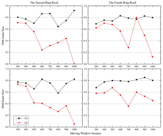
Figure 10.
The of the RFR model between LST and landscape metrics.
Figure 11 shows the feature importance of different metrics in RFR; the metrics in each row are ranked by the sum of the contribution of different rectangle sizes. The result of the landscape metrics’ contribution was similar to that of PCC, which meant that the metrics with higher contribution in the regression have a higher correlation coefficient. Overall, SHDI and SHEI had the highest feature importance and NP had the lowest. Among the three types of landscape metrics, the importance of configuration metrics was the highest. The importance of roughness metrics in the fourth ring road was higher than that of the component metrics, and the importance of the second ring road had an opposite result. The contribution of the five metrics, except NP, decreased with the increase of the rectangle size, and the sensitivity of the component metrics to the rectangle size in the 30 m grain size was lower than that in the 10 m grain size. Except SHDI and SHEI, the importance of configuration metrics was slightly lower at all scales. Roughness metrics had a high importance in the fourth ring road, and the importance decreased with the increase of rectangle size. In the second ring road, the importance of the component metrics, such as MESH, LPI and COHESION, was relatively high. The importance of MESH, LPI, COHESION and NP in the 30 m grain size increased with the increase of the rectangle size. The roughness metrics MEAN and SVF were of high importance, and their importance decreased with the increase of the rectangle size. The regularity of feature importance is not strong at the 10 m grain size, but the results still conform to the overall law of this study: SHEI and SHDI have the highest contribution, and this is also very close to the calculation results of the 30 m grain size in the second ring road area.
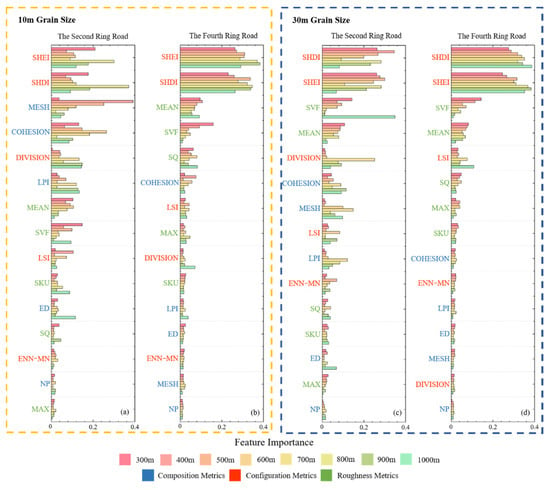
Figure 11.
Feature importance of 3D landscape metrics to LST in RFR. (a,b) are the feature importance of each metrics at 10 m grain size; (c,d) are the feature importance of each metrics at 30 m grain size.
3.5. The CORV of 3D Landscape Metrics
3.5.1. The CORV of 3D Landscape Metrics at 10 m Grain Size
The CORV of different 3D landscape metrics fitted by the power function obtained the optimal rectangle size for analyzing the relationship between LST and the 3D landscape pattern. The results of each metric varied at a great magnitude, and normalization was conducted before the fitting to homogenize the CORV of metrics with significant differences. Figure 12 shows the CORV of each 3D landscape metric at the 10 m grain size. The abscissa is the size of different rectangles (m), and the of each power function fitting is displayed below each figure. It can be seen that the fitting accuracy of the CORV of most metrics was high, and the CORV decreased with the increase of the rectangle size. The CORV decreased rapidly when the rectangle size was between 300 m to 500 m. They approached the minimum value and tended to be stable when the rectangle size reached 700 m. Among the 15 metrics in the second ring road, the of the CORV power function fitting of nine metrics, such as COHESION, was higher than 0.8; the fitting of DIVISION was between 0.6–0.8 (0.66); and the fitting of the remaining five landscape metrics, such as LPI and ED, was less than 0.3. The fitting accuracy of CORV in the fourth ring road was lower than that in the second ring road. The fitting of MESH and COHESION was higher than 0.8, the LPI and MEAN was between 0.6–0.8, the SHDI and other three metrics were between 0.4–0.6, and the ED and other four metrics were less than 0.3.
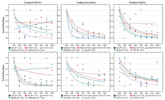
Figure 12.
Power fitting of the normalized CORV of each 3D landscape metrics at the 10 m grain size.
3.5.2. The CORV of 3D Landscape Metrics at 30 m Grain Size
Figure 13 is the power fitting of the normalized CORV of each 3D landscape metric at the 30 m grain size. In the second ring road, the power fitting of MESH and the other six metrics was higher than 0.8; the fitting of SHDI and SHEI was between 0.6 and 0.8; the of LPI, COHESION and LSI was between 0.4 and 0.6; and the ED and the other four metrics had an extremely low . The fitting accuracy of CORV in the fourth ring road was lower than in the second ring road at the 30 m grain size as well. The of MESH and COHESION was higher than 0.8; the of LPI, DIVISION and MEAN was between 0.6 and 0.8; the of SHDI and the other four metrics was between 0.4 and 0.6; and the of ED and other six metrics were hard to reach, at 0.3.
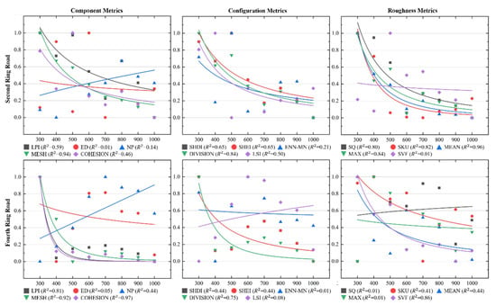
Figure 13.
Power fitting of the normalized CORV of each 3D landscape metric at 30 m grain size.
By comparing the PCC between landscape metrics and LST in Section 3.2 and the feature importance of RFR in Section 3.4, most of the PCC between landscape pattern metrics and LST, accuracy of RFR, characteristic importance of RFR and power function fitting curves of CORV tended to be stable at 700 m. This indicated that the results of most landscape metrics calculated under the 700 m rectangle could better describe the overall 3D landscape pattern of the study area. Although the correlation and regression accuracy between the 3D landscape metrics and LST keep increasing with the increase of rectangle size, the increase of the calculation rectangle inevitably leads to the increase of the calculation time. In the calculation process of our study, especially in the fourth ring road area, the calculation time of all metrics by the 1000 m rectangle is much longer than by 300 m rectangle. Considering all factors comprehensively, the 700 m rectangle is considered as the optimal rectangle size to study the relationship between the urban 3D landscape pattern and LST.
4. Discussion
4.1. Multi-Scale Relationship between 3D Landscape Pattern and LST in the Fourth Ring Road of Beijing
In order to mitigate UHI in Beijing and improve residents’ living conditions, our research used Landsat 8 remote sensing images to retrieve LST, combined with land cover and building height data to calculate the 2D and 3D landscape metrics of Beijing’s fourth road and second ring road at different scales. We used the RFR model to evaluate the effect of the 3D landscape pattern on LST. The 3D metrics can quantify the fluctuation characteristics of the urban surface and the difference between it and the projection plane, which can explain the densely built-up landscape in the urban center effectively.
The UHI effect exists obviously in Beijing, and the effect of 3D landscape metrics on LST is significantly higher than that of 2D metrics [37,65]. About 80% of the surface in the study area is impervious surface with buildings over a large proportion. The height character of buildings may be more strongly related to the spatial distribution of LST and impacted by the shadowing area of tall buildings; the heat accumulation from dense buildings can slow down the air and energy flow in urban canyons [32]. The regression accuracy of land landscape metrics and LST for the volume of high-rise buildings shows that the more information in the larger size of rectangle, the better the response effect of 3D landscape metrics to LST, the better the interpretability. The relationship between 3D landscape patterns and LST is highly related, and the composition and configuration information of the landscape by the 2D landscape showed a significantly worse performance for delineating the relationship between the pattern and LST.
Vegetation and water bodies usually decrease LST effectively [66], and our results showed that the increase of patch diversity and evenness in the rectangle—that is, the increase in vegetation and water patches—could significantly weaken daytime UHI. However, the number of patches in the landscape did not directly affect LST, and the spatial relationship between different patches and the shape and size of individual patches were the main factors influencing LST. During the day time, the urban impervious surface absorbs a lot of energy by solar radiation, which is the main heat source that raises its surface temperature. Vegetation and water can cool down the surface through transpiration and evaporation. Figure 14a,b show the area with the higher LST in the study area. There are more vegetation patches in area (a) than in area (b), but the overall temperature in (a) is still very high. By contrast, in Figure 14c,d, the LST of the area around the fourth ring road, which has a large proportion of vegetation and water, decreased significantly, indicating that increasing the proportion of vegetation and water has a powerful result in weakening UHI. The cooling effect of water and vegetation in the landscape is related to the patch size and shape. Vegetation patches in the second ring road are small and scattered, especially grasslands. Grassland is usually distributed more dispersedly with small patches, and the cooling effect of these small patches is more easily affected by the high temperature of the surrounding large impervious surface patches, resulting in a poor cooling effect. It cannot significantly regulate the LST, and may effectively decrease the LST only when it accumulates into large patches. For a single large patch, the more irregular shape and the increase of the number of other land types on the edge can make the edge effect become more obvious between different patches, accelerate the material and energy exchange capacity between patches and different land types, and decrease the LST within a certain range.
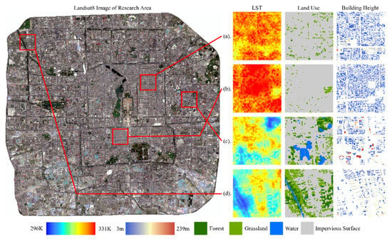
Figure 14.
Comparison of LST, land use and building height in some typical areas of the study area. (a) high LST area with more vegetation; (b) high LST area with less vegetation; (c,d) are low LST area.
The negative correlation between the average height and LST suggested that tall buildings with low density in cities could reduce the summer daytime temperature. The underlying surface absorption of solar energy is the main source of urban surface energy in the summer day, and the shading effect of tall buildings directly reduces the area of direct sunlight [35]. The aerodynamics of low-rise and high-rise buildings are significantly different, with the increase of wind speed; the aerodynamic conductivity of high-rise buildings is higher than that of low-rise buildings, which takes more energy away from its surface and lowers its surface temperature [67]. In addition, the negative correlation between SVF and LST and its high ranking in feature importance explain the influence of building density on LST to a certain extent. For cities, generally, the smaller the SVF value is, the denser the buildings are [68]. In addition to the cooling effect of water and vegetation, the energy exchange between the city and the surrounding suburbs is the main method to reduce LST. The urban structure with high dense buildings tends to slow down the air flow speed of urban canyons, weaken the rate of energy transfer, and make more heat accumulate in the inner city, leading to the rise of LST. Widening urban roads is an important way to improve the SVF and weaken the density of buildings. On this basis, vegetation on both sides of roads and isolated zones can further reduce the LST rises caused by solar radiation.
In general, the change of grain size has little effect on the overall landscape characteristics in the study area as only the accuracy of RFR was improved, while the contribution of different metrics to LST did not change significantly. The change of extent not only causes the change of regression accuracy, but also the regulation of the contribution of metrics. Landscape composition metrics and configuration metrics have a better response effect under large rectangles, while the roughness metrics calculated for buildings had a better interpretation effect under the small rectangle. The larger the research rectangles are, the more stable the dominant land type in the rectangle is, and the calculated landscape composition metrics and configuration metrics can more generally describe the landscape pattern. For our study, the target of the 3D landscape pattern was buildings and the larger rectangle weakened the characteristics of a single building and its influence on the local area, resulting in a lower contribution. However, the result became opposite in the second ring road, especially at the 10 m grain size. It showed that under the high resolution, the purity of each cell increased, and the small study area of the second ring road led to more variation of the factors influencing LST, and each factor had a certain impact on the LST. Meanwhile the overall regulation in the second ring road is similar to other scales, such as SHDI and SHEI, with the highest influence, which also indicated that our study could not only describe the global characteristics of the relationship between the 3D landscape pattern and LST, but also proved that there was a special multi-scale relationship between the two.
Based on our study, combined with the experimental results of landscape metrics and roughness metrics, in order to improve daytime urban thermal environment, we suggest that the distance between urban residential community buildings should be appropriately increased to promote air circulation in future planning. Vegetation area expansion and widening urban roads may absorb radiation and improve the air flow between buildings, respectively. Increasing water and green space can improve inhabitability and benefit residents’ physical and mental health [35].
4.2. Advantages and Limitations
The advantages of our study lie in that 3D landscape metrics were used to study the relationship between LST and the landscape pattern in urban areas, and the calculation size of the rectangle was selected by the spatial variance. However, the resolution of LST based on the remote sensing image is lower than the building target in the study area. In future research, the unmanned aerial vehicle (UAV) monitoring method with thermal infrared band can be considered to obtain a more accurate urban thermal model, urban greening model, 3D surface model and 3D urban model, which can more accurately analyze the relationship between urban landscape and LST. The RFR model is used to regression the 3D landscape metrics and LST, and the regression model based on the tree model shows higher accuracy under large sample conditions and can obtain the feature importance of each metric compared with the ordinary linear regression model. Fifteen landscape metrics were applied to quantitatively describe the landscape pattern of the study area, while more landscape metrics may be selected to describe landscape patterns according to different research conditions and research environments in the future. We studied the multi-scale relationship between LST and landscape patterns under spatial scales, which refers to the change of rectangle sizes and grain sizes. In addition, since the scale-effect includes the spatial scale and time scale, we plan to continue our study in different seasons, year traces and diurnal and nocturnal analysis. We believe that it is of great significance to obtain the effects of 3D landscape characteristics on LST in a series of time changes as well.
5. Conclusions
This paper analyzed the multi-scale relationship between the 3D landscape pattern and LST using random forest regression. According to the experimental results, we indicate that the UHI effect is obvious in the fourth ring road region of Beijing, and the phenomenon of UHI in the central second ring road is stronger than in the fourth ring road, showing an overall trend of diffusion from the center to the surrounding areas. The interpretation effect of 3D landscape metrics on LST was more obvious than that of 2D land-scape metrics, and 3D landscape diversity and evenness played more important roles than the other metrics in the change of LST. The multi-scale relationship between LST and the landscape pattern was discovered in the fourth ring road of Beijing, the effect of the extent change on the landscape pattern is greater than that of the grain size change, and the interpretation effect and correlation of landscape metrics on the LST increases with the increase of rectangle size. The feature importance of the landscape composition and configuration metrics to LST generally increases with the increase of the rectangle, while the contribution of roughness metrics to LST decreases with the increase of the rectangle size. Large areas of vegetation and water are conducive to reducing LST, while small and scattered cooling land types make it difficult to regulate LST. In the summer daytime, tall buildings with a certain distance have a positive impact on decreasing LST because of the shadowing effect, and increasing the distance between buildings helps to increase the heat exchange capacity between the city and the surrounding area, thereby reducing LST.
Author Contributions
Conceptualization, Q.W., Z.L. and F.G.; methodology Q.W., Z.L. and C.Y.; writing—original draft preparation, Q.W. and Z.L.; writing—review and editing, Q.W., Z.L. and H.L.; data curation, Z.L. and L.G. All authors have read and agreed to the published version of the manuscript.
Funding
This research was funded by the National Key Research and Development Program of China (No. 2020YFA0714103).
Institutional Review Board Statement
Not applicable.
Informed Consent Statement
Not applicable.
Conflicts of Interest
The authors declare that they do not have any conflict of interest.
References
- Wang, S.; Hu, M.; Wang, Y.; Xia, B. Dynamics of ecosystem services in response to urbanization across temporal and spatial scales in a mega metropolitan area. Sustain. Cities Soc. 2022, 77, 103561. [Google Scholar] [CrossRef]
- Zhao, L.; Lee, X.; Smith, R.B.; Oleson, K. Strong contributions of local background climate to urban heat islands. Nature 2014, 511, 216–219. [Google Scholar] [CrossRef] [PubMed]
- Rongbo, X.; Zhiyun, O.; Weifeng, L.; Zhaoming, Z.; Gregory, T.J.; Xiaoke, W.; Hong, M. A review of the eco-environmental consequences of urban heat islands. Acta Ecol. Sin. 2005, 25, 2055–2060. [Google Scholar]
- Akbari, H.; Konopacki, S. Calculating energy-saving potentials of heat-island reduction strategies. Energy Policy 2005, 33, 721–756. [Google Scholar] [CrossRef]
- Oke, T.R. Boundary Layer Climates. Earth Sci. Rev. 1987, 27, 265. [Google Scholar]
- Wang, H.; Zhang, Y.; Tsou, J.; Li, Y. Surface Urban Heat Island Analysis of Shanghai (China) Based on the Change of Land Use and Land Cover. Sustainability 2017, 9, 1538. [Google Scholar] [CrossRef] [Green Version]
- Ng, E.; Chen, L.; Wang, Y.; Yuan, C. A study on the cooling effects of greening in a high-density city: An experience from Hong Kong. Build. Environ. 2012, 47, 256–271. [Google Scholar] [CrossRef]
- Figuerola, P.I.; Mazzeo, N.S.A. Urnan-nural temperature differences in Buenos Aires. Int. J. Climatol. 1998, 18, 1709–1723. [Google Scholar] [CrossRef]
- Tan, J.; Zheng, Y.; Tang, X.; Guo, C.; Li, L.; Song, G.; Zhen, X.; Yuan, D.; Kalkstein, A.J.; Li, F. The urban heat island and its impact on heat waves and human health in Shanghai. Int. J. Biometeorol. 2010, 54, 75–84. [Google Scholar] [CrossRef] [PubMed]
- Guo, A.; Yang, J.; Xiao, X.; Xia, J.; Jin, C.; Li, X. Influences of urban spatial form on urban heat island effects at the community level in China. Sustain. Cities Soc. 2020, 53, 101972. [Google Scholar] [CrossRef]
- Patz, J.A.; Campbell-Lendrum, D.; Holloway, T.; Foley, J.A. Impact of regional climate change on human health. Nature 2005, 438, 310–317. [Google Scholar] [CrossRef]
- Sun, L.; Chen, J.; Li, Q.; Huang, D. Dramatic uneven urbanization of large cities throughout the world in recent decades. Nat. Commun. 2020, 11, 5366. [Google Scholar] [CrossRef]
- Liu, X.; Zhou, Y.; Yue, W.; Li, X.; Liu, Y.; Lu, D. Spatiotemporal patterns of summer urban heat island in Beijing, China using an improved land surface temperature. J. Clean. Prod. 2020, 257, 120529. [Google Scholar] [CrossRef]
- Zhao, W.; Gong, H.; Zhao, W.; Tang, T. Spatial Distribution of Urban IP Pollution and CCA Analysis between IP and Meteorological Factors: A Case Study in Beijing. Geogr. Geo-Inf. Sci. 2009, 25, 71–74. [Google Scholar]
- He, X.; Wang, J.; Feng, J.; Yan, Z.; Miao, S.; Zhang, Y.; Xia, J. Observational and modeling study of interactions between urban heat island and heatwave in Beijing. J. Clean. Prod. 2020, 247, 119169. [Google Scholar] [CrossRef]
- Cui, Y.; Yan, D.; Hong, T.; Ma, J. Temporal and spatial characteristics of the urban heat island in Beijing and the impact on building design and energy performance. Energy 2017, 130, 286–297. [Google Scholar] [CrossRef] [Green Version]
- Ye, Y.; Qiu, H. Using urban landscape pattern to understand and evaluate infectious disease risk. Urban For. Urban Green. 2021, 62, 127126. [Google Scholar] [CrossRef] [PubMed]
- Tian, Y.; Zhou, W.; Qian, Y.; Zheng, Z.; Yan, J. The effect of urban 2D and 3D morphology on air temperature in residential neighborhoods. Landsc. Ecol. 2019, 34, 1161–1178. [Google Scholar] [CrossRef]
- Forman, R.T.T.; Godron-Wiley, M. Landscape ecology. Landsc. Arch. 1989, 79, 103–104. [Google Scholar] [CrossRef]
- Song, J.; Du, S.; Feng, X.; Guo, L. The relationships between landscape compositions and land surface temperature: Quantifying their resolution sensitivity with spatial regression models. Landsc. Urban Plan. 2014, 123, 145–157. [Google Scholar] [CrossRef]
- Chen, Z.; Xu, B.; Devereux, B. Urban landscape pattern analysis based on 3D landscape models. Appl. Geogr. 2014, 55, 82–91. [Google Scholar] [CrossRef]
- Bourbia, F.; Boucheriba, F. Impact of street design on urban microclimate for semi arid climate (Constantine). Renew. Energy 2010, 35, 343–347. [Google Scholar] [CrossRef]
- Brring, L.; Mattsson, J.O.; Lindqvist, S. Canyon geometry, street temperatures and urban heat island in Malmö, Sweden. J. Climatol. 1985, 5, 433–444. [Google Scholar] [CrossRef]
- Lengsfeld, M.; Kaminsky, J.; Merz, B.; Franke, R.P.; Eliasson, I. Urban nocturnal temperatures, street geometry and land use. Atmos. Environ. 1996, 30, 379–392. [Google Scholar]
- Oke, T.R. Canyon geometry and the nocturnal urban heat island: Compariso of scale model and field observations. J. Climatol. 1981, 1, 237–254. [Google Scholar] [CrossRef]
- Chun, B.; Guldmann, J.M. Spatial statistical analysis and simulation of the urban heat island in high-density central cities. Landsc. Urban Plan. 2014, 125, 76–88. [Google Scholar] [CrossRef]
- Wu, J.; Shen, W.; Sun, W.; Tueller, P.T. Empirical patterns of the effects of changing scale on landscape metrics. Landsc. Ecol. 2002, 17, 761–782. [Google Scholar] [CrossRef]
- Wu, J. Landscape Ecology; Higher Education Press: Beijing, China, 2007; Volume 2. [Google Scholar]
- Yuan, S.; Xia, H.; Yang, L. How changing grain size affects the land surface temperature pattern in rapidly urbanizing area: A case study of the central urban districts of Hangzhou City, China. Environ. Sci. Pollut. Res. Int. 2021, 28, 40060–40074. [Google Scholar] [CrossRef] [PubMed]
- Yuan, F.; Bauer, M.E. Comparison of impervious surface area and normalized difference vegetation index as indicators of surface urban heat island effects in Landsat imagery. Remote Sens. Environ. 2007, 106, 375–386. [Google Scholar] [CrossRef]
- Hoffman, S. Vegetation as a climatic component in the design of an urban street: An empirical model for predicting the cooling effect of urban green areas with trees. Energy Build. 2000, 31, 221–235. [Google Scholar]
- Huang, X.; Wang, Y. Investigating the effects of 3D urban morphology on the surface urban heat island effect in urban functional zones by using high-resolution remote sensing data: A case study of Wuhan, Central China. ISPRS J. Photogramm. Remote Sens. 2019, 152, 119–131. [Google Scholar] [CrossRef]
- Gage, E.A.; Cooper, D.J. Relationships between landscape pattern metrics, vertical structure and surface urban Heat Island formation in a Colorado suburb. Urban Ecosyst. 2017, 20, 1229–1238. [Google Scholar] [CrossRef]
- Lai, S.; Zhao, Y.; Fan, Y.; Ge, J. Characteristics of daytime land surface temperature in wind corridor: A case study of a hot summer and warm winter city. J. Build. Eng. 2021, 44, 103370. [Google Scholar] [CrossRef]
- Guo, F.; Wu, Q.; Schlink, U. 3D building configuration as the driver of diurnal and nocturnal land surface temperatures: Application in Beijing’s old city. Build. Environ. 2021, 206, 108354. [Google Scholar] [CrossRef]
- Breiman, L. Bagging Predictors. Mach. Learn. 1996, 24, 123–140. [Google Scholar] [CrossRef] [Green Version]
- Yu, S.; Chen, Z.; Yu, B.; Wang, L.; Wu, B.; Wu, J.; Zhao, F. Exploring the relationship between 2D/3D landscape pattern and land surface temperature based on explainable eXtreme Gradient Boosting tree: A case study of Shanghai, China. Sci. Total Environ. 2020, 725, 138229. [Google Scholar] [CrossRef]
- Pais, C.; Miranda, A.; Carrasco, J.; Shen, Z.-J.M. Deep fire topology: Understanding the role of landscape spatial patterns in wildfire occurrence using artificial intelligence. Environ. Model. Softw. 2021, 143, 105122. [Google Scholar] [CrossRef]
- Lin, J.; Lu, S.; He, X.; Wang, F. Analyzing the impact of three-dimensional building structure on CO2 emissions based on random forest regression. Energy 2021, 236, 121502. [Google Scholar] [CrossRef]
- Dai, T.; Qu, Z.; Shi, F. Infrastructure stock in the process of urbanization in Beijing. Alex. Eng. J. 2021, 61, 3277–3291. [Google Scholar] [CrossRef]
- Peng, J.; Xie, P.; Liu, Y.; Jing, M. Urban thermal environment dynamics and associated landscape pattern factors: A case study in the Beijing metropolitan region. Remote Sens. Environ. 2016, 173, 145–155. [Google Scholar] [CrossRef]
- Qin, Z.; Karnieli, A.; Berliner, P. A mono-window algorithm for retrieving land surface temperature from Landsat TM data and its application to the Israel-Egypt border region. Int. J. Remote Sens. 2010, 22, 3719–3746. [Google Scholar] [CrossRef]
- Qin, Z.; Dall’Olmo, G.; Karnieli, A.; Berliner, P. Derivation of split window algorithm and its sensitivity analysis for retrieving land surface temperature from NOAA-advanced very high resolution radiometer data. J. Geophys. Res. Atmos. 2001, 106, 22655–22670. [Google Scholar] [CrossRef]
- Hanqiu, X. Retrieval of the reflectance and land surface temperature of the newly—Launched Landsat 8 satellite. Chin. J. Geophys. 2015, 58, 7. [Google Scholar]
- Liu, L.; Zhang, Y. Urban Heat Island Analysis Using the Landsat TM Data and ASTER Data: A Case Study in Hong Kong. Remote Sens. 2011, 3, 1535–1552. [Google Scholar] [CrossRef] [Green Version]
- Han, Y.; Wang, J.-l.; Li, P. Influences of landscape pattern evolution on regional crop water requirements in regions of large-scale agricultural operations. J. Clean. Prod. 2021, 327, 129499. [Google Scholar] [CrossRef]
- Li, K.; Li, C.; Liu, M.; Hu, Y.; Wang, H.; Wu, W. Multiscale analysis of the effects of urban green infrastructure landscape patterns on PM2.5 concentrations in an area of rapid urbanization. J. Clean. Prod. 2021, 325, 129324. [Google Scholar] [CrossRef]
- Wu, Q.; Guo, F.; Li, H.; Kang, J. Measuring landscape pattern in three dimensional space. Landsc. Urban Plan. 2017, 167, 49–59. [Google Scholar] [CrossRef]
- Li, J.; Zhou, K.; Xie, B.; Xiao, J. Impact of landscape pattern change on water-related ecosystem services: Comprehensive analysis based on heterogeneity perspective. Ecol. Indic. 2021, 133, 108372. [Google Scholar] [CrossRef]
- Wu, Q.; Tan, J.; Guo, F.; Li, H.; Chen, S. Multi-Scale Relationship between Land Surface Temperature and Landscape Pattern Based on Wavelet Coherence: The Case of Metropolitan Beijing, China. Remote Sens. 2019, 11, 3021. [Google Scholar] [CrossRef] [Green Version]
- Mukaka, M.M. Statistics Corner: A guide to appropriate use of Correlation coefficient in medical research. Malawi Med. J. 2012, 24, 69–71. [Google Scholar] [PubMed]
- Lian, J.; Garner, G.; Muessig, D.; Lang, V. A simple method to quantify the morphological similarity between signals. Signal Process. 2010, 90, 684–688. [Google Scholar] [CrossRef]
- Mccullagh, P. Generalized linear models. Eur. J. Oper. Res. 1989, 16, 285–292. [Google Scholar] [CrossRef]
- Breiman, L. Random forest. Mach. Learn. 2001, 45, 5–32. [Google Scholar] [CrossRef] [Green Version]
- Zhu, L.; Zhou, X.; Zhang, C. Rapid identification of high-quality marine shale gas reservoirs based on the oversampling method and random forest algorithm. Artif. Intell. Geosci. 2021, 2, 76–81. [Google Scholar] [CrossRef]
- Xie, Y.; Li, X.; Ngai, E.W.T.; Ying, W. Customer churn prediction using improved balanced random forests. Expert Syst. Appl. 2009, 36, 5445–5449. [Google Scholar] [CrossRef]
- Torre-Tojal, L.; Bastarrika, A.; Boyano, A.; Lopez-Guede, J.M.; Graña, M. Above-ground Biomass Estimation from LiDAR data using Random Forest algorithms. J. Comput. Sci. 2021, 101517. [Google Scholar] [CrossRef]
- Asadi, S.; Roshan, S.; Kattan, M.W. Random forest swarm optimization-based for heart diseases diagnosis. J. Biomed. Inf. 2021, 115, 103690. [Google Scholar] [CrossRef]
- Cho, A. High density biomass estimation for wetland vegetation using WorldView-2 imagery and random forest regression algorithm. Int. J. Appl. Earth Obs. Geoinf. 2012, 18, 399–406. [Google Scholar]
- Hutengs, C.; Vohland, M. Downscaling land surface temperatures at regional scales with random forest regression. Remote Sens. Environ. 2016, 178, 127–141. [Google Scholar] [CrossRef]
- Dongke, L.; Shengyan, D.; Guofu, L.; Qinghe, Z.; Qian, T.; Linghua, K. Landscape heterogeneity of mountainous and hilly area in the western Henan Province based on moving window method. Acta Ecol. Sin. 2014, 34, 3414–3424. [Google Scholar]
- Whittaker, R.H. Vegetation of the Siskiyou Mountains Oregon and California. Ecol. Monogr. Ecol. Monogr. 1960, 30, 279–338. [Google Scholar] [CrossRef]
- Kröger, R.; Khomo, L.M.; Levick, S.; Rogers, K.H. Moving window analysis and riparian boundary delineation on the Northern Plains of Kruger National Park, South Africa. Acta Oecol. 2009, 35, 573–580. [Google Scholar] [CrossRef]
- Logan, T.M.; Zaitchik, B.; Guikema, S.; Nisbet, A. Night and day: The influence and relative importance of urban characteristics on remotely sensed land surface temperature. Remote Sens. Environ. 2020, 247, 111861. [Google Scholar] [CrossRef]
- Zhang, N.; Zhang, J.; Chen, W.; Su, J. Block-based variations in the impact of characteristics of urban functional zones on the urban heat island effect: A case study of Beijing. Sustain. Cities Soc. 2022, 76, 103529. [Google Scholar] [CrossRef]
- Jenerette, G.D.; Harlan, S.L.; Brazel, A.; Jones, N.; Larsen, L.; Stefanov, W.L. Regional relationships between surface temperature, vegetation, and human settlement in a rapidly urbanizing ecosystem. Landsc. Ecol. 2007, 22, 353–365. [Google Scholar] [CrossRef]
- Li, J.; Song, C.; Cao, L.; Zhu, F.; Meng, X.; Wu, J. Impacts of landscape structure on surface urban heat islands: A case study of Shanghai, China. Remote Sens. Environ. 2011, 115, 3249–3263. [Google Scholar] [CrossRef]
- Grimmond, S. Urbanization and global environmental change: Local effects of urban warming. Geogr. J. 2007, 173, 83–88. [Google Scholar] [CrossRef]
Publisher’s Note: MDPI stays neutral with regard to jurisdictional claims in published maps and institutional affiliations. |
© 2022 by the authors. Licensee MDPI, Basel, Switzerland. This article is an open access article distributed under the terms and conditions of the Creative Commons Attribution (CC BY) license (https://creativecommons.org/licenses/by/4.0/).