Automatic Mapping and Characterisation of Linear Depositional Bedforms: Theory and Application Using Bathymetry from the North West Shelf of Australia

Abstract

Bedforms are key components of Earth surfaces and yet their evaluation typically relies on manual measurements that are challenging to reproduce. Several methods exist to automate their identification and calculate their metrics, but they often exhibit limitations where applied at large scales. This paper presents an innovative workflow for identifying and measuring individual depositional bedforms. The workflow relies on the identification of local minima and maxima that are grouped by neighbourhood analysis and calibrated using curvature. The method was trialed using a synthetic digital elevation model and two bathymetry surveys from Australia’s northwest marine region, resulting in the identification of nearly 2000 bedforms. The comparison of the metrics calculated for each individual feature with manual measurements show differences of less than 10%, indicating the robustness of the workflow. The cross-comparison of the metrics resulted in the definition of several sub-types of bedforms, including sandwaves and palaeoshorelines, that were then correlated with oceanic conditions, further corroborating the validity of the workflow. Results from this study support the idea that the use of automated methods to characterise bedforms should be further developed and that the integration of automated measurements at large scales will support the development of new classification charts that currently rely solely on manual measurements.

1. Introduction

Linear depositional bedforms (‘bedforms’ hereafter) are a type of sedimentary structure that form from the action of a fluid flowing over unconsolidated sediments [1,2]. Fluid flow direction can be unidirectional or bidirectional, and the sediments that make up the bedform are typically siliciclastic [3] or bioclastic [4]. Bedforms exhibit a large range of morphologies depending on fluid flow properties, seabed topography, sediment grain size and mode of transport and are usually characterised by ridge-like morphologies [5,6,7]. Bedform size can vary from centimetre scale [1] to kilometre scale [3]. Bedforms often exhibit some level of asymmetry in which case the shorter flank is referred to as the lee side and the longer flank as the stoss side. Asymmetry typically indicates a dominant fluid flow direction, with sediments being transported from the stoss to the lee side [2].

Sub-aqueous bedforms have been extensively studied for decades given that they may represent a significant hazard to navigation and offshore engineering [8,9], a potential target for offshore sand mining [10] or constitute marine habitats [11]. Additionally, their study can help to better understand local hydrodynamics [12], seabed sediment mobility [13,14] and, more largely, surface processes [2].

Over the years, several bedform classifications were created in an attempt to better understand these features [5,15,16,17]. While these classifications provide a basis to study bedforms, they show some limitations as they are based on either manual measurements that can fail to fully capture bedform variability through large areas or do not integrate the full range of quantifiable metrics. In that context, authors have used different approaches to automate bedform identification and quantification. For example, ref. [18] developed a method based on curvature, resulting in the identification of crestlines and troughs as clouds of points. Subsequently, refs. [19,20] also developed methods to identify bedforms as clouds of points but using, respectively, the concept of steepest decent and Fourier analysis, wavelength transform and zero crossing. Other authors further investigated zero crossings [21,22] but along user defined profiles. Similarly, ref. [23] analysed longitudinal profiles to identify a change in derivatives signs while [24], also using longitudinal profiles, used the position of local minima and maxima. Other authors have attempted to use spatial classes (e.g., [25,26,27,28,29]), building on concepts such as geomorphons [30], topographic signatures [31] or index [32], that are then converted into individual features. Finally, other authors explored the delineation of crestline areas by skeletonization using triangular irregular network [33] and polygon breaking algorithms [34,35].

The main limitation of the above methods is that they are either (1) based on user-defined topographic profiles that may not fully capture bedform spatial variability; (2) providing metrics for bedform fields as a whole (e.g., as a cloud of points) and, therefore, do not discriminate individual features; (3) requiring significant manual steps; or (4) not supporting the computation of metrics. In that context, the objective of this research was to develop a tool that could perform the following: (1) identify and discriminate individual bedforms; (2) support the computation of a full range of relevant metrics for each individual bedform; and (3) can be used and reproduced by scientists.

Australia’s northwest marine region (sensu [36]) is affected by strong tidal and oceanic currents [37,38,39,40], cyclone activity [41] and internal waves [42,43], resulting in the formation of widespread bedforms [42,44]. Additionally, recent work indicates that large portions of the shelf are covered by relict coastal features of aeolian and marine origins [45]. The combination of both modern and relict features results in a complex seabed morphology exhibiting a large range of bedforms, making it an area of great interest to develop and trial such automation tools.

Here, we present a new automated approach for bedform detection and quantitative analysis. The workflow was initially developed using a satellite-derived bathymetry (SDB) grid produced over the southern part of Australia’s northwest marine region by [46] and, subsequently, trialed with a synthetic digital elevation model (‘DEM’) and two multibeam echosounder (MBES) bathymetry grids acquired in the vicinity of Broome and of Point Cloates (Figure 1). The study presents the results of this trial and then discusses how such workflow can be used to better understand the nature of bedforms in relation to environmental factors and, in turn, how such tools could be used to improve existing bedform classifications.

2. Materials and Methods

2.1. Datasets

Workflows presented here were developed and trialed using a synthetic DEM and two publicly available MBES bathymetry surveys acquired offshore Broome and Point Cloates along Australia’s northwest marine region.

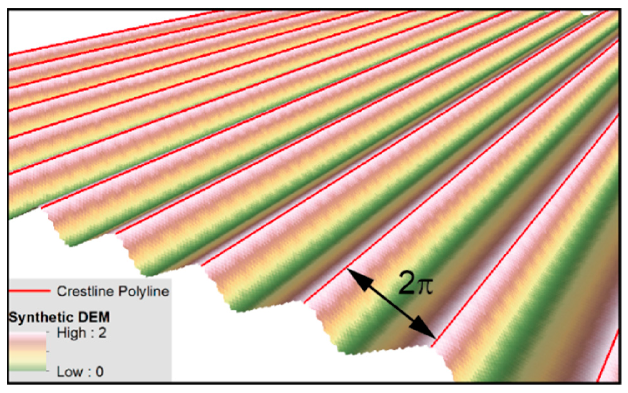
2.1.1. Synthetic DEM

The generation of the synthetic DEM is based on the Equation (1), which was applied along the x axis for each value of Y within a grid of 1000 × 1000 pixels with a pixel size of 0.1 m. The resulting grid was rotated by 45 degrees to simulate an azimuth:

z = sin (x + 0.5 * sin (x)) + 1

(1)

where z corresponds to the elevation value allocated to a pixel, and x corresponds to the position of the pixels along the x axis of the grid.

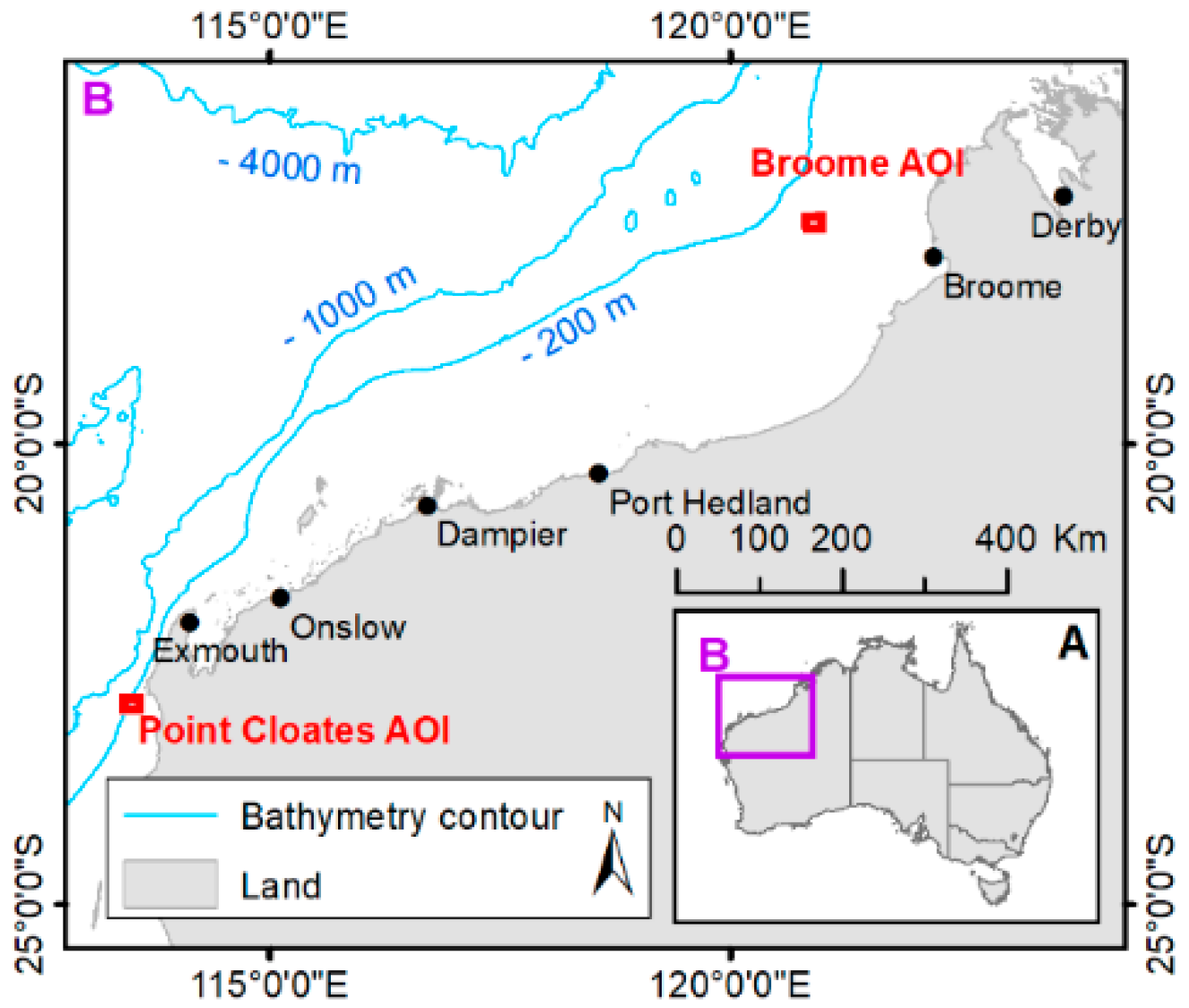
2.1.2. Broome Bathymetry

The bathymetry was acquired in June 2006 by research vessel Southern Surveyor from the Australian Marine National Facility with a Kongsberg Simrad EM 300 multibeam echosounder using a 1° beamwidth and a nominal sonar frequency of 30 kHz [47]. The dataset was accessed through the 5-m bathymetry compilation produced by the National Environmental Science Program [48]. In the area of interest, the bathymetry ranges from 110 to 120 m below sea level (bsl).

2.1.3. Point Cloates Bathymetry

This dataset was acquired by the vessel RV Solander in 2008 as part of a collaboration between Geoscience Australia and the Australian Institute of Marine Science using a Kongsberg Simrad EM3002(D) 300 kHz multibeam sonar [49]. The bathymetry, which ranges from 6 to 192 m bsl, was downloaded as a 3 m grid from the AusSeabed data portal.

2.2. Processing Tools

Processing steps introduced in this paper are all conducted using Python programming language. Scripts were developed based on five key libraries: (1) Arcpy library, available from the ArcMap and ArcGIS Pro software, was used to integrate ArcGIS geo-processing tools in the workflow; (2) Numpy and Pandas libraries were used to manipulate bathymetry grids; (3) Fiona and Shapely libraries, which allow generating and modifying vector files, were used to manipulate shapefiles; (4) the Centreline library, which calculates the centreline of polygons, was used as a starting point to identify crestline polylines; and (5) the Python multiprocessing module was used to split computations between the logical cores of the workstation. Additional libraries were accessed to improve processing steps and are specified in the header of the scripts, which are available as Supplementary Materials.

3. Methods

Automated mapping and characterisation of the bedforms are performed in two steps. First, the input DEM is scanned along the x and y axis to identify stationary points and, in turn, bedform crestlines by using neighbourhood analysis. Second, a high number of perpendicular cross-sections are generated along each crestline polyline to refine its position and identify the base of the bedform on either side of the crestline. These points are then used to calculate bedform metrics. The detailed processing steps are presented in Figure 2 and are described hereafter. While the workflow relies on the use of a licensed Python library, Arcpy, it can presumably be reproduced using any other geographic information system (GIS) software. It should be noted that the workflow requires several user-defined parameters and that, while the following subsections remain generic, these parameters are specified for each case study. Python scripts supporting the workflow are available as supplementary material and consist of the following files: Step0: Generation of tiles; Step1: Identification of bedform polygons; Step2: Generation of bedform crestline polylines; and Step3: Generation of metrics.

Additionally, the term base is preferred over trough throughout the manuscript as the term trough, usually used when describing rhythmic sandwaves, can be misleading when referring to isolated bedforms that are by definition not bordered by depressions.

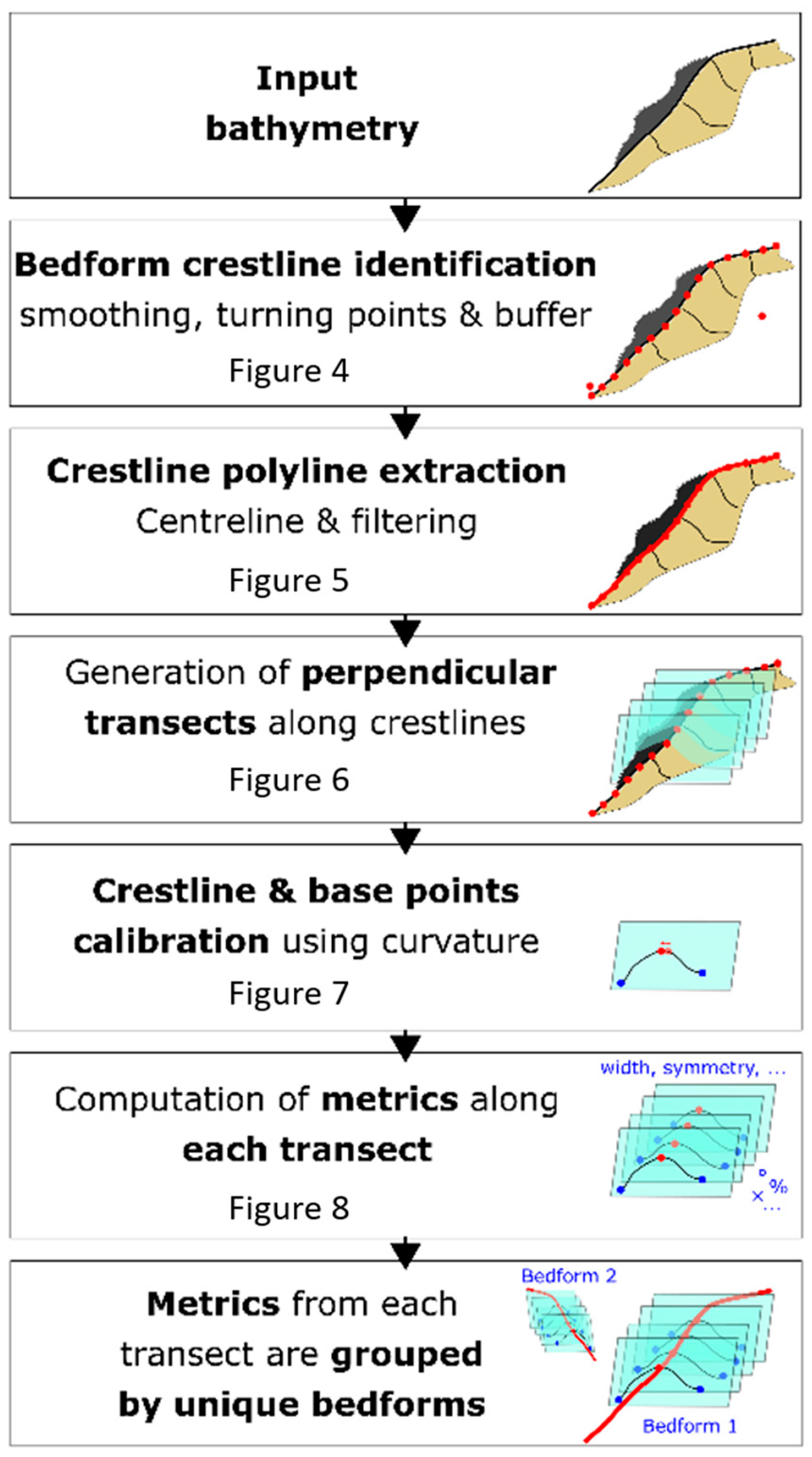
3.1. Extraction of Bedform Crestlines

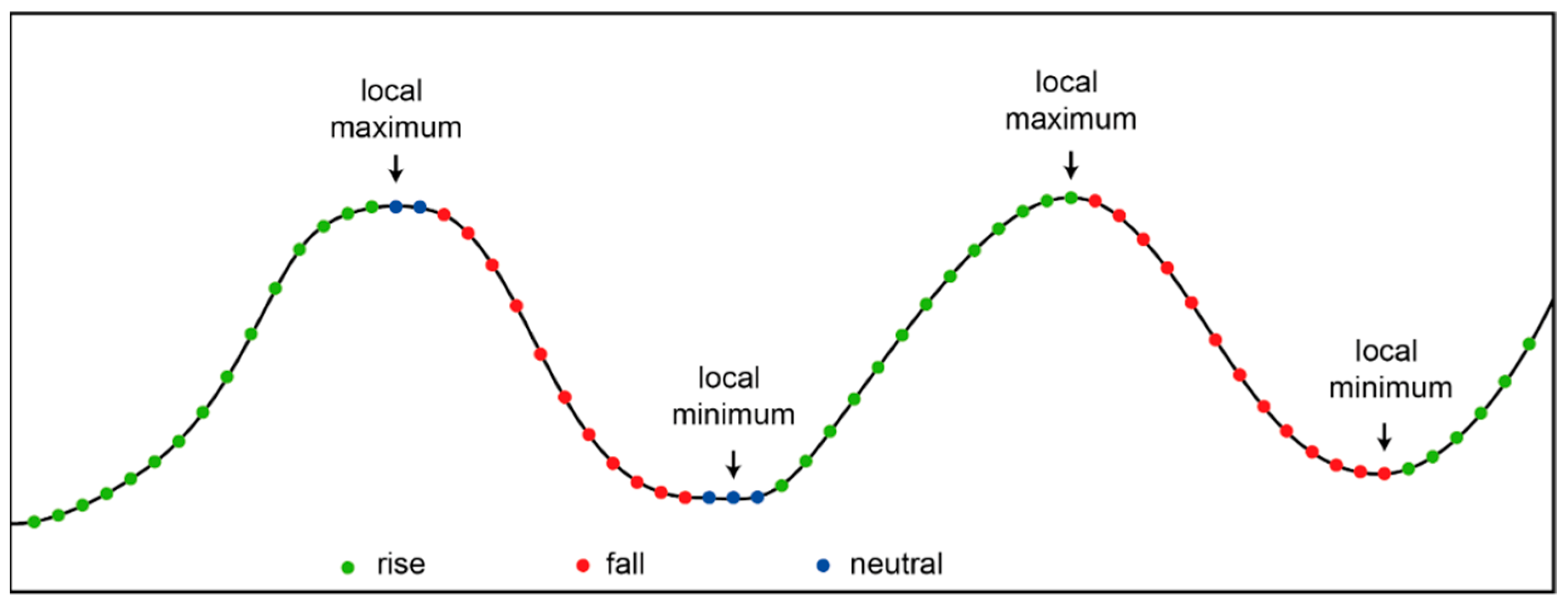
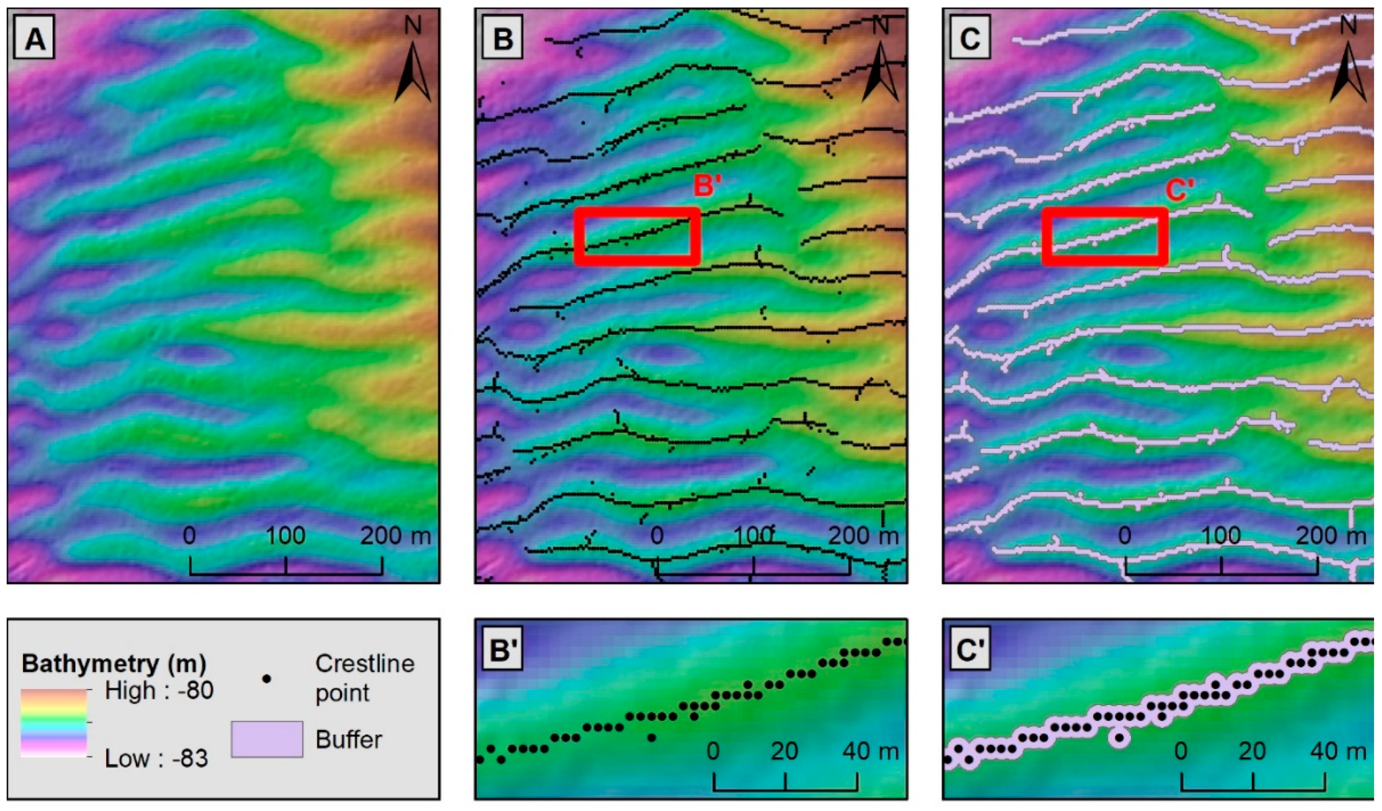
3.1.1. Identification of Bedform Crestline Points

Processing steps presented hereafter can take significant time periods (minutes to hours), depending on the size of the input DEM. To work around that, the DEM is split into smaller overlapping tiles. Tiles are obtained by generating a fishnet for which its cells are buffered by a given distance. The resulting polygons are then used as input to clip the DEM and distribute tiles between the workstation logical cores, hence reducing substantially computation time.

In cross-sections, bedforms can be defined by stationary points where two local minima flank a local maximum [18] (Figure 3). Following this principle, the DEM is screened along the x and y axis to identify such points using a function from [50]. To perform this, each pixel is compared to the preceding pixel and is classified based on the difference between both pixel values: if the difference is positive, the pixel is considered as a rise; if the difference is negative, the pixel is considered as a fall; and if the difference is null, the pixel is neutral. The middle point between a rise and a fall corresponds to a stationary point which is then categorised as either a local maximum or a local minimum depending on whether it is bounded by a rise and a fall or a fall and a rise, respectively (Figure 3).

The number of returned local maxima and local minima varies significantly depending on the noise of the DEM. To ensure that only meaningful points are identified, two levels of filtering are applied: (1) the DEM is smoothed using focal statistics where each pixel is replaced by the average value of surrounding pixels, within a user-defined circular search window; and (2) the height of each bedform is computed using the Pythagoras theorem and stationary point coordinates. Bedforms smaller than a specific user-defined height threshold are discarded. In some instances, multiple bedforms are superimposed. In such cases, modifying filtering parameters can help target specific bedforms based on their respective sizes.

The output is a cloud of points where bedforms are highlighted by clusters of local maxima (Figure 4B) similar to what was achieved by previous methods [18,19,20]. Identified local maxima are independent from each other, meaning that, at this stage, individual points are not associated to a specific bedform. To achieve this, a buffer is generated around each local maximum point, effectively combining them into polygons (Figure 4C). The value of the buffer, in number of cells, can be modified depending on the bedform’s lateral continuity, with wide buffers connecting distant points. To remove outliers that typically result from bathymetry grid artefacts, polygons for which their areas are smaller than the area occupied by a given number of aggregated points are discarded. The relationship between the number of points and the area is approximated using Equation (2) based on the assumption that most bedforms are linear:

A = r² * π + (n − 1) * 2r * p

(2)

where A is the minimum threshold area, r is the radius in metres of the buffer, corresponding to the DEM cell size multiplied by the buffer value, n is the minimum number of aggregated points and p is the pixel size of the DEM.

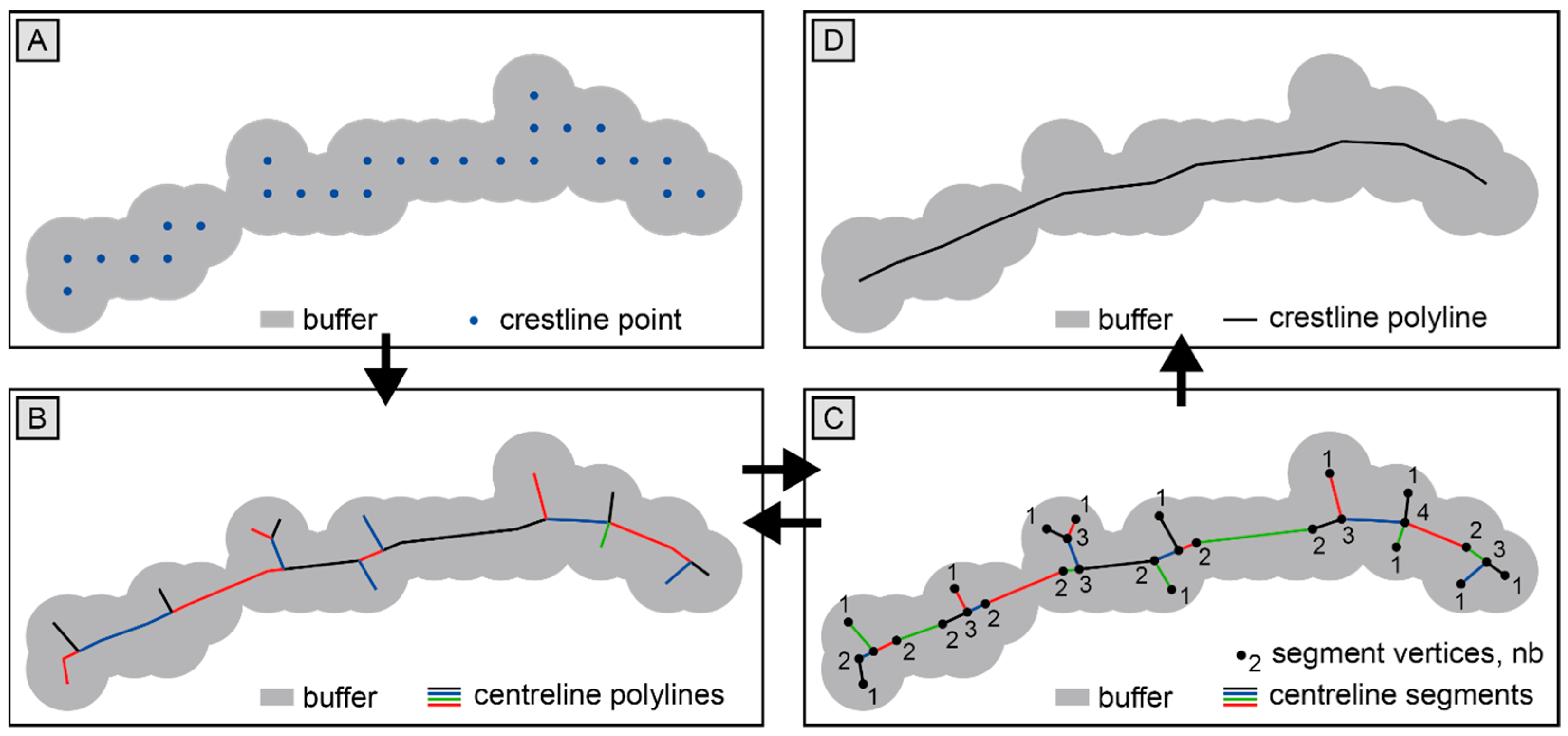
3.1.2. Generation of Crestline Polylines

Individual bedforms are generally characterised by a cluster of points (Figure 5A) meaning that it is not possible to simply link together local maxima points that are part of the same polygon to obtain a crestline polyline. Polygons are, however, centred on the crestline positions. Hence, the centreline of each polygon corresponds to the crestline of the associated bedform. The Python library Centreline creates Voronoi cells from polygon vertices (connecting nodes), densified at specific intervals. The seeds of each Voronoi cell are then connected to generate a centreline.

While this method provides good results with simple polygon geometries, complex geometries often result in the generation of multipart polylines associated with several branches that need to be filtered out (Figure 5B). The identification of branches is based on the analysis of polyline vertices. Polylines are converted to single-part lines (i.e., each individual part has exactly two vertices) meaning that each polyline vertex results in a number of overlapping single-part line vertices. That number corresponds to the number of single-part lines connected to the polyline vertex. Hence, a branch (i.e., a polyline part) is highlighted by the presence of at least three vertices on one end (i.e., the connecting node) and only one vertex on the other (i.e., the end point, Figure 5C). Branches that are shorter than a user-specified threshold are then discarded. Given that branches can themselves have branches, the process is repeated iteratively five times, ensuring that all branches are removed (Figure 5D). While this approach may appear overly complex compared to polygon thinning and smoothing [28] or a branch length reduction [35], it has the advantage of removing all branches while preserving the geometry of the resulting centrelines. Such an approach ensures the best possible fit between the resulting polyline and the actual crestline position.

In some cases, where bedforms are very close to one another, the generation of polygons can create artificial bridges between adjacent features. Such bedforms can be identified by using the same method as for branches, except that bridges will be identified by the presence of at least three overlapping vertices on each endpoints.

3.2. Extraction of Bedform Metrics

The extraction of bedform metrics can be performed using crestline polylines obtained from the previous processing step or any other polyline shapefile. Metrics are calculated in three steps: (1) a very high number of perpendicular transects is generated along each polyline; (2) the positions of the bedform bases and crest are refined along each transect using stationary points, calibrated with the curvature; and (3) metrics are calculated for each unique bedform using the XYZ coordinates of the crest and bases obtained along each transect. Polylines are spread between the logical cores of the workstation to minimise processing time

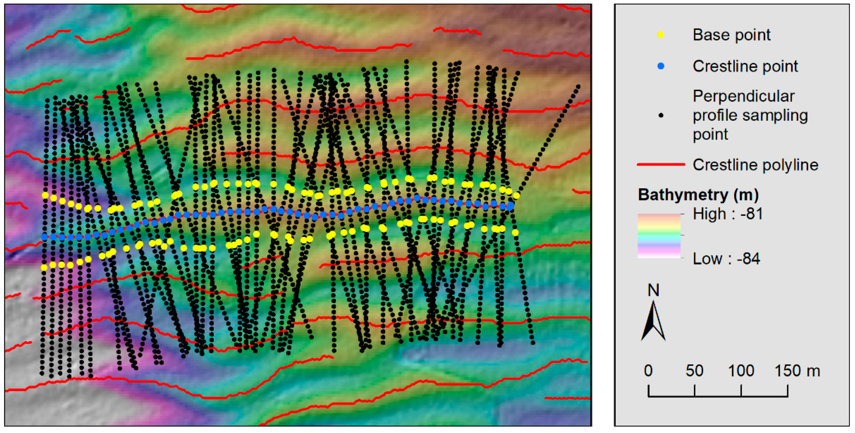
3.2.1. Generation of Perpendicular Transects

It is key to measure metrics perpendicularly to the bedform orientation to ensure that they are not affected by geometrical distortions (e.g., stoss and lee angle measurements made along an oblique cross section will return lower values than reality as well as incorrect width values). In that context, several of the existing methods require user-specified profiles or require rotating the bathymetry [19,20,21,22,23,24]. Here, the script generates perpendicular profiles along crestline polylines to be used as inputs, similar to what was attempted in [28]. To do so, additional vertices are generated along crestline polylines at fixed intervals, typically corresponding to the DEM cell size. The orientation of a line connecting each vertex and the surrounding vertices is calculated using trigonometric rules and then used to generate a perpendicular profile at the vertex’s location. The operation is repeated for all the vertices of each polyline, resulting in a significant number of perpendicular transects (Figure 6). All transects share the same polarity (i.e., they always start and end on the same side of a bedform) to support the computation of orientated metrics such as symmetry index. The length of the profiles can be defined by the user and should be long enough to make sure that the maximum width of all bedforms within the area of interest can be captured.

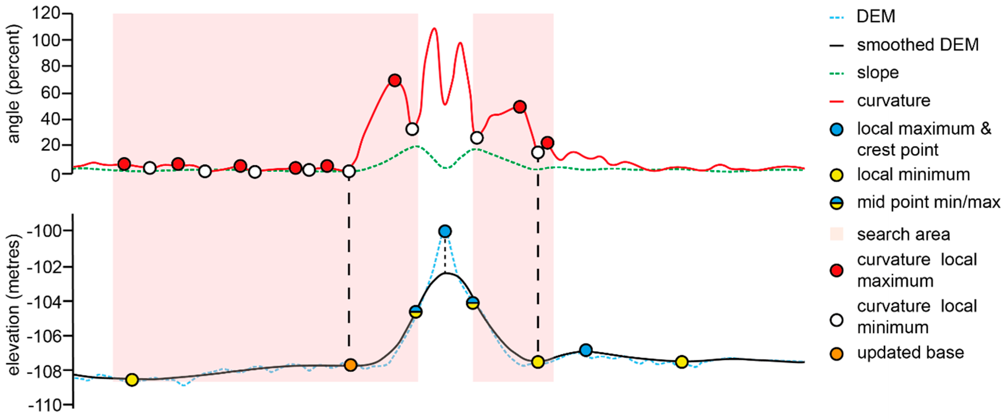
3.2.2. Identification of the Bedform Base and Crestline Points

The Crestline Points computation of metrics is based on identification along each perpendicular transect of three points corresponding to the bedform crestline and associated two bases. While the crestline location was extracted during previous processing steps, it is necessary to update it as it was identified along the x and y axis, which is likely not perpendicular to the crestline orientation and may, therefore, result in inaccurate measurements. The update of crestline position follows the same principle as described in Section 3.1. Topographic profiles are extracted from the re-sampled bathymetry grid along the perpendicular transects to identify local maxima using the function from [50]. For each transect, the local maximum closest to the initial crest location is considered as the updated crestline point. The smoothed DEM, by definition, will return lower height values than the raw data, but the location of the crestline point calculated from the smooth bathymetry may be slightly offset compared to the actual crestline location from raw data, hence potentially returning lower height values as well. To work around this, the highest elevation value between the smoothed DEM and the original DEM is allocated to the crestline point.

On the other hand, the identification of the bedform bases cannot rely solely on the identification of local minima as, in the case of an isolated bedform, the local minima may not correspond to the bases of the bedform [19] (Figure 7). In order to circumvent this possibility, the position of the bedform bases is defined using the second derivative of the bathymetry (i.e., the curvature). At its most basic level, a topographic bedform is defined by two sets of peaks on the curvature corresponding, respectively, to (1) a convex change of topography near the crest of the bedform and (2) a concave change of the topography near the base of the bedform. The identification of curvature peaks corresponding to an increase in slope toward the crestline can, therefore, be used to locate the bases of a bedform. This identification is performed in two steps.

First, a subtransect is selected along each perpendicular transect to carry out curvature analysis to minimise the possibility of identifying false positives. With that intent, elevation local minima are identified along each topographic profile using the method defined in Section 3.1. To remove irrelevant local minima, the depth of each depression associated with a local minimum is calculated using the Pythagoras theorem and the two surrounding local maxima. Local minima associated with depressions of less than a user-specified depth threshold are discarded. For the sake of consistency, this value is the same as the one previously used to discard the smallest peaks. Following this filtering, the two closest local minima on either side of a crestline point are then used to define an interval within which the curvature will be evaluated (Figure 7). As the intent is to identify curvature peaks at the base of the bedform, the interval is further reduced by removing the upper half of the topographic high defined by the crestline point and the two surrounding local minima, resulting in two sub transects on either side of the bedform.

Second, the curvature is analyzed within each of the above defined intervals to identify a curvature global maximum (“CGM”) corresponding to the highest local maximum. The CGM is then evaluated to assess the following:

• Whether it corresponds to a concave change of the bathymetry. In such cases, the elevation of the CGM would be lower than the average elevation of the surrounding values. This criterion is assessed by comparing the elevation of the CGM with the average elevation of the six surrounding values (three on either side).
• Whether elevation values on the crestline side of the curvature local maximum are higher than elevations on the base side in order to ensure CGM is related to the target crest.

If the CGM meets both criteria, it is considered as the reference curvature peak (RCP) on its respective side of the crestline. Otherwise, the process is repeated iteratively with the next highest local curvature maxima until a curvature local maximum meets both criteria. In the unlikely case that none of the curvature local maxima meet the above-mentioned criteria, the CGM is used as RCP. The curvature local minimum located on the base side of the RCP, which correspond to the point where the slope becomes constant, is defined as the bedform base. As for the crestline point height, the elevation of the bedform base will likely be affected by a smoothing effect resulting in overestimated elevation values. The smallest elevation value between the original or smoothed DEM is, therefore, allocated to the point. Following this processing step, each transect along a given polyline is associated with the XYZ coordinates of a crestline and of two bases (Figure 6).

3.2.3. Computation of the Metrics

Bedform metrics are computed using the XYZ coordinates of the crestline and base points calculated along each perpendicular transect. Two types of metrics can be discriminated: (1) transect metrics and (2) planar metrics. Transect metrics are calculated along each transect and the median value from all transects is allocated to the bedform (e.g., width, height and symmetry). For such metrics, it is key to filter out outliers as they typically result from bathymetry data artefacts such as data gaps, acquisition overprint, etc. In that context, the median value was preferred over the average value given that the median is less susceptible to outliers than the average. Planar metrics are calculated using crestline spatial coordinates (e.g., length, orientation and sinuosity index).

The current workflow includes the following metrics: length, sinuosity index, orientation, width, height, symmetry index and base elevations, as well as width/length/height ratios. The definition of each metrics is presented below and, in the case of transect metrics, illustrated in Figure 8:

• Length: Cumulative distance between crestline points;
• Sinuosity index: Total length divided by the distance between the first and last crestline point of a bedform, sensu [51];
• Orientation: Azimuth of the line connecting the first and last crestline points;
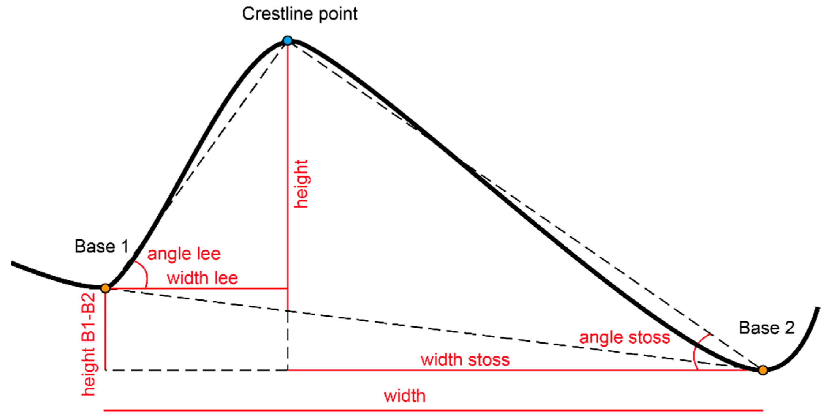
• Width: Distance between both bases, along a horizontal plan;
• Width Lee/Stoss: Distance between the respective base and the associated crestline point, along a horizontal plan;
• Angle Lee/Stoss: Angle between a line joining a base and the associated crestline point and the horizontal axis, on either side on the bedform;
• Height: Difference in elevation between a crestline point and a point marking the intersection of a vertical line going through the peak and the line connecting both base points, calculated using a regressive function connecting both bases;
• Symmetry index: Ratio between the lee and stoss side. The direction of the asymmetry is indicated by the field symmetry direction, which specifies the direction of the lee. A value of 1 indicates a symmetrical bedform while a value > 1 highlights an asymmetrical bedform;
• Length to width ratio: Length divided by width;
• Width to height ratio: Width divided by height;
• Length to height ratio Length divided by height;
• Base elevations: Elevation of each base.

4. Results

The validity of the proposed workflow and of the associated scripts is assessed using a synthetic DEM and two bathymetry grids from Australia’s northwest marine region offshore Broome and Ningaloo Reef (Figure 1).

4.1. Case Study 1: Synthetic DEM

The synthetic DEM, generated using a sinusoidal function, was used as part of the development of the workflow to trial the validity of the concept. The analysis focused on the width, height, symmetry and orientation of the bedforms as these metrics can be theoretically determined for the synthetic DEM. Additionally, these values are directly related to the XYZ coordinates of bedform crestlines and bases from which all metrics are calculated.

The width of the synthetic DEM bedforms corresponds to the period of the sin function, which is of 2π, and can be approximated to 6.28 m. Similarly, the bedforms height correspond to twice the amplitude of the sin function and is equal to 2 m. The determination of the theoretical symmetry index is less straightforward as it relies on the resolution of the Equation (1) for z = 0 and z = 2 to identify the crest and bases of the synthetic bedforms. Given that sin (x) is a transcendental function, it is not possible to solve Equation (1) algebraically and it requires a numerical approximation. This was performed by calculating the position of the maximum and minimum values returned by the equation within an interval of 2π using a sampling rate of 0.01. The positions of the crest and bases were subsequently used to calculate the width of both the lee and stoss sides and the symmetry index. Performing this returned a theoretical symmetry index of 1.8. Finally, bedforms have an orientation of 45 degrees, corresponding to the angle by which the synthetic DEM was rotated. In total, the synthetic DEM contains 12 bedforms.

Given that the synthetic DEM is exempt of noise, the identification of crestline locations was performed without re-smoothing the data and with a minimum bedform height threshold of 0.1 m. Additionally, nominal coefficients of 2 and 10 were used for neighbourhood analysis and for the minimum bedform length threshold, respectively. The proposed method appears to fully capture the crestline position of all 12 bedforms and no significant offsets can be observed between bedform crestline locations and generated crestline polylines (Figure 9).

Bedform metrics were then calculated using the generated crestline polylines as input. The analysis returned median values of 1.99 m, 6.26 m, 1.78 m and 44.99 degrees for the bedform height, width, symmetry index and orientation, respectively (

Table 1. Comparison of the theoretical and computed metrics.

	Theory	Automated
n	12	12
height	2 m	1.99 m
width	6.28 m	6.26 m
symmetry	1.80	1.78
orientation	45°	44.99°

). There is a good match between theoretical and computed values, which supports the validity of the concept.

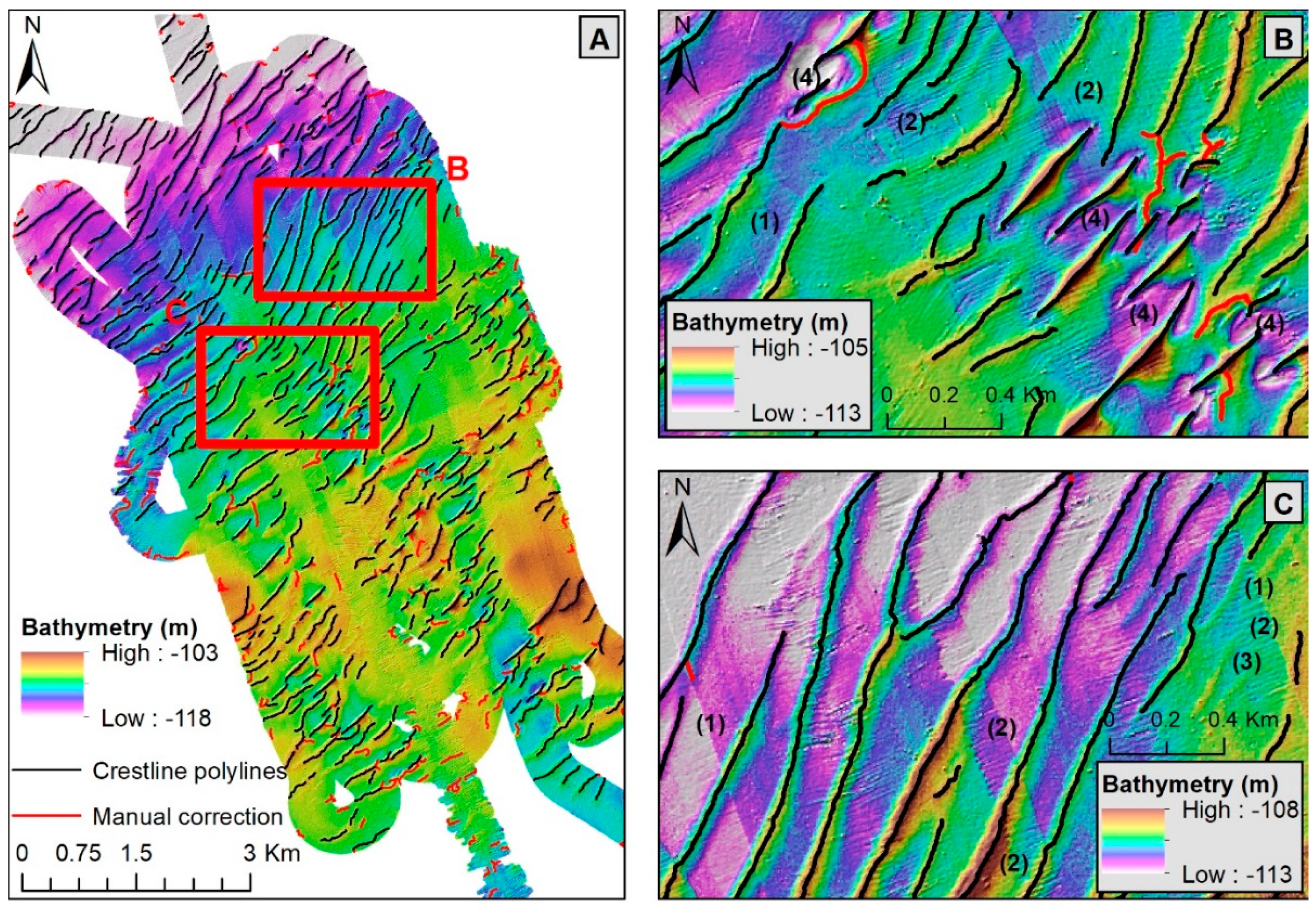
4.2. Case Study 2: Broome

4.2.1. Bedform Identification

The bathymetry grid from the Broome area exhibits multiple processing artefacts that are visible in the form of linear strips, which likely correspond to acquisition corridors, often characterised by vertical offsets in excess of 1 m (Figure 10). Additionally, the bathymetry grid appears quite noisy and it is locally possible to distinguish swath bands (linear artefacts perpendicular to the main acquisition corridors, Figure 10). It was previously reported that bedforms in this area have a height varying between 3.1 and 6.7 m and a width comprised between 90 and 133 m (i.e., between 18 and 27 pixels) [47]. In that context, bathymetric artefacts could potentially affect the output from the automated mapping workflow. To work around that, strong filtering parameters were used, including a smoothing of four (i.e., each smoothed pixel is calculated as the average of all pixels within a radius of four pixels) and a minimum bedform height of 0.5 m. Crestline points were then aggregated with neighbouring points within a radius of 2.1 pixels to obtain crestline polygons and polylines. Finally, all polygons and polylines corresponding to a length of less than 20 pixels were discarded.

Based on a visual inspection, the resulting polylines appear to accurately capture bedforms (Figure 10). Locally, the tool identified relative topographic highs that do not correspond to depositional bedforms and that may be related to local seabed scouring or bathymetry artefacts. Such features, which are considered as false positives, are generally grouped within small areas and were removed manually. Overall, false positives represent, based on the length of the polylines, 16.2% of the identified crestline polylines. Finally, few bedforms appear to have not been captured by the tool. They correspond to features that have a height below the minimum height threshold. Following the manual cleaning of the crestline polylines, the automated workflow resulted in the identification of 381 bedforms.

4.2.2. Calculation of Metrics and Classification

Crestline polylines previously generated were used as input to calculate bedform metrics. The computation of metrics is built on the same filtering parameters previously used to identify crestline polylines. Perpendicular transects, which are generated to compute metrics, were spaced by 10 m (twice the pixel size) and had a length of 800 m.

Metric accuracy was assessed by comparing width, height and symmetry index values obtained from the automated workflow with manual measurements. To perform this, three bathymetry profiles were extracted perpendicular to the main bedform’s orientation. The width, height and the symmetry index of each bedform were manually measured along each profile and compared with the values from the closest automated perpendicular transect, meaning that manual measurements are not compared with the bedform median value but with the closest spot measurement. Such an approach is critical because, while the median bedform value is representative of the bedform, it may locally differ from spot measurements which would result in an incorrect assessment. A total of 21 bedforms were identified from both automated and manual identifications. On average, the absolute differences in height and width between automated and manual measurements are of 8.79% and 9.09%, respectively, while the difference in symmetry index is of 18.42% (

Table 2. Comparison of the manual and automated metrics over Broome area bathymetry.

n	Delta Height	Delta Width	Delta Sym.	Delta Dir.
22	8.79%	9.09%	18.42%	9.05°

).

The automated computation of the metrics resulted in the discrimination of two types of bedforms (Figure 11). The distinction between both types is especially clear from the comparison of width and height (Figure 12A). Metrics are presented in

Table 3. Automated metrics (median value) from Broome area bathymetry. Manual measurements are from [47] and were modified to make both methods comparable.

Metrics		n	Width (m)	Height (m)	W/H Ratio	Length (m)	L/W Ratio	Orientation (deg.)
Type 1	Auto	283	160	1.90	79.19	362.30	2.29	38.19°
	Manual	20	133	3.1	43.8	1306	10.2	Na
Type 2	Auto	98	90	4.41	21.2	275.50	3.22	44.41°
	Manual	20	90	6.7	13.5	402	4.7	Na
Metrics		Angle lee (deg.)	Angle stoss (deg.)	W lee (m)	W stoss (m)	Sym. ind.	Sym. dir. (deg.)	Sinuosity ind.
Type 1	Auto	1.72	1.31	65	85	1.26	301	1.12
	Manual	5.0	3.0	53.2	80.2	1.66	Na	Na
Type 2	Auto	5.84	4.94	40	50	1.17	139	1.1
	Manual	12.3	8.8	42.2	47.2	1.42	Na	Na

, and the most significant ones are described in the text hereafter.

Type 1 bedforms include 283 bedforms with a width to height ratio in excess of 46. These bedforms exhibit a median width of 160 m, height of 1.90 m and length of 362.30 m. Overall values of height, width and length appear quite scattered; however, all bedforms exhibit similar lee and stoss angles varying between 0.66 and 4 and 0.3 and 2.6 degrees, respectively. Finally, Type 1 bedforms are slightly asymmetrical with the stoss side 26% wider than the lee side.

Type 2 bedforms include 98 bedforms with a width to height ratio of less than 46. These bedforms are generally narrower (width), shorter (length) and taller (height) than Type 1 bedforms. They exhibit a median width of 90 m, height of 4.41 m and length of 275.5 m. While the width of Type 2 bedforms is relatively constant, the height varies significantly between 1 and 7.5 m, which results in scattered lee and stoss angle values varying between 2.2 and 9.3 and 2.1 and 8 degrees, respectively. Type 2 bedforms are also slightly asymmetrical but less than Type 1 bedforms with the stoss side on average 17% wider than the lee side. Finally, the height of Type 2 bedforms appears to be reducing with increasing water depths.

Both types of bedforms identified using the automated workflow matches the bedform classification performed by [47] based on 40 manual measurements. While some discrepancies exist between the reported values of each bedform types, it is possible to observe the same trends with, for example, Type 2 bedforms two times higher than Type I bedforms (Table 3).

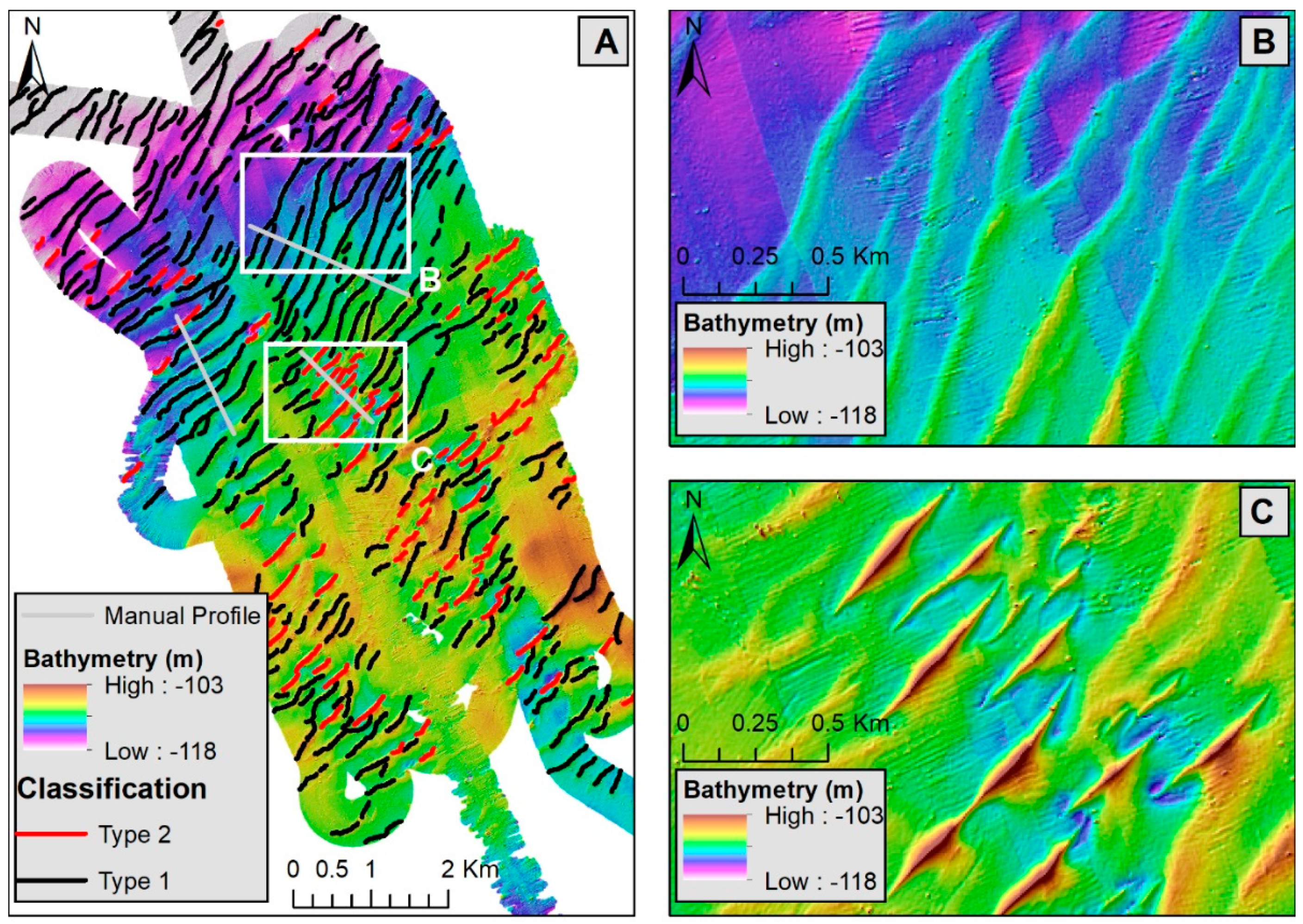
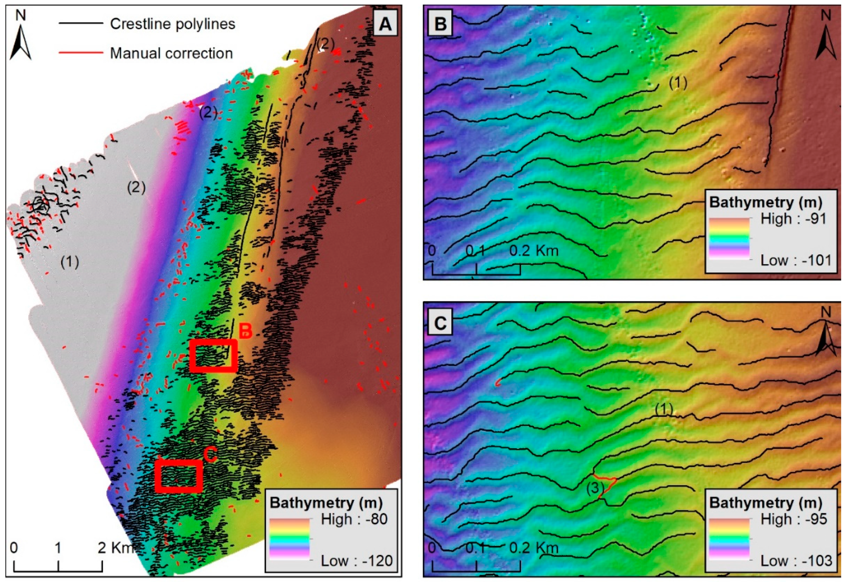
4.3. Case Study 2: Point Cloates

4.3.1. Bedform Identification

The bathymetry from Point Cloates area is of good quality and only exhibits few artefacts at the boundary between acquisition transects. Such boundaries are sometimes illustrated by data gaps and are usually not associated with any vertical offsets (Figure 13). A preliminary manual inspection of the data suggests that most bedforms have a height of less than 1 m and a width varying between 75 and 100 m (i.e., 25 to 35 pixels). In that context, filtering parameters were used to extract crestline points including a smoothing of four pixels and a minimum bedform height of 0.1 m. Subsequently, crestline points were aggregated within a radius of 1.4 pixels. Finally, all polygons and polylines corresponding to a length of less than 20 pixels were discarded.

A visual review of the resulting crestline polylines suggests that the automated workflow accurately captured most of the bedforms (Figure 14). Locally, false positives can be observed either in relation to bathymetry artefacts or where the tool attempted to connect nearby crestline polylines. Such features were removed manually. Overall, false positives amount for 7.5% of identified features, based on polylines length, and are concentrated over specific areas, either at the boundaries of the bedforms fields or of data gaps (e.g., western end of the area of interest). Following the manual cleaning of the crestline polylines, the automated workflow resulted in the identification of 1579 bedforms.

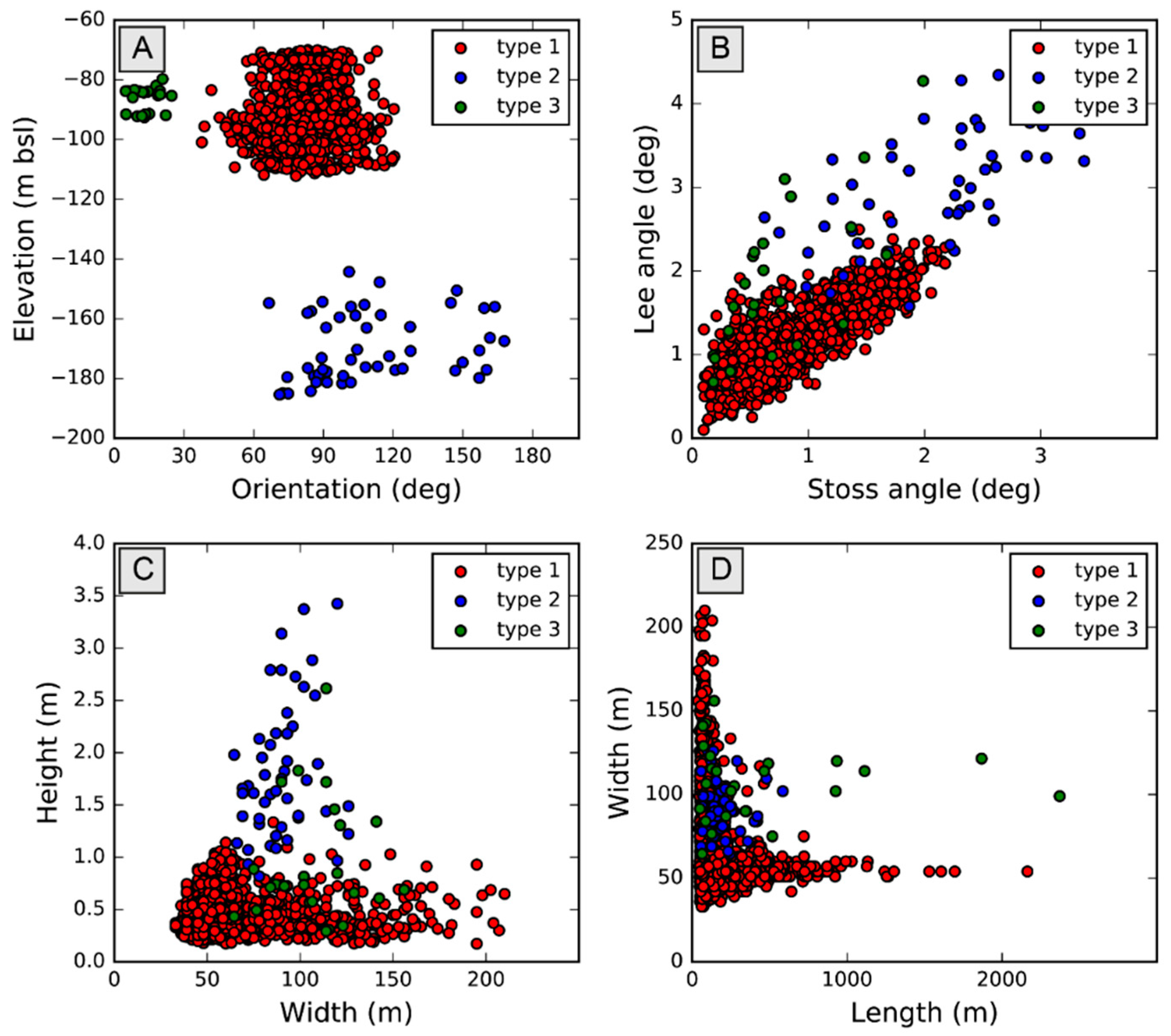
4.3.2. Calculation of Metrics and Classification

Crestline polylines were used as input to calculate bedform metrics, and their computation relied on the same filtering parameters as for bedform identification. Perpendicular transects used to compute metrics were spaced by 10 m and had a length of 300 m.

In order to evaluate the accuracy of the metrics, bedform width, height, and symmetry index were manually measured along a bathymetry profile perpendicular to the main bedform orientation and compared with metrics obtained from the automated workflow (Figure 14). To ensure the validity of the comparison, each manual measurement is compared with the closest automated spot measurement made along each crestline polyline. In total, 38 bedforms were identified from both automated and manual identification. On average, the absolute difference in height and width between both methods is of 5.95% and 4.37%, respectively, while the difference in symmetry index is of 10.88% (

Table 4. Comparison of the manual and automated metrics over Point Cloates area.

n	Delta Height	Delta Width	Delta Sym.	Delta Dir.
38	5.95%	4.39%	10.88%	10.86°

).

The cross-comparison of metrics allows identifying three distinct bedform types (Figure 14). The boundaries between each type are based on the comparison of the bedforms orientation and elevation (Figure 15A). Metrics are presented in

Table 5. Automated metrics (median value) from Point Cloates bedforms.

Metrics	n	Width (m)	Height (m)	W/H Ratio	Length (m)	L/W Ratio	Orientation (North)
Type 1	1506	56.99	0.45	129.82	125.55	2.09	82.82°
Type 2	49	89.99	1.65	50.16	155.16	1.81	101.85°
Type 3	24	110.24	0.73	132.47	187.30	2.04	13.87°
Metrics	Angle lee (deg.)	Angle stoss (deg.)	L. lee (m)	L. stoss (m)	Sym. Ind.	Sym. Dir.	Sinuosity ind.
Type 1	1.09	0.82	24	30	1.25	173.6	1.05
Type 2	2.99	2.26	33	51	1.49	177.48	1.11
Type 3	1.61	0.57	24	79	3.33	103.87	1.04

, and the most significant ones are described below.

Type 1 bedforms include 1506 features that are well developed in depth ranging from 70 to 115 m bsl. All Type 1 bedforms appear to be part of the same field and have an orientation, with the exception of a few outliers, varying between N60 and N120. These bedforms are characterised by a median height of 0.45 m with most of the bedform exhibiting height values below 1 m. Width values appear quite scattered between 25 and 300 m for an average of 57 m. Additionally, Type 1 bedforms have a median length of 125.55 m. Interestingly, it appears that only bedforms of a specific width can reach the highest length values. Finally, these bedforms are moderately asymmetrical with the stoss side 25% wider than the lee side.

Type 2 bedforms include 49 bedforms that are developed at depth varying between 140 m to 190 m bsl. Type 2 bedforms appear to be only partially captured by the tool due to numerous data gaps, which also likely affected the computation of their metrics. Nevertheless, Type 2 bedforms exhibit distinctive metrics with a median height of 1.65 m for a median width of 90 m. As a result, the width to height ratio is much smaller than for Type 1 bedforms. These bedforms have a median length of 155.16 m and a moderate symmetry index of 1.49. Finally, slightly higher sinuosity index values illustrate the bedform’s crescent shape. The bathymetry over the area occupied by Type 2 bedforms presents several data gaps, which are likely affecting the reliability of the metrics.

Type 3 bedforms differ significantly from Type 1 and Type 2 because they are developed almost perpendicular to them with a median orientation of 13.87 degrees. Two distinct sets of bedforms can be identified at 82 and 90 m bsl (Figure 15). In both cases, bedforms are highly asymmetrical with the stoss side generally 333% wider than the lee side. Additionally Type 3 bedforms have a median length of 187.30 m. This number appears underestimated as bedforms within both sets appear to be aligned and might, constitute different segments of the same object that would, therefore, be much longer. Finally, these bedforms exhibit height and width values varying between 0.25 m and 2.5 m and 50 m and 250 m, respectively.

5. Discussions

5.1. Bedform Identification

The delineation of bedform crestlines through the identification of stationary points and subsequent neighbourhood analysis appears to be a precise and reliable approach for mapping submerged linear bedforms. All bedforms with heights and lengths above the specified threshold were identified using Point Cloates and Broome datasets, which included bedforms of variable properties, sometimes heavily affected by data artefacts.

The key advantage of the proposed workflow is that it allows identifying and extracting individual features instead of processing bedform fields as a single object. This approach works particularly well for linear bedforms but may show limitations when attempting to isolate non-linear objects. The workflow assumes that each polygon generated through the neighbourhood analysis is a unique feature that can be reduced to a polyline (i.e., the centreline). If a bedform exhibits several branches, this approach implies that it will either (1) become oversimplified with only the main one properly delineated or, (2) each branch will be regarded as a unique feature because polylines can only have one start point and one end point.

The implementation of a double filtering approach using both a smoothing of the DEM and a minimum bedform height threshold helped to efficiently identify bedforms despite significant data artefacts. This approach should also allow targeting superimposed bedforms using different filtering parameters. This was, however, not tested in this study due to the absence of well-expressed superimposed bedforms. Smoothing values should be set with caution given that a high level of smoothing will modify the geometry of bedforms and may result in inaccurate measurements. Similarly, the minimum bedform height threshold shows some limitation as it does not allow differentiating data artefacts from small bedforms resulting in some of the smaller bedforms being ignored. In that regard, alternative filtering techniques building, for example, on 2D Fourier analysis [20] could potentially enhance results by better isolating data artefacts and enabling a more accurate distinction of superimposed bedforms.

5.2. Generation of Metrics

The computation of metrics using crestline polylines provides the opportunity to obtain accurate metrics for numerous individual features. In that regard, the integration of curvature analysis to supplement the identification of stationary points and, in turn, of bedform bases is key to study each bedform independently from each other. The generation of a high number of perpendicular profiles along each bedform ensures that the resulting metrics are representatives of the entire bedform.

The comparison of the bedform width and height values obtained by using the automated workflow and by manual measurements shows an overall good agreement with average differences negligeable for synthetic DEM (i.e., below 0.2%) and below 10% for both Broome and Point Cloates areas. These differences can be related to the variation of bedforms orientations: All individual bedforms exhibit slightly different orientations. As such, manual profiles extracted through an entire field cannot be perfectly perpendicular to each individual bedform, whereas automated transects are. In that regard, manual profile orientations differ on average by 9 degrees compared to automated transects, which could be sufficient to generate such discrepancies. Symmetry values appear to show more variability, with variation between the manual and automated measurements of 10.88% and 18.42% for Point Cloates and Broome areas, respectively, while remaining negligeable (below 0.025%) for the synthetic bathymetry. Such discrepancies could be the result of the ratio between the pixel size and width of the bedforms. For both test sites, the pixel size was equivalent to approximately 5 to 10% of the bedform’s width. As a result, when calculating the ratio between the lee and stoss sides, an offset of one pixel can significantly affect output values. For example, if the lee and stoss sides are of 21 and 30 m, or of 24 and 27 m, the symmetry will vary by 26% from 1.42 to 1.12. Lastly, Point Cloates metrics appear more accurate than Broome area metrics, which can be explained by the numerous artefacts observed over Broome area bathymetry.

Over the Broome site, the comparison of automated metrics obtained in this study with manual measurements previously published [47] show higher variability with, for example, manual height values nearly doubling automated measurements. However, only a single manual measurement was reported by the authors on each of the 40 bedforms [47] while the automated metrics built on tens of thousands measurements. Additionally, it is likely that they measured bedforms at their apex, effectively reporting maximum values, whereas the automated workflow computed median values along entire bedforms, including data points from the narrower and smaller extremities, hence explaining the differences. In any cases, both sets of metrics highlight similar trends.

Finally, the statistical method retained to allocate a specific value to a bedform from the perpendicular transect measurements can affect results. In some instances, spot measurements can return incorrect values, mainly due to data artefacts or inappropriate parameters. In order to limit the effect of such artefacts, each bedform was allocated the median value from the measurements made along perpendicular transects, as the median is less susceptible to outliers than the average. However, the median also has statistical bias and may not properly capture bedform with complex geometries (e.g., [52]). The computation of the metrics could, therefore, be improved by adding more advanced outlier removal techniques such as interquartile ranges or by including segmented analysis (e.g., width of the bedform first third versus width of the last third).

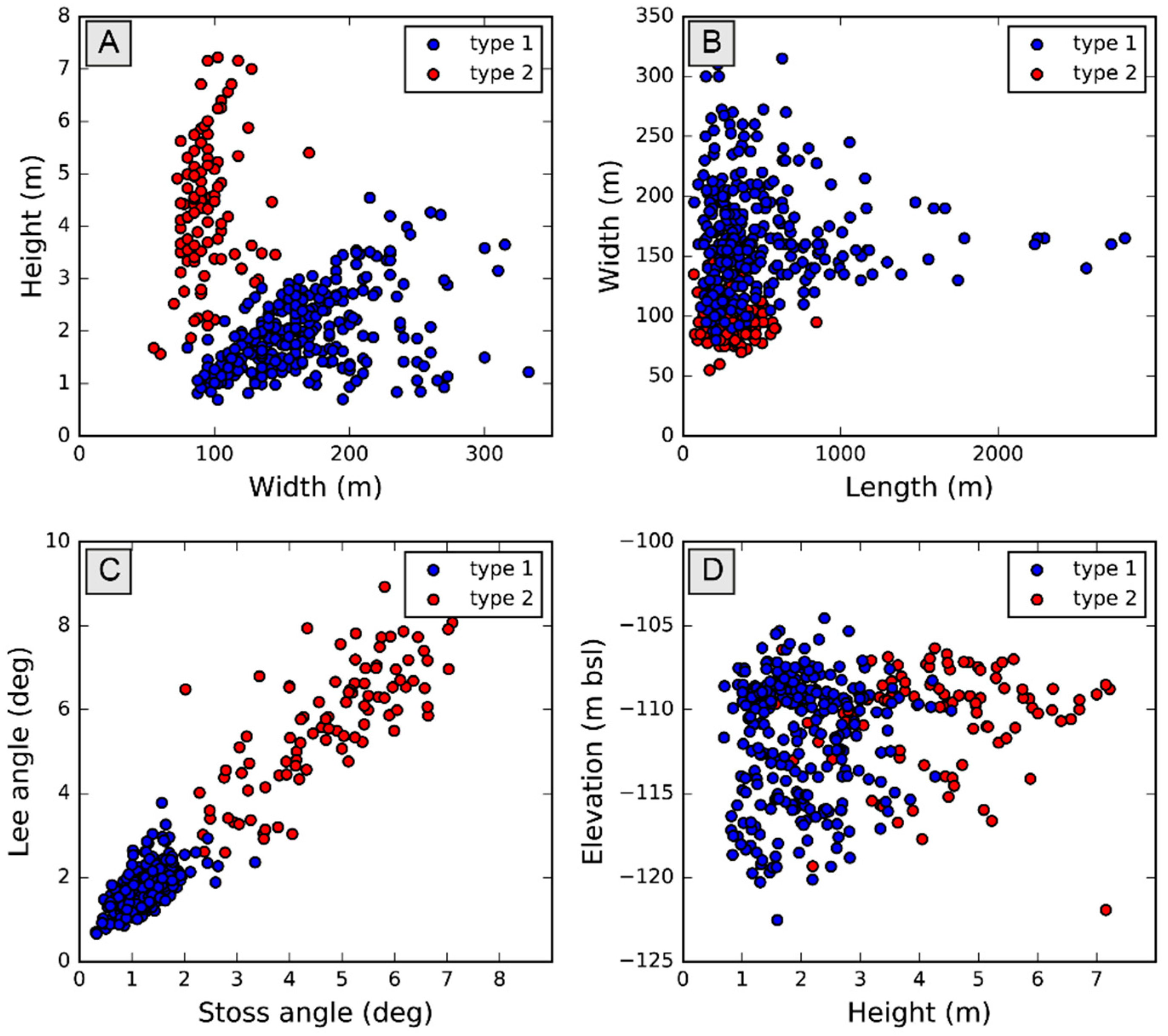
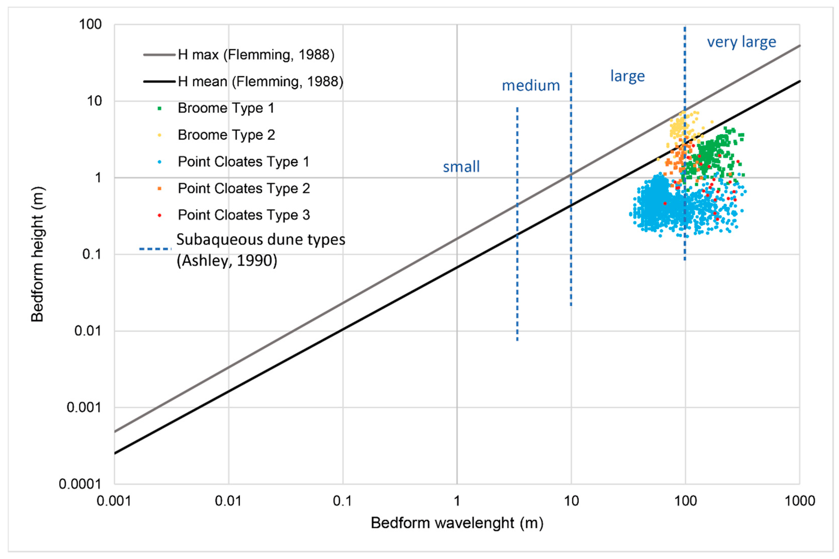
5.3. Comparison of Bedform Properties

The computation of metrics allows subdividing and classifying bedforms. Resulting subsets can then be related to specific geological and oceanographic processes.

In the Broome dataset, bedforms appear perpendicular to the main published tidal current direction (constituent M2) [53]. In addition, bedforms exhibit low symmetry index values and are facing either the northwest or southeast directions, indicating that they were formed by bidirectional currents. The above suggests that bedforms were formed by tidal processes, in line with previous interpretations [47]. The predominance of northwest facing features, highlighting a seaward migration, would indicate that ebb tidal currents are stronger than flood tidal currents. While formed by similar processes, bedforms Type 1 and 2 have different morphologies. Type 1 bedforms (Figure 11B) have similar morphologies and metrics to trochoidal dunes reported in the Leveque Shelf (bedforms ‘Type III’ [54,55]), whereas Type 2 bedforms (Figure 11C) appear closer to the sinusoidal and bifurcated ridges equally reported along the Leveque Shelf (i.e., bedform ‘Type I’ from [54]). Additionally, bedforms Type 2 form prominent fields, while Type 1 bedforms only form localised clusters. The differences between bedform types could result from differences in seabed sediment characteristics and/or availability. Alternatively, given that it is not known whether these bedforms are still active, such differences might indicate that both bedform types are diachronous and were formed under different flow regimes.

Bedforms Type 1 and Type 2 identified within the Point Cloates dataset are also perpendicular to the main direction of the tidal component M2 reported by [53], suggesting that their formation could also be related to tidal processes. Moreover, Type 1 bedforms (Figure 14B) often face opposite directions, indicating that they result from bidirectional currents, hence confirming a tidal origin. On the other hand, Type 2 bedforms (Figure 14C) are systematically facing toward the southwest and exhibit crescent-shape morphologies, suggesting that they could correspond to barchans, which is characteristic of unidirectional current. The direction of the horns indicates the direction of sediment transport [17,56] and, in this case, confirms a southeastward migration. A stronger influence of unidirectional currents in the formation of Type 2 bedforms is further supported by their higher asymmetries when compared to Type 1 bedforms (i.e., respectively, 1.49 and 1.25). The above could suggest that Type 2 bedforms are formed under the influence of a southward unidirectional flow, possibly the Holloway current or Leeuwin current, that extend to depths deeper than 100 m in the area [40].

Finally, Type 3 bedforms (Figure 14D) are parallel to the bathymetry contours, are highly asymmetrical and face eastward, suggesting a sediment transport direction landward. These bedforms appear to belong to two different groups and are present at slightly different depths. Similar objects were described further north along the North West Shelf and were interpreted as cemented submerged coastal features [45]. On that basis, Type 3 bedforms could be interpreted as submerged relict beach ridges formed by either wave of wind processes, highlighting the presence of two distinct paleoshorelines at depths of 82 and 86 m.

5.4. Toward New Classifications

The most commonly used metrics-based bedform classification was introduced in 1990 [15] building on existing data points [16]. The classification, which is based on a comparison of the bedforms wavelength (width) and height, relies on 1491 manual measurements. As a comparison, nearly 2000 bedforms were identified in this study from both test sites. In that context, the integration of automated measurements could help significantly increase the database available to produce such classification. Additionally, as pointed out in [57], most classifications rely on measurements made in less than 100 m of water depth, (e.g., measurements from [16] were conducted at depth shallower than 50 m bsl), while bedforms have been reported at depth of up to 600 m [58,59]. Moreover, the opportunity to calculate and cross-correlate efficiently multiple reliable metrics suggests that it may be possible to develop more advanced charts including additional metrics.

Finally, automated measurements can significantly reduce bias affecting manual measurements. Commonly, only a subset of bedforms can be measured and, therefore, the authors must decide which bedforms are representative of the area and how to measure them. Resulting measurements usually fit classification categories surprisingly well. On the other hand, automated and semi-automated measurements provide results that are much more scattered and presumably more representative of bedform variability. Interestingly, metrics reported in this study (Figure 16) as well as metrics obtained by various automated methods [20,22,24] all return height/width ratio that appear below the trend reported in Ashley chart. This observation further supports that there is a need to increase the use of automated bedform measurement technics and to update existing classifications.

6. Conclusions

Subaqueous bedforms, which are formed through the action of waves and currents on a sandy substrate, cover large portions of the seabed. Although such features are not yet fully understood and represent a hazard to navigation and offshore engineering, most classifications and assessments rely on manual measurements for which accuracy cannot be efficiently assessed. Several authors have attempted to automate bedform identification and calculate their metrics (see Section 1), but these methods often have two main limitations: They are either performed along 2D profiles that are not fully representative of seabed conditions or assess bedform fields as unique objects without discriminating individual features.

In that context, we developed a new, easy to implement workflow in order to automatically map bedforms over large areas and to efficiently calculate their respective metrics. The method is based on the identification of stationary points corresponding to local maxima and local minima of a DEM calibrated with the curvature. Stationary points are then allocated to unique bedforms via neighbourhood analysis, resulting in the generation of crestline polylines. The key advantage of this method is that it discriminates individual bedforms. Metrics are then calculated from a high number of perpendicular cross-sections generated along each bedform crestline. This approach ensures that the resulting metrics are representative of the bedforms.

The method was tested using a synthetic DEM and two MBES bathymetry grids. For all three case studies, the workflow resulted in properly identified bedforms and returned metrics values within 5–10% of manual measurements. Such results are encouraging and comfort the validity of the proposed approach. It should, however, be noted that both test areas only included linear bedforms, and it was, therefore, not possible to challenge the behaviour of the tools with superimposed or complex non-linear bedforms. The integration of more advanced filtering technics could presumably improve tool results.

Finally, the cross-comparison of the metrics discriminated several bedform types and helped discussing the geological and oceanographic origin of bedforms. In that regard, bedforms identified on Broome datasets are all generated by northwest–southeast tidal currents affecting the area. On the other hand, Points Cloates bedforms appear related to north–south tide processes and oceanic currents with some bedforms inherited from relict wind-built and/or wave-built beach ridges. These results highlight the high potential of the proposed workflow and emphasize that such approaches should be more widely used to standardize bedform descriptions. Performing this can also support the development of more robust classifications and has the potential to help better understand seabed physical processes, sediment dynamics and geomorphic evolution.

References

1. Charru, F.; Andreotti, B.; Claudin, P. Sand Ripples and Dunes. Annu. Rev. Fluid Mech. 2013, 45, 469–493. [Google Scholar] [CrossRef] [Green Version]
2. van Dijk, T.A.G.P.; Best, J.; Baas, A.C.W. Subaqueous and Subaerial Depositional Bedforms. In Encyclopedia of Geology; Elsevier: Amsterdam, The Netherlands, 2021; pp. 771–786. [Google Scholar] [CrossRef]
3. Dyer, K.R.; Huntley, D.A. The origin, classification and modelling of sand banks and ridges. Cont. Shelf Res. 1999, 19, 1285–1330. [Google Scholar] [CrossRef]
4. Malikides, M.; Harris, P.T.; Jenkins, C.J.; Keene, J.B. Carbonate sandwaves in Bass Strait. Aust. J. Earth Sci. 1988, 35, 303–311. [Google Scholar] [CrossRef]
5. Stow, D.; Hernández-Molina, F.; Llave, E.; Sayago-Gil, M.; del Río, V.D.; Branson, A. Bedform-velocity matrix: The estimation of bottom current velocity from bedform observations. Geology 2009, 37, 327–330. [Google Scholar] [CrossRef]
6. Allen, J.R.L. Sand waves: A model of origin and internal structure. Sediment. Geol. 1980, 26, 281–328. [Google Scholar] [CrossRef]
7. Damen, J.M.; van Dijk, T.A.G.P.; Hulscher, S.J.M.H. Spatially Varying Environmental Properties Controlling Observed Sand Wave Morphology. J. Geophys. Res. Earth Surf. 2018, 123, 262–280. [Google Scholar] [CrossRef]
8. Bellec, V.K.; Bøe, R.; Bjarnadóttir, L.R.; Albretsen, J.; Dolan, M.; Chand, S.; Thorsnes, T.; Jakobsen, F.W.; Nixon, C.; Plassen, L.; et al. Sandbanks, sandwaves and megaripples on Spitsbergenbanken, Barents Sea. Mar. Geol. 2019, 416, 105998. [Google Scholar] [CrossRef]
9. Kenyon, N.H.; Cooper, B. Sand Banks, Sand Transport and Offshore Wind Farms; Report by ABP Marine Environmental Research Ltd. (ABPmer) and Kenyon MarineGeo. 2005. Available online: https://www.researchgate.net/publication/285584613_Sand_banks_sand_transport_and_offshore_wind_farms (accessed on 28 November 2021).
10. Velegrakis, A.F.; Ballay, A.; Poulos, S.E.; Radzevičius, R.; Bellec, V.K.; Manso, F. European marine aggregates resources: Origins, usage, prospecting and dredging techniques. J. Coast. Res. 2010, SI 51, 1–15. [Google Scholar]
11. van Dijk, T.A.G.P.; van Dalfsen, J.A.; Van Lancker, V.; van Overmeeren, R.A.; van Heteren, S.; Doornenbal, P.J. Benthic Habitat Variations over Tidal Ridges, North Sea, the Netherlands. In Seafloor Geomorphology as Benthic Habitat; Elsevier: London, UK, 2012; pp. 241–249. [Google Scholar]
12. Duran Vinent, O.; Andreotti, B.; Claudin, P.; Winter, C. A unified model of ripples and dunes in water and planetary environments. Nat. Geosci. 2019, 12, 345–350. [Google Scholar] [CrossRef] [Green Version]
13. Knaapen, M.A.F. Sandwave migration predictor based on shape information. J. Geophys. Res. Earth Surf. 2005, 110, F04S11. [Google Scholar] [CrossRef] [Green Version]
14. Malarkey, J.; Baas, J.H.; Hope, J.A.; Aspden, R.J.; Parsons, D.R.; Peakall, J.; Paterson, D.M.; Schindler, R.J.; Ye, L.; Lichtman, I.D.; et al. The pervasive role of biological cohesion in bedform development. Nat. Commun. 2015, 6, 6257. [Google Scholar] [CrossRef] [Green Version]
15. Ashley, G.M. Classification of large-scale subaqueous bedforms; a new look at an old problem. J. Sediment. Res. 1990, 60, 160–172. [Google Scholar] [CrossRef]
16. Flemming, B. Zur Klassifikation subaquatischer, strömungstransversaler Transportkörper. In Proceedings of the Bochumer Geologishe und Geotechnishe Arbeiten, Bochum, Germany, May 1988; pp. 44–47. Available online: https://www.researchgate.net/publication/281282722_Zementstratigraphie_und_Kathodolumineszenz_des_Korallenoolith_Malm_im_Sudniedersachsischen_Bergland (accessed on 28 November 2021).
17. Belderson, R.H.; Johnson, M.A.; Kenyon, N. Bedforms. In Offshore Tidal Sands, Processes and Deposit; Stride, A.H., Ed.; Chapman Hall: London, UK, 1982; pp. 27–57. [Google Scholar]
18. Van Dijk, T.A.G.P.; Lindenbergh, R.C.; Egberts, P.J.P. Separating bathymetric data representing multiscale rhythmic bed forms: A geostatistical and spectral method compared. J. Geophys. Res. Earth Surf. 2008, 113, F04017. [Google Scholar] [CrossRef]
19. Duffy, G. Patterns of Morphometric Parameters in a Large Bedform Field: Development and Application of a Tool for Automated Bedform Morphometry. Ir. J. Earth Sci. 2012, 30, 31–39. [Google Scholar] [CrossRef]
20. Wang, L.; Yu, Q.; Zhang, Y.; Flemming, B.W.; Wang, Y.; Gao, S. An automated procedure to calculate the morphological parameters of superimposed rhythmic bedforms. Earth Surf. Processes Landf. 2020, 45, 3496–3509. [Google Scholar] [CrossRef]
21. Gutierrez, R.R.; Mallma, J.A.; Núñez-González, F.; Link, O.; Abad, J.D. Bedforms-ATM, an open source software to analyze the scale-based hierarchies and dimensionality of natural bed forms. SoftwareX 2018, 7, 184–189. [Google Scholar] [CrossRef]
22. Lisimenka, A.; Kubicki, A. Estimation of dimensions and orientation of multiple riverine dune generations using spectral moments. Geo-Mar. Lett. 2017, 37, 59–74. [Google Scholar] [CrossRef] [Green Version]
23. Lee, J.; Musa, M.; Guala, M. Scale-Dependent Bedform Migration and Deformation in the Physical and Spectral Domains. J. Geophys. Res. Earth Surf. 2021, 126, e2020JF005811. [Google Scholar] [CrossRef]
24. Scheiber, L.; Lojek, O.; Götschenberg, A.; Visscher, J.; Schlurmann, T. Robust methods for the decomposition and interpretation of compound dunes applied to a complex hydromorphological setting. Earth Surf. Processes Landf. 2021, 46, 478–489. [Google Scholar] [CrossRef]
25. Evans, W.; Benetti, S.; Sacchetti, F.; Jackson, D.W.T.; Dunlop, P.; Monteys, X. Bedforms on the northwest Irish Shelf: Indication of modern active sediment transport and over printing of paleo-glacial sedimentary deposits. J. Maps 2015, 11, 561–574. [Google Scholar] [CrossRef] [Green Version]
26. Dong, P. Automated measurement of sand dune migration using multi-temporal lidar data and GIS. Int. J. Remote Sens. 2015, 36, 5426–5447. [Google Scholar] [CrossRef]
27. Yan, G.; Cheng, H.; Teng, L.; Xu, W.; Jiang, Y.; Yang, G.; Zhou, Q. Analysis of the Use of Geomorphic Elements Mapping to Characterize Subaqueous Bedforms Using Multibeam Bathymetric Data in River System. Appl. Sci. 2020, 10, 7692. [Google Scholar] [CrossRef]
28. Di Stefano, M.; Mayer, L.A. An Automatic Procedure for the Quantitative Characterization of Submarine Bedforms. Geosciences 2018, 8, 28. [Google Scholar] [CrossRef] [Green Version]
29. Cassol, W.N.; Daniel, S.; Guilbert, É. A Segmentation Approach to Identify Underwater Dunes from Digital Bathymetric Models. Geosciences 2021, 11, 361. [Google Scholar] [CrossRef]
30. Jasiewicz, J.; Stepinski, T.F. Geomorphons—A pattern recognition approach to classification and mapping of landforms. Geomorphology 2013, 182, 147–156. [Google Scholar] [CrossRef]
31. Gallant, J.C.; Dowling, T.I. A multiresolution index of valley bottom flatness for mapping depositional areas. Water Resour. Res. 2003, 39, 1347. [Google Scholar] [CrossRef]
32. Weiss, A. Topographic position and landforms analysis. In Proceedings of the Poster Presentation, ESRI User Conference, San Diego, CA, USA, 9–13 July 2001. [Google Scholar]
33. Debese, N.; Jacq, J.-J.; Garlan, T. Extraction of sandy bedforms features through geodesic morphometry. Geomorphology 2016, 268, 82–97. [Google Scholar] [CrossRef] [Green Version]
34. Chang, Y.-C.; Sinha, G. A visual basic program for ridge axis picking on DEM data using the profile-recognition and polygon-breaking algorithm. Comput. Geosci. 2007, 33, 229–237. [Google Scholar] [CrossRef]
35. Chang, Y.-C.; Song, G.-S.; Hsu, S.-K. Automatic extraction of ridge and valley axes using the profile recognition and polygon-breaking algorithm. Comput. Geosci. 1998, 24, 83–93. [Google Scholar] [CrossRef]
36. Baker, C.; Potter, A.; Tran, M.; Heap, A.D. Sedimentology and Geomorphology of the Northwest Marine Region of Australia; Geoscience Australia: Canberra, Australia, 2008; Volume Record 2008/7, p. 220.
37. Condie, S.A.; Andrewartha, J.R. Circulation and connectivity on the Australian North West Shelf. Cont. Shelf Res. 2008, 28, 1724–1739. [Google Scholar] [CrossRef]
38. Holloway, P.E. A regional model of the semidiurnal internal tide on the Australian North West Shelf. J. Geophys. Res. Ocean. 2001, 106, 19625–19638. [Google Scholar] [CrossRef] [Green Version]
39. Katsumata, K. Tidal stirring and mixing on the Australian North West Shelf. Mar. Freshw. Res. 2006, 57, 243–254. [Google Scholar] [CrossRef]
40. Wijeratne, S.; Pattiaratchi, C.; Proctor, R. Estimates of Surface and Subsurface Boundary Current Transport Around Australia. J. Geophys. Res. Ocean. 2018, 123, 3444–3466. [Google Scholar] [CrossRef]
41. Suppiah, R. The Australian summer monsoon: A review. Prog. Phys. Geogr. 1992, 16, 283–318. [Google Scholar] [CrossRef]
42. James, N.P.; Bone, Y.; Kyser, T.K.; Dix, G.R.; Collins, L.B. The importance of changing oceanography in controlling late Quaternary carbonate sedimentation on a high-energy, tropical, oceanic ramp: North-western Australia. Sedimentology 2004, 51, 1179–1205. [Google Scholar] [CrossRef]
43. Baines, P.G. Satellite observations of internal waves on the Australian north-west shelf. Mar. Freshw. Res. 1981, 32, 457–463. [Google Scholar] [CrossRef] [Green Version]
44. Belde, J.; Reuning, L.; Back, S. Bottom currents and sediment waves on a shallow carbonate shelf, Northern Carnarvon Basin, Australia. Cont. Shelf Res. 2017, 138, 142–153. [Google Scholar] [CrossRef]
45. Lebrec, U.; Riera, R.; Paumard, V.; O’Leary, M.J.; Lang, S.C. Morphology and distribution of submerged palaeoshorelines: Insights from the North West Shelf of Australia. Earth-Sci. Rev. 2022, 224, 103864. [Google Scholar] [CrossRef]
46. Lebrec, U.; Paumard, V.; O’Leary, M.J.; Lang, S.C. Towards a regional high-resolution bathymetry of the North West Shelf of Australia based on Sentinel-2 satellite images, 3D seismic surveys, and historical datasets. Earth Syst. Sci. Data 2021, 13, 5191–5212. [Google Scholar] [CrossRef]
47. Jones, A.T.; Kennard, J.M.; Logan, G.A.; Grosjean, E.; Marshall, J. Fluid expulsion features associated with sand waves on Australia’s central North West Shelf. Geo-Mar. Lett. 2009, 29, 233–248. [Google Scholar] [CrossRef]
48. Lucieer, V.; Porter-Smith, R.; Nichol, S.L.; Monk, J.; Barrett, N.S. Collation of Existing Shelf Reef Mapping Data and Gap Identification. Phase 1 Final Report-Shelf Reef Key Ecological Features. 2016. Available online: https://www.nespmarine.edu.au/document/collation-existing-shelf-reef-mapping-data-and-gap-identification-phase-1-final-report (accessed on 28 November 2021).
49. Brooke, B.; Nichol, S.; Hughes, M.; McArthur, M.; Anderson, T.; Przeslawski, R.; Siwabessy, P.J.; Heyward, A.; Battershill, C.; Colquhoun, J.; et al. Carnarvon Shelf Survey Post-Survey Report. Geosci. Aust. Rec. 2009, 2, 90. [Google Scholar]
50. Timo. Finding Turning Points of an Array in Python. Available online: https://stackoverflow.com/a/48360671 (accessed on 28 November 2021).
51. Leopold, L.B.; Wolman, M.G. River Channel Patterns: Braided, Meandering, and Straight; US Government Printing Office: Washington, DC, USA, 1957; p. 50.
52. Cisneros, J.; Best, J.; van Dijk, T.; de Almeida, R.P.; Amsler, M.; Boldt, J.; Freitas, B.; Galeazzi, C.; Huizinga, R.; Ianniruberto, M.; et al. Dunes in the world’s big rivers are characterized by low-angle lee-side slopes and a complex shape. Nat. Geosci. 2020, 13, 156–162. [Google Scholar] [CrossRef]
53. Griffin, D.A.; Herzfeld, M.; Hemer, M.; Engwirda, D. Australian tidal currents–assessment of a barotropic model (COMPAS v1.3.0 rev6631) with an unstructured grid. Geosci. Model Dev. Discuss. 2021, 2021, 1–39. [Google Scholar] [CrossRef]
54. Picard, K.; Nichol, S.; Hashimoto, R.; Carroll, A.G.; Bernardel, G.; Jones, L.; Siwabessy, P.J.; Radke, L.; Nicholas, T.; Carey, M.; et al. Seabed environments and shallow geology of the Leveque Shelf, Browse Basin, Western Australia: Ga0340/SOL5754-Post-survey report. Geosci. Aust. Rec. 2014, 10, 145. [Google Scholar] [CrossRef]
55. Nicholas, T.; Carroll, A.G.; Radke, L.; Tran, M.; Howard, F.; Przeslawski, R.; Chen, J.; Siwabessy, P.J.; Nichol, S. Seabed Environments and Shallow Geology of the Leveque Shelf, Browse Basin, Western Australia: GA0340 Interpretative Report. Geosci. Aust. Rec. 2016, 10, 157. [Google Scholar] [CrossRef]
56. Daniell, J.J.; Hughes, M. The morphology of barchan-shaped sand banks from western Torres Strait, northern Australia. Sediment. Geol. 2007, 202, 638–652. [Google Scholar] [CrossRef]
57. Zhang, H.; Ma, X.; Zhuang, L.; Yan, J. Sand waves near the shelf break of the northern South China Sea: Morphology and recent mobility. Geo-Mar. Lett. 2019, 39, 19–36. [Google Scholar] [CrossRef]
58. Reeder, D.B.; Ma, B.B.; Yang, Y.J. Very large subaqueous sand dunes on the upper continental slope in the South China Sea generated by episodic, shoaling deep-water internal solitary waves. Mar. Geol. 2011, 279, 12–18. [Google Scholar] [CrossRef]
59. Miramontes, E.; Jorry, S.J.; Jouet, G.; Counts, J.W.; Courgeon, S.; Le Roy, P.; Guerin, C.; Hernández-Molina, F.J. Deep-water dunes on drowned isolated carbonate terraces (Mozambique Channel, south-west Indian Ocean). Sedimentology 2019, 66, 1222–1242. [Google Scholar] [CrossRef]
Figure 1. Location of areas of interest used to trial the workflow.
Remotesensing 14 00280 g001
Figure 2. Automated bedforms extraction flowchart.
Remotesensing 14 00280 g002
Figure 3. Illustration of the method to identify turning points. Each pixel is compared with the value of the preceding pixel and is categorised as a rise, fall or neutral point. Local maxima and minima correspond to the mid points between a rise and a fall and a fall and a rise, respectively.
Remotesensing 14 00280 g003
Figure 4. Identification of unique bedforms: The DEM (A) is scanned along x and y axis to identify crestline point (B,B’). A buffer is generated around the crestline points, effectively generating polygons (C,C’) with each polygon corresponding to a unique bedform crestline.
Remotesensing 14 00280 g004
Figure 5. Generation of crestline polylines. A polygon, obtained from the generation of a buffer around crestline points (A), is used as input to generate a centreline, which includes several branches (B). Each polyline segment corresponds to a unique line (B). Therefore, counting the number of overlapping vertices highlights connecting nodes: intersections, bends and end points are characterised by 3, 2 and 1 vertices, respectively (C). Segments that are characterised by at least three overlapping vertices on one end and only one vertex on the other (i.e., branches) are then iteratively discarded to obtain a clean centreline (D).
Remotesensing 14 00280 g005
Figure 6. Illustration of the process used to calculate metrics. Perpendicular cross-sections are generated along each crestline polyline and are used to refine the position of the bedform crestline and bases XYZ coordinates that are in turn used to calculate metrics.
Remotesensing 14 00280 g006
Figure 7. Illustration of the process used to refine the position of the bases along the perpendicular transect. On each side of the bedform, a window of interest is defined by the DEM local minima in addition to 3 pixels and the mid elevation point between DEM local minima and maxima. Within that window, curvature local maxima are tested to evaluate if they correspond to a convex change of elevation and if they are on the right side of the bedform. If so, curvature local minima adjacent to the curvature local maxima and opposed to the crestline point are defined as the base of the bedform. In this example, elevation local minima and the updated base location are identical on the right-hand side of the bedform but show a significant offset on the left-hand side.
Remotesensing 14 00280 g007
Figure 8. Illustration of the metrics calculated along each perpendicular transect.
Remotesensing 14 00280 g008
Figure 9. Illustration of the synthetic DEM and of the associated crestline polylines.
Remotesensing 14 00280 g009
Figure 10. Map of the crestline polylines obtained by using the automated workflow (A). Manual corrections (i.e., deleting polylines) were locally required in the vicinity of data artefacts or seabed scours (B,C). (1) DEM acquisition corridor artefacts, (2) swath artefacts (perpendicular to acquisition corridors), (3) bedforms with a height minimum height threshold and (4) Seabed depressions/scours.
Remotesensing 14 00280 g010
Figure 11. Broome AOI classification map (A). Two types of bedforms were discriminated using the cross-correlation of the metrics (see Figure 12) and are referred to as Type 1 (B) and Type 2 (C). Grey lines indicate the position of manual profiles used to compare manual and automated metrics.
Remotesensing 14 00280 g011
Figure 12. Comparison of Broome area bedform metrics. Width versus height (A), width vs. length (B), lee angle vs. stoss Angle (C) and height vs. elevation (D).
Remotesensing 14 00280 g012
Figure 13. Map of crestline polylines generated through the automated workflow over Point Cloates area bathymetry (AC). (1) Data artefact, (2) data gap and (3) processing artefacts.
Remotesensing 14 00280 g013
Figure 14. Point Cloates area classification (A). Three types of bedforms were discriminated using the metrics (see Figure 14) referred to as Type 1 (B), Type 2 (C) and Type 3 (D). The grey line indicates the position of the manual profile used to compare manual and automated metrics.
Remotesensing 14 00280 g014
Figure 15. Comparison of Point Cloates bedform metrics. Elevation vs. orientation (A), lee angle vs. stoss angle (B), width vs. height (C) and width vs. length (D).
Remotesensing 14 00280 g015
Figure 16. Comparison of the bedform height and wavelength (regarded as an approximation of the width in this study) on top of the trends H max and H mean from [16] and of the bedform size boundaries from [15].
Remotesensing 14 00280 g016