Article

PODD: A Dual-Task Detection for Greenhouse Extraction Based on Deep Learning

1
College of Geoscience and Surveying Engineering, China University of Mining and Technology-Beijing, Beijing 100083, China
2
Key Laboratory of Land Surface Pattern and Simulation, Institute of Geographic Sciences and Natural Resources Research, Chinese Academy of Sciences, Beijing 100101, China
*
Author to whom correspondence should be addressed.
Remote Sens. 2022, 14(19), 5064; https://doi.org/10.3390/rs14195064
Submission received: 1 August 2022 / Revised: 6 October 2022 / Accepted: 8 October 2022 / Published: 10 October 2022

Abstract

:
The rapid boom of the global population is causing more severe food supply problems. To deal with these problems, the agricultural greenhouse is an effective way to increase agricultural production within a limited space. To better guide agricultural activities and respond to future food crises, it is important to obtain both the agricultural greenhouse area and quantity distribution. In this study, a novel dual-task algorithm called Pixel-based and Object-based Dual-task Detection (PODD) that combines object detection and semantic segmentation is proposed to estimate the quantity and extract the area of agricultural greenhouses based on RGB remote sensing images. This algorithm obtains the quantity of agricultural greenhouses based on the improved You Only Look Once X (YOLOX) network structure, which is embedded with Convolutional Block Attention Module (CBAM) and Adaptive Spatial Feature Fusion (ASFF). The introduction of CBAM can make up for the lack of expression ability of its feature extraction layer to retain more important feature information. Adding the ASFF module can make full use of the features in different scales to increase the precision. This algorithm obtains the area of agricultural greenhouses based on the DeeplabV3+ neural network using ResNet-101 as a feature extraction network, which not only effectively reduces hole and plaque issues but also extracts edge details. Experimental results show that the mAP and F1-score of the improved YOLOX network reach 97.65% and 97.50%, 1.50% and 2.59% higher than the original YOLOX solution. At the same time, the accuracy and mIoU of the DeeplabV3+ network reach 99.2% and 95.8%, 0.5% and 2.5% higher than the UNet solution. All of the metrics in the dual-task algorithm reach 95% and even higher. Proving that the PODD algorithm could be useful for agricultural greenhouse automatic extraction (both quantity and area) in large areas to guide agricultural policymaking.

1. Introduction

The greenhouse creates excellent crop growth conditions and avoids the influence of seasonal changes and harsh climates. From the development of modern agricultural facilities in the world, modern greenhouses are occupied by large-scale contiguous greenhouses. Plastic greenhouses are about 600,000 square kilometers, mainly distributed in Asia; glass greenhouses are about 40,000 square kilometers, mainly distributed in Europe and the United States; PC board greenhouses have developed rapidly in recent years, and currently about 10,000 hectares are sporadically distributed in countries around the world. However, the widespread use of agricultural mulch and greenhouse [1] leads to the pollution of heavy metals [2] and phthalates [3] in soil. In addition, the greenhouse insurance business requests strict inspections on the size, plastic film area, quantity, etc. Therefore, monitoring the use area and quantity of plastic greenhouses is significant for soil pollution control and agricultural greenhouse insurance business.
The traditional manual statistical method [4] is time-consuming and laborious to monitor greenhouses, which leads to a lack of monitoring timeliness. Compared with manual surveys and statistics, remote sensing extraction has the characteristics of large scope and fast speed, which can realize large area dynamic synchronous monitoring, and is widely used in the extraction of greenhouses. At present, remote sensing extraction methods for greenhouses mainly include the greenhouse index method based on the spectral characteristics of greenhouses. Researchers have carried out a series of greenhouse extractions using low- and medium-resolution multispectral images such as Landsat and Sentinel-2 MSI. For example, Aguera F et al. [5,6,7] proposed a greenhouse delineation method combining maximum likelihood classification and homogeneous target extraction classification, which can better solve such problems in high-resolution remote sensing images. Yang D et al. [8] proposed a new spectral Index called Plastic Greenhouse Index to extract agricultural greenhouses. Chen Jun et al. [9] used Logistic regression analysis to construct the New Plastic Greenhouse Index to solve the problem that it was difficult to accurately identify plastic greenhouses due to the small number of bands. And other identification methods can be used to extract the area of greenhouses by the new spectral Greenhouse Index [10,11,12,13]. The spectral index method is indirect. It establishes the correlation between the spectral index and agricultural greenhouse. It indirectly indicates that the probability of an agricultural greenhouse is high in a certain spectral index range and agricultural greenhouse cannot be directly extracted. Most of these methods use medium- or low-resolution images and rely more on the spectral features of greenhouses. Texture and shape features are limited in the classification of greenhouses, resulting in a relatively serious phenomenon of “same objects with different spectrums”. The characteristics of the greenhouse covering film lead to the complexity of the spectral characteristics of ground objects, which confuses the plastic greenhouse with other land types (construction land, roads, unused land).
By combining with imaging spectral index, texture, and shape as the characteristics, the traditional machine learning-based method was used to extract agricultural plastic film coating from remote sensing images. These methods can effectively improve the differentiation between the greenhouse and other land types. For example, Wu Jinyu et al. [14] proposed a multi-texture feature of plastic greenhouse identification method based on high spatial resolution images and an object-oriented method. Gao Mengjie et al. [15] used GF-2 image data as a single data source and combined spectral features, exponential features, and Gray-Level Co-occurrence Matrix texture features to extract plastic greenhouses. Zhu Dehai et al. [16] conducted automatic extraction of agricultural greenhouses based on the RF algorithm by using temporal spectral features and texture features. Ma Hairong et al. [17] optimized the random forest model of the sample selection method and improved the generalization ability of the RF model. Balcik F B et al. [18] used SPOT 7 and Sentinel-2 MSI remote sensing images, adopted the method of object-oriented classification, and compared the effects of KNN, RF and SVM three classifiers in greenhouse extraction; the results showed that KNN and RF had better effects. Besides, other identification methods can be used to extract the area of greenhouses by traditional machine learning [19,20,21,22,23]. However, in the classification of such algorithms, because the texture characteristics of greenhouses are similar to residential areas and the spectral characteristics of vegetation are difficult to distinguish, it is easy to produce a “salt and pepper phenomenon”, which makes it difficult to achieve the desired accuracy of classification results.
In recent years, deep learning algorithms such as FCN [24], CRF-FCN [25], U-net [26], Segnet [27], CNN [28] have been widely used in computer semantic segmentation, graph extraction and classification. A series of ideal networks are improved and optimized from it. At present, there is little research on the extraction of agricultural greenhouses based on deep learning. Shi Wenxi et al. [29] proposed an automatic identification method for agricultural greenhouses based on residual neural networks and transfer learning, which can effectively distinguish between greenhouses and other confusing objects. Song Tingqiang et al. [30] used the spatial and temporal information of the image to extract the greenhouses based on the long and short-term memory network. Zheng Lei et al. [31] used the ENVINet5 deep learning framework on the sparse plastic shed extraction from high-resolution multispectral images, which can overcome the difficulty of fewer labels.
Apart from the research on area extraction of greenhouses, target detection is also adopted to identify the greenhouses in remote sensing images to estimate the quantity and extract spatial distribution. Li M et al. [32] compared and analyzed the performance of extracting greenhouses targets based on three convolutional neural network models, namely Faster R-CNN [33], YOLO V3 [34] and SSD [35]. The results showed that YOLO V3 had the best performance in terms of comprehensive effect. Many scholars have researched the precise detection of small targets in high-resolution remote-sensing images [36,37,38].
However, most of the current research is to perform semantic segmentation or target recognition on remote sensing images alone to extract the area or quantity of greenhouses in the images, which lacks the dual application of quantitative greenhouse statistics in area and quantity for the urgent needs in agriculture. The comprehensive statistics of both quantity and area cover of agricultural greenhouses over a relatively large area are relatively lacking. For all we know, only instance segmentation methods [39] can obtain the statistics of both the quantity and area of greenhouses in a "detection before segmentation" manner. However, this method is prone to failure when applied to greenhouse extraction. Since greenhouses are usually clustered and close to each other in remote sensing imagery, precise building footprints are difficult to extract due to the blurry boundaries. Each bounding box generated by the instance segmentation algorithm may cover several greenhouses. In this study, the quantity and area of agricultural greenhouses are accurately extracted and integrated by our proposed method.
The main contributions of this study are summarized as follows:
  • A dual-task deep learning method called Pixel-based and Object-based Dual-task Detection (PODD) that combines object detection and semantic segmentation is proposed to estimate the quantity and extract the area of agricultural greenhouses simultaneously based on remote sensing images. The proposed improvements are applied respectively on the two independent branches of dual-task detection (pixel-based branch and object-based branch), which enhance the effectiveness of greenhouse detection and extraction in RGB images by evaluating the metrics separately. All of the metrics in the dual-task algorithm reach 95% and even higher, which proves to surpass the state-of-the-art solutions in accurate distribution and precise numerical values of greenhouses. The PODD algorithm can attain more efficiency and overall quality for information acquisition, which proves that it could be useful for agricultural greenhouse automatic extraction (both quantity and area) in large areas to guide agricultural and environmental protection policymaking.
  • To accurately estimate the number of greenhouses, the paper uses the target detection algorithm of the You Only Look Once X (YOLOX) [40] network embedded with two kinds of unoriginal modules, Convolutional Block Attention Module (CBAM) [41] and Adaptive Spatial Feature Fusion (ASFF) [42]. The introduction of CBAM and ASFF can retain more important feature information and fully use the features in different scales, which can bring better performance in detecting greenhouses according to the experiment result. Experimental results show that the mAP and F1-score of the improved YOLOX network reach 97.65% and 97.50%, 1.50% and 2.59% higher than the original YOLOX solution.
  • To precisely extract the area of greenhouses, the paper uses the semantic segmentation model of the DeeplabV3+ [43,44,45] network with ResNet-101 [46] as the feature extraction network. The adoption of the feature extraction network ResNet-101 is proven to effectively reduce the problem of holes and plaques in extracting area, which promote better efficiency in extracting greenhouses by achieving peak mIoU and mAP metrics according to the experiment result. Experimental results show that the accuracy and mIoU of the DeeplabV3+ network reach 99.2% and 95.8%, 0.5% and 2.5% higher than the UNet solution.
  • Image fusion technology is used to integrate pixel-based and object-based results in visualization. Access to comprehensive information on precise greenhouse quantity and area can bring data support for some agricultural measures from two aspects. Spatial distribution errors caused by a single result can be made up by the integration between object-based image results and pixel-based image results visually. At the same time, the integration and combination of two results can complement each other and support each other visually and numerically.
The rest of this article is organized as follows. In Section 2, the study area and the dataset of our research are presented. In Section 3, the detailed structure of the proposed method is presented. Section 4 presents the experimental details and analysis results. Section 5 presents a discussion of the advantages and defects of the proposed method. Finally, conclusions are drawn in Section 6.

2. Study Area and Dataset

2.1. Study Area

The study area is located in Wugong Town, Raoyang County, Hengshui City, Hebei Province (longitude: 115°39′25.2″E~115°47′45.6″E, latitude: 38°6′28.8″N~38°11′24″N). As shown in Figure 1, Wugong Town is located in the northeastern part of China. The altitude is between 12 m and 30 m. It is an important supply base for agricultural and sideline product processing for Beijing and Tianjin. Since 2008, many greenhouse vegetables and fruits have been planted. At present, there are intensive greenhouses in all towns and villages in the town (Figure 1a).

2.2. Data Source

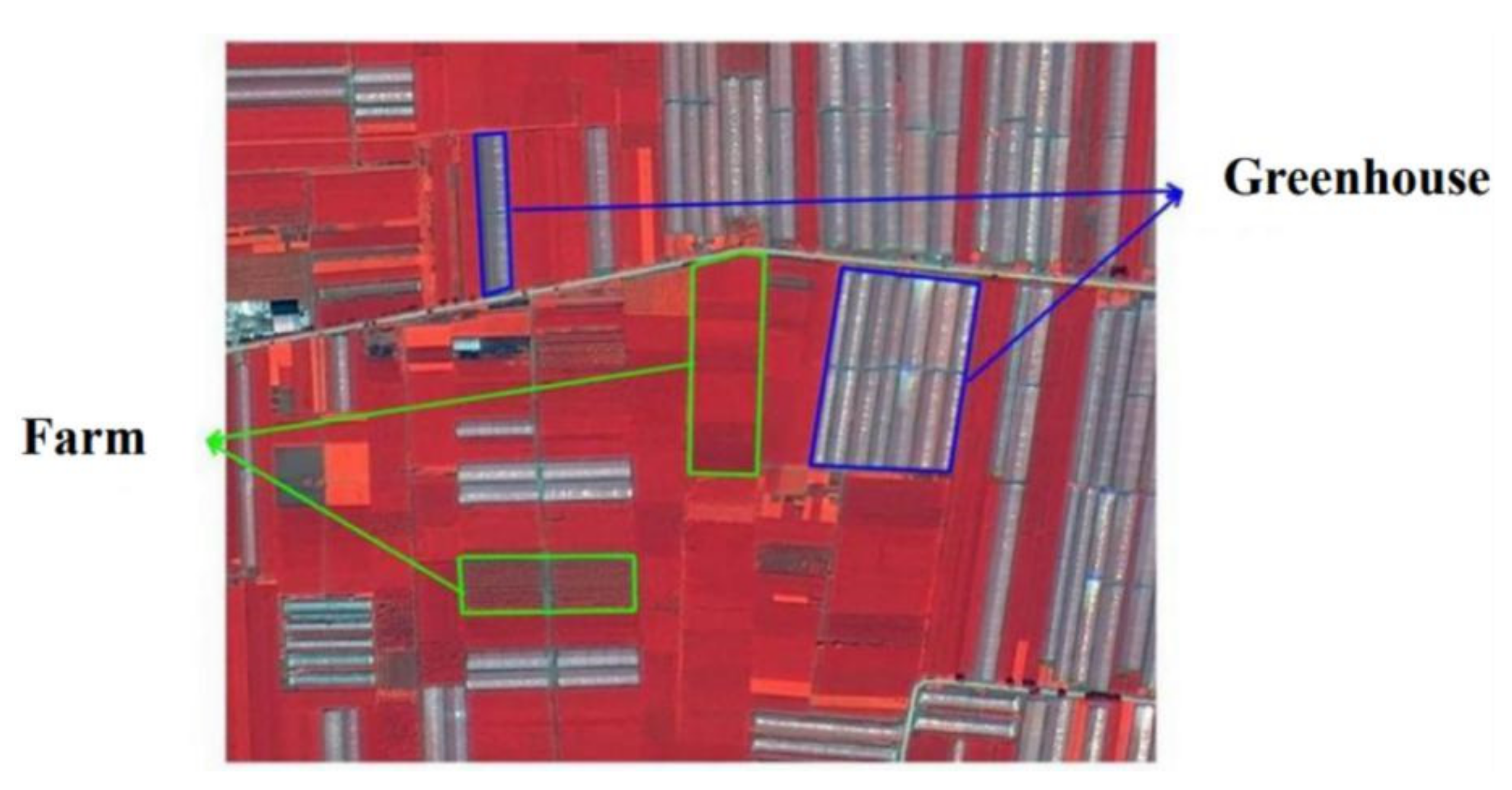
The data source of this study is the Gaofen-2 remote sensing image. Gaofen-2 is the first civil optical remote sensing satellite independently developed by China with a spatial resolution better than 1 m [47]. It is equipped with two imaging devices, a panchromatic camera and a multispectral camera [48]. The specific camera spectral information is shown in Table 1. This study used the remote sensing data of Gaofen-2 in the study area on 16 August 2019. The preprocessing includes radiometric correction, atmospheric correction, and orthorectification. Among them, radiometric and atmospheric correction converts grayscale values to spectral reflectance. In radiometric correction, gain values in four bands are set to be 0.1748, 0.1817, 0.1741, 0.1975 and offset values in four bands are set to be −0.5930, −0.2717, −0.2879, −0.2773. In the process of atmospheric correction, central wavelengths are set to be 514 nm, 546 nm, 656 nm, and 822 nm for the FLAASH model, and the aerosol model is set to be rural in inversion, the single scale factor is set to be 10 for unit conversion of spectral radiance. Orthorectification is used to correct geometric and environmental effects caused by bias. The three processes in preprocessing set pixel size to 0.8 m. The preprocessing is completed using ENVI5.2 (The Environment for Visualizing Images) software. The spatial resolution is 0.81 m, which can clearly and prominently display the morphological characteristics of agricultural greenhouses, as shown in Figure 2. The false color image is synthesized by the near-infrared band, red band and green band, corresponding to the three RGB channels, respectively, which can display the greenhouses more clearly.
After preprocessing the image of the study area, the NDVI [49] (Normalized Difference Vegetation Index) of each pixel of the remote sensing image is calculated by using the band operation, as shown in the following Formula (1):
N D V I = N I R R N I R + R
Among them, NIR represents the near-infrared band, and R represents the red band. The calculated NDVI is used as the fifth band to fuse with the four-band data of the Gaofen-2 remote sensing image to obtain five-band remote sensing image data, which has more abundant spectral data information. In the training of the greenhouse area extraction and quantity estimation model, only the semantic segmentation baseline training of the ENVINet5 [31] framework uses large-scale remote sensing data including five bands, and the remaining model network training only uses images including three optical bands of RGB.

2.3. Greenhouse Dataset

The dataset is cropped from the preprocessed high spatial resolution remote sensing images. The image size of the dataset is set to about 640 × 640 pixels. It is notable that these images only contain the three optical bands, i.e., blue, green, and red. Vegetable and fruit greenhouses are generally square, mainly dark gray and brown. Because the greenhouses are arched, there are obvious protrusions in the middle. The surface of vegetable and fruit greenhouses is mostly made of plastic material, which results in the phenomenon of reflection. The distribution density varies, some of the greenhouses are single and scattered, and some are concentrated and connected together.
The principle of setting the segmentation size [21] is to extract the most suitable feature types for the region. Generally, the smaller the heterogeneity of surface objects in the image, the larger the segmentation size design. Contrarily, become smaller. In the experiment on the picture size in the dataset, it is found that the picture should not be too small or too large. If the area of the vegetable and fruit greenhouses in the figure is too large, the whole picture will be judged as vegetable and fruit greenhouses when the neural network is segmented, resulting in high model training accuracy but a poor image segmentation effect. Therefore, the proportion of 30%~50% can be the most appropriate to identify the greenhouses. The picture should fully contain each agricultural greenhouse, or the labeled data will be broken during labeling, which would cause a lot of noise in the segmentation results.
There are various methods [23,50] for data sample collection, and this is a step that impacts results. We choose to capture 240 high-quality images from the original image, but the number of samples is too small to get a good model accuracy and segmentation effect. Moreover, to avoid overfitting, we maintain the balance of positive and negative samples. We use the method of rotating images to expand the dataset resources. After the images are rotated by 90°, 180°, and 270° for data expansion, 960 images with a varied distribution density of the greenhouses are obtained as original images. They are annotated by ourselves, especially a large number of concentrated greenhouses samples, so the trained model can better extract dense objects. The dataset is divided into a training set and a validation set according to 9:1. The model training uses the pictures of the training set and adjusts the parameters of the neural network convolution kernel and weight by calculating the loss function value to obtain the optimal model.

3. Dual-Task Algorithm

3.1. Dual-Task Learning Module

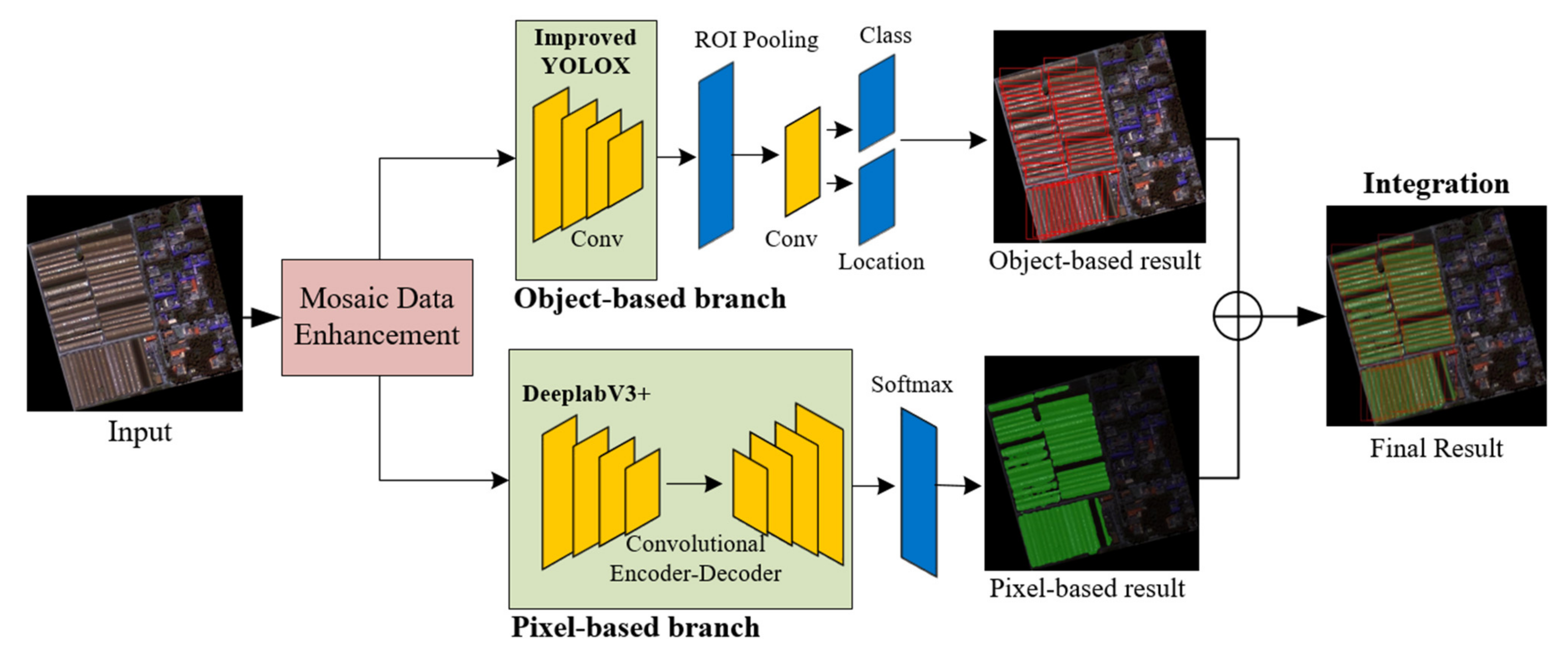
This study proposes a dual-task algorithm (PODD) for area extraction and quantity estimation based on the fusion of the target detection model and semantic segmentation model of agricultural greenhouse detection. The PODD algorithm is illustrated in Figure 3 and is divided into two branches, an object-based branch for quantity extraction and a pixel-based branch for area extraction. In the object-based branch, the lightweight YOLOX network structure is improved, and the attention mechanism and adaptive feature fusion module are embedded in the convolution network feature extraction stage, which improves the detection accuracy and retains more important feature information. In the area extraction of the pixel-based branch, the DeeplabV3+ neural network, whose backbone is replaced by ResNet-101 as the feature extraction network, can effectively reduce the problem of holes and plaques and accurately extract edge information.

3.1.1. Mosaic Data Enhancement

The data expansion of the training dataset and the increase in the number of iterations of the training are conducive to enhancing the generalization of the network, preventing overfitting and improving the detection effect. Data enhancement of datasets is usually performed in a manner similar to natural images, including methods such as rotation, mirror transformation, upside-down flipping, noise augmentation, cropping and padding, and brightness transformation. In this paper, the Mosaic data enhancement module [51] is introduced in the training process to achieve the effect of data enhancement based on manually expanding the dataset. The data enhancement method inserted into the Mosaic module can randomly generate training images. The main idea is to cut four images randomly and then splice them into one image for enhancement. Splicing by random scaling, random clipping and random arrangement is very effective for improving the detection effect of small targets, enriching the image’s background, and the enhanced data can produce a more robust model.

3.1.2. Transfer Learning

Traditional machine learning algorithms must be retrained every time, which takes more time. Because the features extracted from the main feature extraction part of the neural network are common, transfer learning [52] can learn the common features of different similar models. Among them, low-level semantic features such as image shape and color can be extracted by a shallow convolution network, and more abstract and complex deep features can be extracted by a deep convolution layer. Since the convolution layer and the full connection layer at the bottom of the network play a decisive role in different tasks, only the convolution layer before the network model must be frozen when training the new model, and the last few layers of the network need to be retrained. The trained model parameters are migrated to a new sample for further training to obtain the new model.
Before using neural network training, the ImageNet dataset was firstly used for pre-training, and then fine-tunes the parameter on our greenhouse dataset in VOC dataset format [53] to obtain the initial trained network model. Pre-training the neural network with this initial model to learn similar features between datasets can not only train a better model with a small number of training samples but the training process only includes the last few layers of the model with short time and high efficiency.

3.2. Target Detection Network for Greenhouse Quantity Estimation

YOLOX [40] (you only look once) is a regression-based target detection algorithm proposed in 2021, an empirical and experimental improvement of the YOLO series. The development of YOLOX is based on the operation of the PyTorch framework [54]. Multi Positives, decoupling head, Anchor-free mechanism, advanced label allocation strategy, and strong data augmentation are used to construct an innovative high-performance detector. The feature extraction network of YOLOX is composed of multiple sets of residual modules. The activation function is Sigmoid-weighted Linear Unit (SiLU) function [55], which is computed by the sigmoid function multiplied by its input. SiLU is a self-gated activation function and has the characteristics of no bound, smoothness and non-monotonicity. The multi-layer features are fused. Target detection is carried out on feature maps of different sizes, which can detect multiple targets at one time and has high target detection accuracy.
Based on YOLOX lightweight network, CBAM was embedded in the backbone network, and ASFF was added to the feature pyramid to improve the accuracy of target detection on small target datasets.

3.2.1. Feature Attention Mechanism

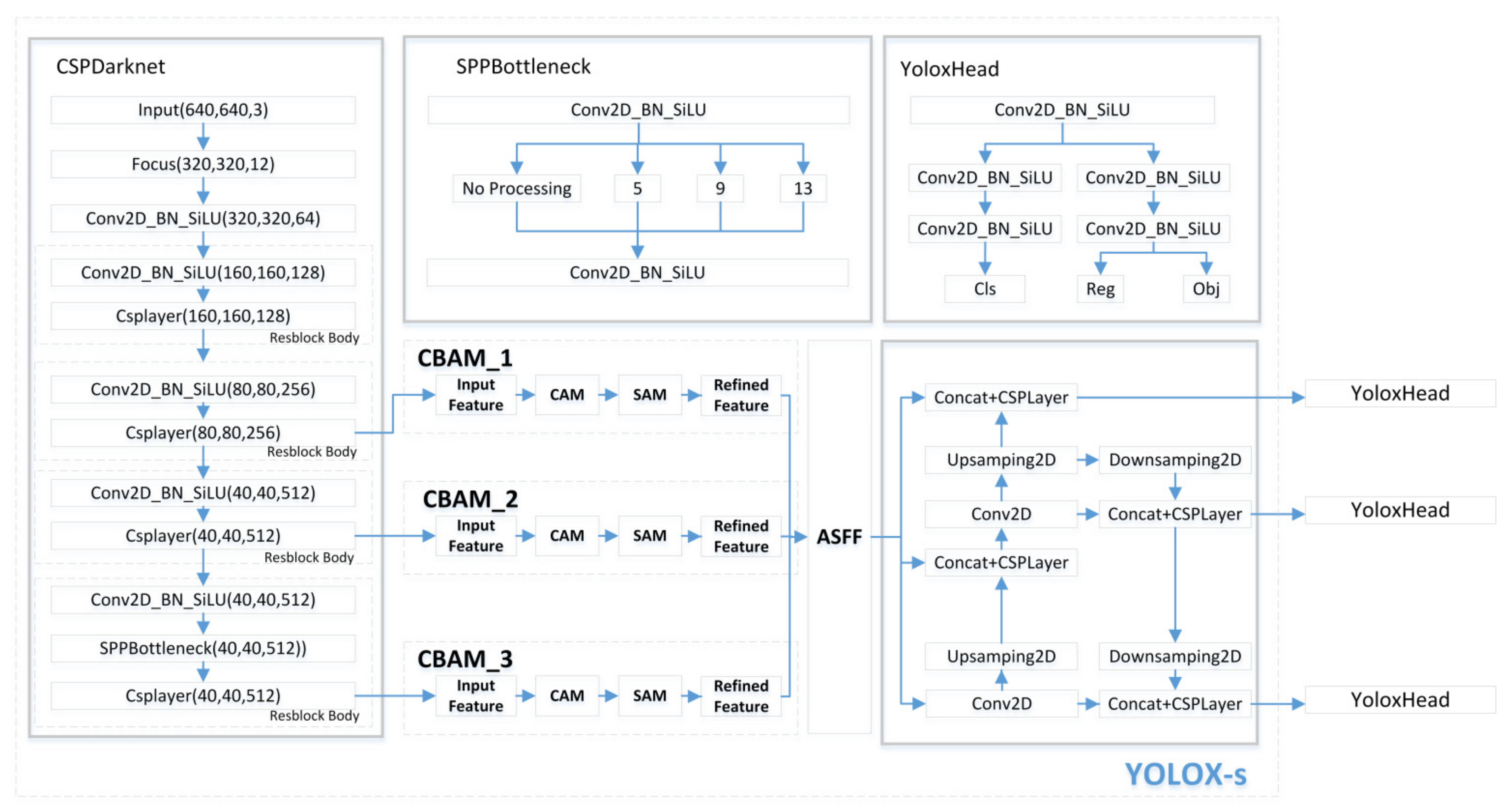
To enhance the feature learning ability of the network, the feature attention mechanism is introduced into the backbone network of YOLOX by inserting CBAM [41]. The insertion position and structure are shown in Figure 4.
The feature attention mechanism selectively extracts a small amount of important information from a large number of information. It focuses on this important information, ignoring most of the less important information. According to the research [56], the introduction of an attention mechanism can make the network pay more attention to the noise area in training, improve the network attention to detail texture, suppress the background, and improve the final denoising effect, to improve the performance of the target in the image. In the target detection task, CBAM includes two independent sub-modules, Channel Attention Module and Spatial Attention Module [57], to conduct attention concentration operations on channel and space, respectively. This ensures that CBAM can not only be fully integrated into the existing network architecture but also save the parameters and computing power in the training process and improve the accuracy of target detection training results. The implementation steps of CBAM are as follows: firstly, the weighted results are obtained by the convolution layer output information through a channel attention module; then, the final result is weighted by a spatial attention module.
The channel attention mechanism is to compress the feature map in the spatial dimension through average pooling and maximum pooling to obtain a one-dimensional vector. The average pooling and maximum pooling can aggregate the spatial information of feature maps for delivery to a shared network, compress the spatial dimensions of the input feature maps, and merge element-wise sums to generate channel attention maps. The average pooling feedback is for each pixel on the feature map, while maximum pooling only performs gradient feedback on the position with the largest response in the feature map during the gradient back-propagation calculation. Channel attention mechanism can be expressed as Formula (2) [41]:
M C F = σ ( M L P ( A v g P o o l ( F ) ) + M L P M a x P o o l F ) = σ ( W 1 W 0 F A v g c   W 1 W 0 F m a x c )
where AvgPool denotes the average pooling operation, MaxPool represents the maximum pooling operation, σ represents the sigmoid operation, and W0 and W1 are the weight values of the MLP on the input features.
The spatial attention mechanism compresses channel dimensions through average pooling and maximum pooling. The maximum pooling operation is to extract the maximum value on the channel, and the number of extraction times is height multiplied by width. The average pooling operation is to extract the average value on the channel, and the number of times of extractions is height multiplied by width. Then the feature maps with the channel number of 1 are merged to obtain a feature map with the channel number of 2. The spatial attention mechanism can be expressed as Formula (3) [41]:
M C F = σ f 7 × 7 A v g P o o l F ; M a x P o o l F = σ f 7 × 7 F a v g s ; F m a x s
where f 7 × 7 represents the convolution operation, 7×7 represents the size of the convolution kernel, and the convolution kernel of 7×7 is better than that of 3×3 [41].

3.2.2. Adaptive Spatial Feature Fusion

To make full use of the semantic information of high-level features and the fine-grained features of low-level features, ASFF [43] module is added to the feature pyramid to fuse the features in a weighted way, as the insertion position is shown in Figure 4. Figure 5 describes the specific process of feature fusion, which can be separated into two steps, identically rescaling and adaptively fusing. For each level, the features of all the other levels are resized to the same shape and spatially fused according to the learned weight maps. The weighted fusion process of fusing the features at the corresponding level l is shown in Formula (4):
y i j l = α i j l · x i j 1 l + β i l l · x i j 2 l + γ i j l · x i j 3 l  
Among them, xn→lij denotes the feature vector at the position (i, j) on the feature maps resized from level n to level l. The features from different layers are multiplied by the weight parameters α, β and γ, respectively, to obtain a new fusion feature. Due to the addition method, the output features of level 1~3 layers must be the same size and the same number of channels. The number of channels should be adjusted after up-sampling or down-sampling the features of different layers. The weight parameters α, β and γ are obtained by adjusting the image size, and then the feature map of level 1 to level 3 is obtained by 1 × 1 convolution layers, respectively. After connection, the normalized exponential function softmax is used to make the range in [0, 1], and the sum is 1; Formula (5) [43] is as follows:
α i j l = e λ α i j l e λ α i j l + e λ β i j l + e λ γ i j l
Here αlij, βlij and γlij are defined by using the softmax function with λlαij, λlβij and λlγij as control parameters, respectively. The weight scalar maps λlα, λlβ and λlγ are computed from x1→l, x2→l and x3→l respectively, by 1 × 1 convolution layers through standard back-propagation.

3.3. Semantic Segmentation Network for Greenhouse Area Extraction

After the data enhancement, on the one hand, it enters the target detection network to estimate the quantity of greenhouses. On the other hand, it enters the semantic segmentation network to extract the greenhouse area. For the extraction algorithm of greenhouse area, this work focuses on the semantic segmentation algorithm of the Deeplabv3+ neural network.
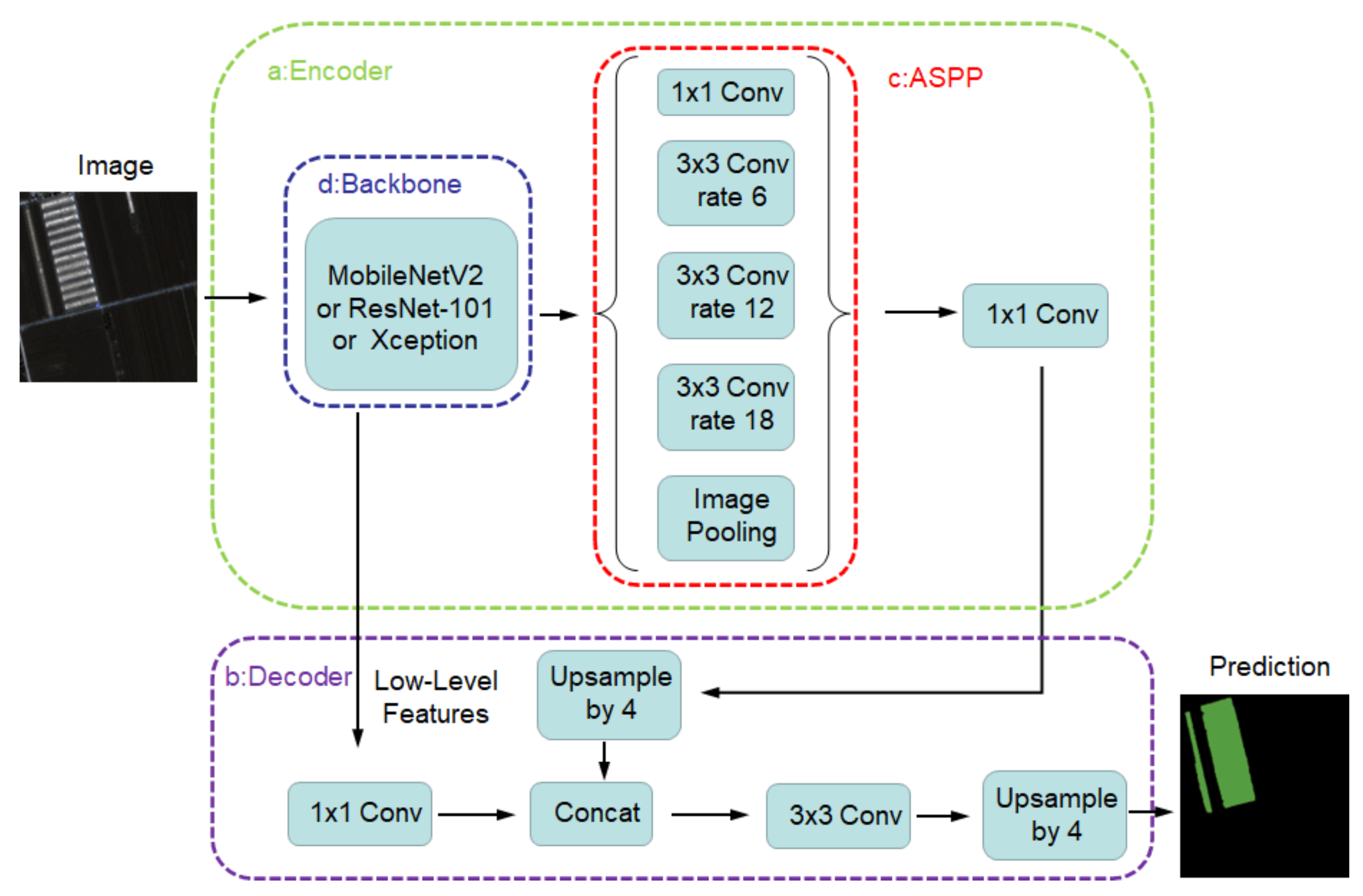
Deeplabv3+ [43,44,45] is the fourth-generation deep-learning network structure of the Deeplab series proposed by Google in 2018. It uses DeepLabv3 neural network as the encoding model [58], which mainly includes a backbone network and atrous spatial pyramid pooling (ASPP) module, and its network structure is shown in Figure 6. To obtain high-resolution features, the encoder–decoder structure combines the features of different levels to gradually obtain relatively fine features, where the Encoder is the downsampling module responsible for feature extraction, and the Decoder is the upsampling module (through interpolation, transposed convolution, etc.) responsible for restoring the size of the feature map. The encoding introduces atrous convolution to extract multiscale context information, the low-level features extracted by the backbone are used as boundary information, and the high-level features extracted by ASPP are used as semantic information. The boundary information and the up-sampled semantic information are fused and concatenated in the decoder to obtain the final extracted features. Since no feature extension is used, the encoding structure can extract dense features more quickly under the same calculation conditions and gradually restore clearer boundary information in the decoder. The introduction of atrous convolution can predict the calculation resources and control the density of encoder characteristics to obtain more detailed object boundary information.
The backbone network of DeeplabV3+ is one of the encoding components, which is responsible for feature extraction from the input training data, providing low-dimensional features and input features for the decoding model and the ASPP structure, respectively. The backbone network can use feature extraction networks such as MobileNetV2 [59], ResNet [46] or Xception [60]. Neural networks of different structures and complexity will affect the training speed and accuracy. The DeeplabV3+ model widely uses optimized Aligned Xception [60] or MobileNetV2 [59] as the backbone network for training. The optimized Aligned Xception model can obtain a variety of resolution features, which is based on the Inception series network structure combined with depthwise separable convolution. Xception splits the Inception model into a series of operations to become simpler and more efficient and deals with spatial and cross-channel correlations independently. MobileNetV2 [59] is a lightweight neural network designed for mobile scenarios and resource-constrained environments based on MobileNetV1 [61]. MobileNetV2 uses a depthwise separable convolution and residual structure and introduces the idea of inverted residuals, which significantly reduces the number of parameters of the neural network. At the same time, the RELU6 activation function is used to make the model more robust under low-precision calculations. ResNet [46] uses a deep residual network to solve the problem that the accuracy of the training set decreases due to the deepening of the neural network not caused by overfitting, so that increasing the depth of the neural network can significantly improve segmentation accuracy. ResNet-101 is a deeper structure of ResNet, which contains a total of 101 convolutional layers and fully connected layers: 1 7 × 7 convolutional layers, 33 Building Blocks with a total of 99 layers, and 1 fully connected layer.

3.4. Integration for Greenhouse Area Extraction and Quantity Estimation

Section 3.2 and Section 3.3 introduce a target detection network for greenhouse quantity estimation and a semantic segmentation network for greenhouse area extraction, respectively. The extraction processes of the two independent branches end with object-based and pixel-based results consequently. To quantify the development status of greenhouses in the region from two dimensions of area and quantity, remote sensing images for object-based image results and pixel-based image results are integrated to achieve the final image result with both area extraction and quantity estimation based on image fusion technology. The integration between object-based and pixel-based image results makes up for spatial distribution errors caused by a single result visually. At the same time, the integration of image results and the combination of quantitative results can complement each other and support each other visually and numerically.

4. Experimental Results

Based on remote sensing images of Wugong Town, Raoyang County, Hengshui City, the quantity and area of greenhouses are extracted. Before the experiment process, the original image is cropped to a smaller size before it can be input into the model, so the entire panorama is cropped. Then, the image size is normalized to 640 × 640 image resolution to reduce the amount of network operations, and it is used as a data set for model training. In this experiment, the computer is configured with one NVIDIA GeForce RTX 3060 (6 G) Laptop GPU and a total memory of 32 G.

4.1. Evaluation Metrics

After the optimal model is obtained by neural network training, the accuracy is evaluated using the validation dataset that is not trained. To quantitatively evaluate results, objects (or pixels) are sorted into true positive (TP), true negative (TN), false positive (FP), and false negative (FN) based on ground truth labels.
As for object detection, IoU is the ratio of intersection and union of the prediction box and ground truth. Then, according to the IoU threshold, when the category of an object is determined correctly, the confidence level is high enough, and the intersection over union (IoU) between the detection box and labeled reference box reaches a certain threshold, it is considered that the prediction is correct.
I o U = A r e a A B A r e a A B  
Among them, A represents the prediction box, B is the benchmark box, and Area denotes the area operation after calculating the number of True Positives (TP) and the number of False Positives (FP).
The precision of each category can be calculated by Formula (7). Recall is the proportion of all positive samples in the test set that are correctly identified as positive samples. F1 evaluates the model’s accuracy by F1-score based on the consistency of the importance of recall and precision. The evaluation index commonly used to describe the classifier is the mean Average Precision (mAP), which is the average accuracy rate of each category.
P r e c i s i o n = T P T P + F P  
R e c a l l = T P T P + F N  
F 1 = 2 1 Recall + 1 Precision
As for Semantic segmentation, the accuracy of the model is evaluated by using the Accuracy rate (Acc) and the mean Intersection-over-Union (mIoU). Acc is the ratio of the correct number of pixels in the validation set image to the total number of pixels. mIoU (Mean Intersection over Union) is the weighted average of IoU, calculated as (k represents the number of classes):
A c c = T P + T N T P + T N + F P + F N  
m I o U = 1 K + 1 0 K T P F N + F P + T P  

4.2. Estimation of Greenhouse Quantity

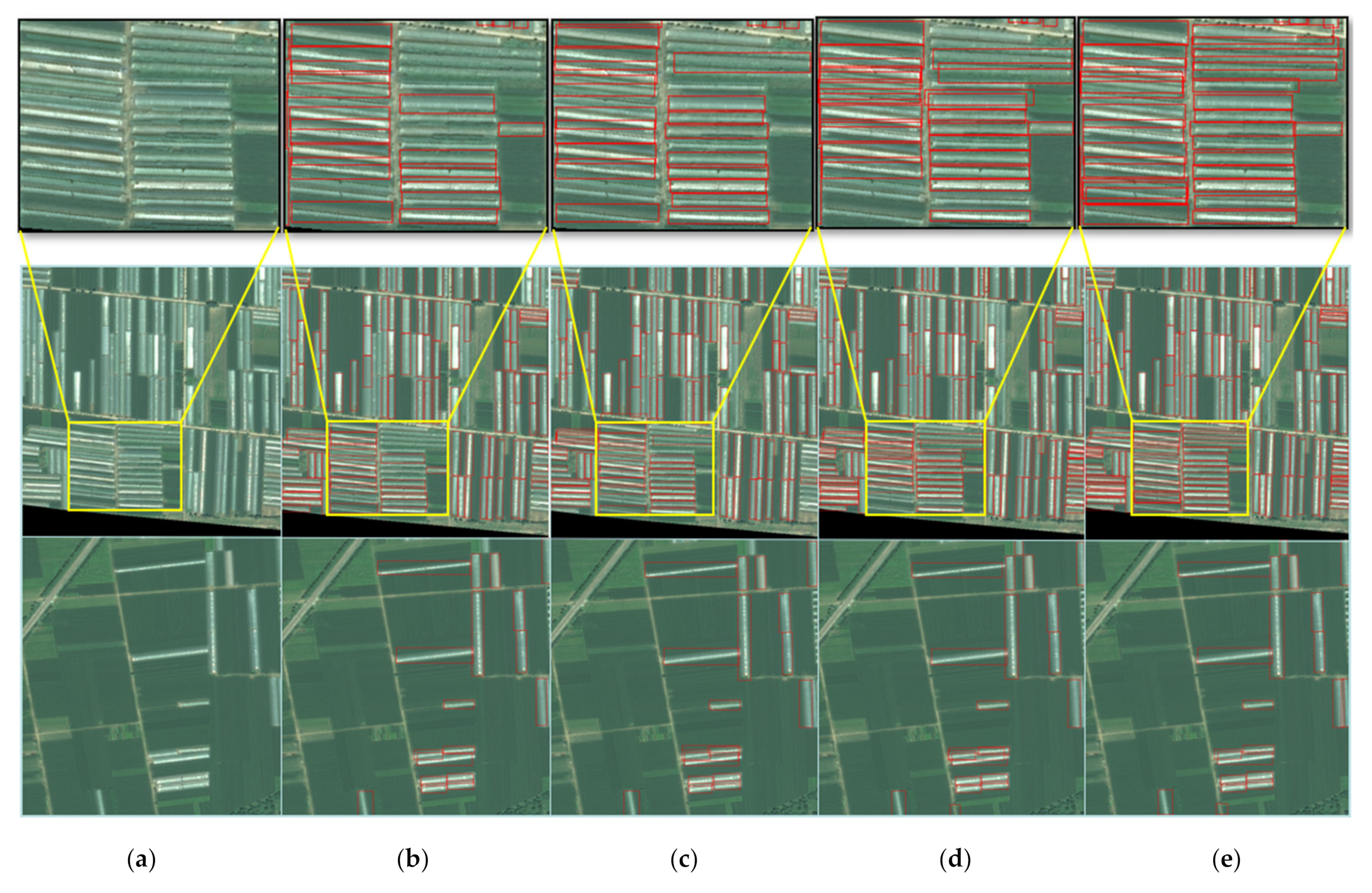
In this paper, the dataset is trained with an improved YOLOX model using the PyTorch framework, and 864 sheets are randomly selected as the training set and the remaining 96 sheets as the test set. Before using neural network training, the neural network is first transferred to the neural network using the YOLOX model trained on the ImageNet dataset. The results of the greenhouse extraction of the centralized distribution (the first line) and the dispersed distribution (the second line) using the improved YOLOX model before and after are shown in Figure 7.
Through the comparative observation of the target’s detection effect of the greenhouse of lightweight YOLOX neural network and various improved network models, in the case of scattered greenhouse distribution, various methods can accurately detect the location and quantity of basic greenhouses. However, in the case of very dense greenhouse distribution, many greenhouses are concentrated into blocks, and there are a small number of missed targets in the target detection process in a lightweight YOLOX network. As we can see from the concentrated distribution condition especially shown in enlarged fragments, there are obvious incremental improvements in the detection from column (b) to column (e). Above all, the improved YOLOX network embedded in CBAM and ASFF has a more accurate detection effect on the concentrated distribution. The error of missed detection targets is significantly reduced.
With an IoU threshold of 0.65 and a confidence threshold of 0.7, the detection results of the greenhouse quantity of YOLOV5 [62] and different YOLOX improvement methods are shown in Table 2. It can be seen that YOLOX has a better performance than YOLO5 through metrics due to the improvements in data augmentation, anchor-free algorithm, SimOTA label assignment, and so on in the YOLOX structure. The detection accuracy of the improved YOLOX network is better than the original YOLOX network. The insertion of CBAM in the YOLOX network structure can make up for the lack of expression ability of its feature extraction layer, and the addition of the ASFF module can make full use of the features of different scales. The combination is more robust than other ways on each accuracy metric, improving the accuracy of the model. YOLOX optimal model embedded CBAM and ASFF modules were finally selected to detect the greenhouses in the study area, and the results were obtained as a total of 5827 greenhouses.

4.3. Extraction for Greenhouse Area

4.3.1. Evaluation of DeeplabV3+ Models with Different Backbone Networks

The performance of DeeplabV3+ models with different backbone networks, such as the optimized Aligned Xception model, MobileNetV2 and ResNet-101 neural networks, are compared through experiments, and the most suitable model for semantic segmentation of greenhouses is selected as the backbone network. Firstly, the neural network is pre-trained using the MobileNetV2, ResNet-101 and Xception models trained on the ImageNet dataset. Before the fully connected layer, the ratio of the input image resolution to the output feature resolution of the encoding structure is set to 16, 8, and 16, respectively. The initial learning rate of the freezing stage is 1 × 10⁻³, the initial learning rate of the thawing stage is 1 × 10⁻⁴, and the total number of trainings is 43,200 times. Then the weight file is obtained and the learning rate is reduced to 1 × 10⁻⁵.
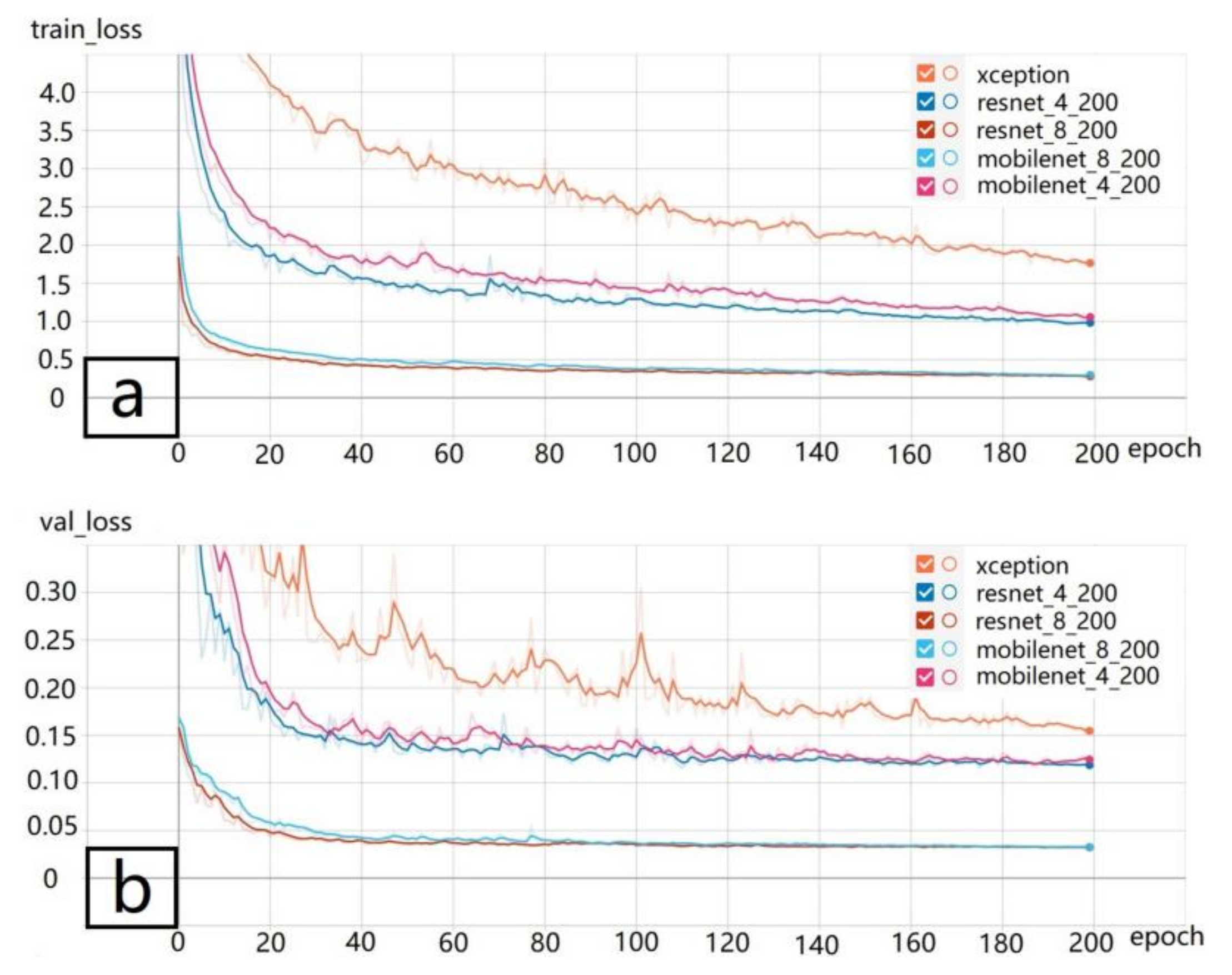
By adjusting the backbone and batch-size parameters, five groups of neural network types are set. Figure 8a,b show the changing trend of the loss function of the training dataset and the validation dataset of the 5 groups of neural network types during training, respectively. The 5 groups of neural network models increase with the number of trainings, the loss function value decreases significantly in the early stage, tends to be flat in the later stage, and is basically stable after reaching a certain small value. The ResNet-101neural network with a batch size of 8 performed best, followed by the MobileNetV2 neural network, whose loss function curve fell fast and smoothly. While the optimized Aligned Xception neural network performed poorly, the two curves changed slowly, the curve volatility was large, and the loss function value of the verification set was significantly higher than that of the other groups of neural networks.
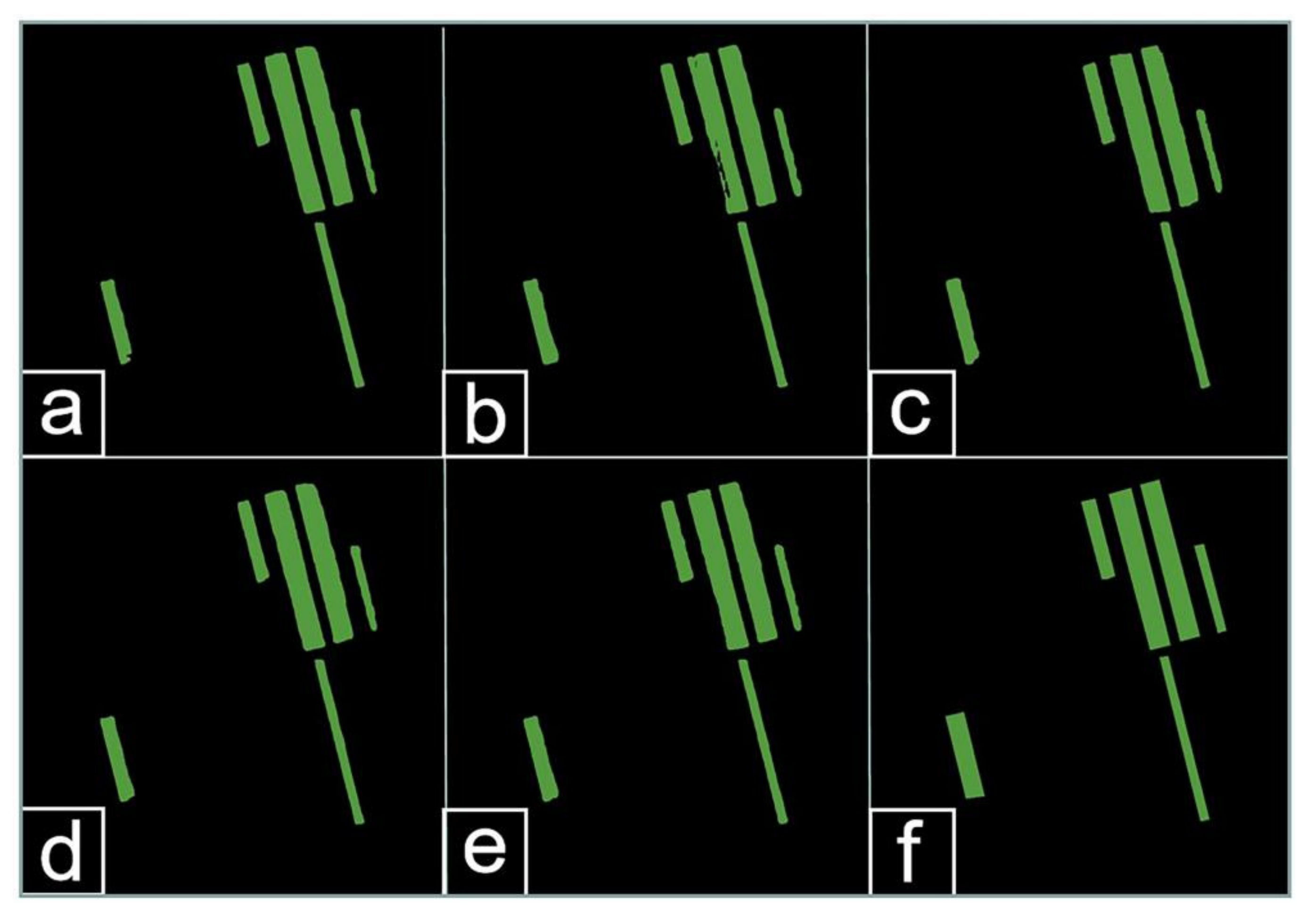
The greenhouse segmentation results of the DeeplabV3+ model with different backbone networks are shown in Figure 9. It can be seen that the ResNet-101 neural network with a parameter batch size of 8 (ResNet_8_200) performs best, and there is no void or plaque. The DeeplabV3+ neural network, whose backbone is replaced by ResNet-101 as the feature extraction network, can effectively reduce the problem of holes and plaques and accurately extract edge information. The other four groups have incomplete extraction, and a small part of the edges are missing; increasing the parameter batch size can significantly improve the integrity and regularity of the greenhouse segmentation. Comparative testing of the DeeplabV3+ models with five groups of backbone neural networks with specific parameters is shown in Table 3. By comparing the evaluation metrics on accuracy, mIoU, and training time of validation set semantic segmentation, the optimal model trained ResNet_8_200 with the best performance is finally selected to segment the greenhouse in the study area.

4.3.2. Comparative Test of Different Network Structures

The three semantic segmentation models, the DeeplabV3+ model, ENVINet5 framework [31], and UNet [26], were conducted to perform a comparative test. The greenhouses in Wugong Town, Hengshui City, Hebei Province, is the study area with the spatial resolution of the high-resolution data of 0.81m. The results of the segmented global map of greenhouse area extraction by the DeeplabV3+ model, ENVINet5 framework and UNet are shown in Figure 10. It is clear that the DeeplabV3+ model can yield the best performance, as we can see from the enlarged fragments.
The accuracy metrics of three different network structures are analyzed and compared in the following Table 4. It is clear that the DeeplabV3+ network model performs better than ENVINet5 and UNet in terms of both accuracy and mIoU. The result of the DeeplabV3+ network can also be observed on the local segmentation graph that can effectively reduce cavitation and plaque problems, so the DeeplabV3+ network model is more applicable and more accurate in the application of greenhouse area extraction.
The greenhouse area of Wugong Town is calculated by the method of pixel statistics, and the result of the DeeplabV3+ model to segment the greenhouse, the result is 8,148,531.77 square meters, totaling 302.021 acres.

4.4. Integration for Greenhouse Area Extraction and Quantity Estimation

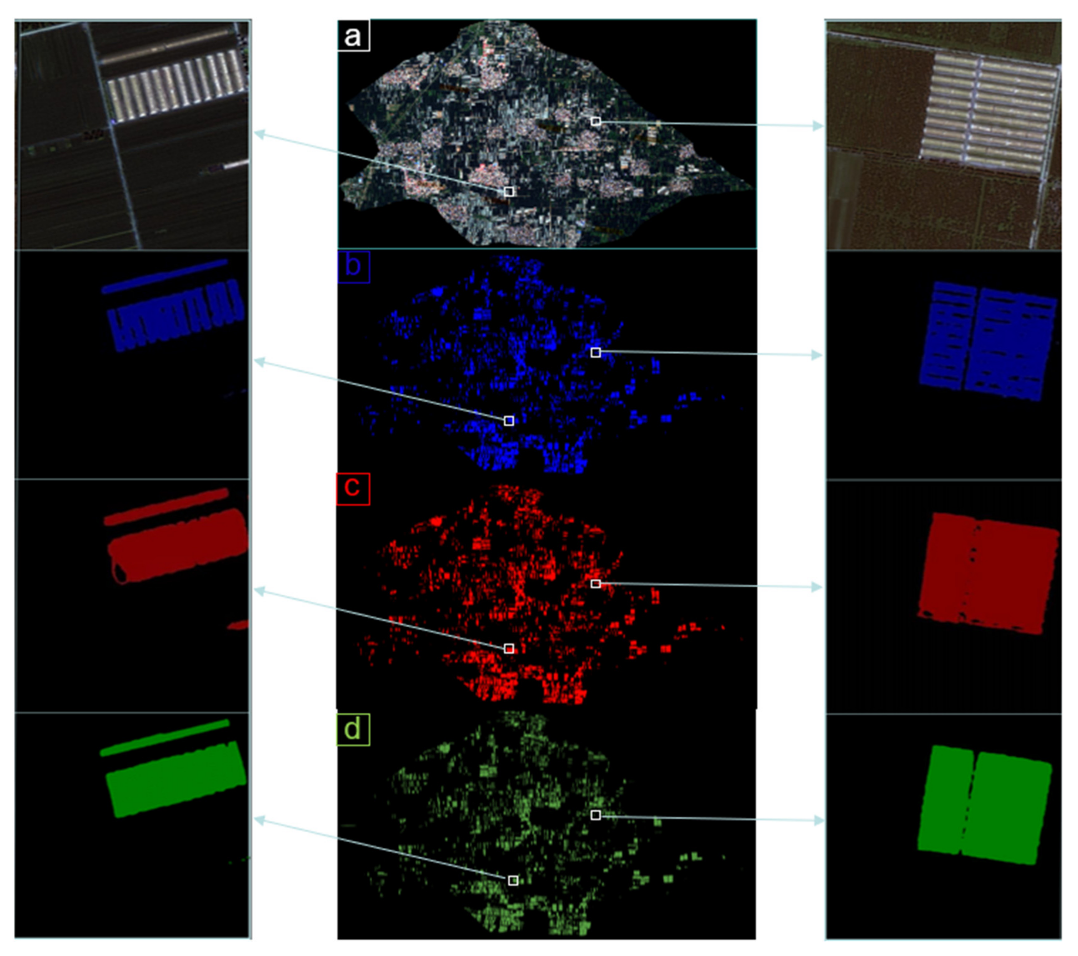
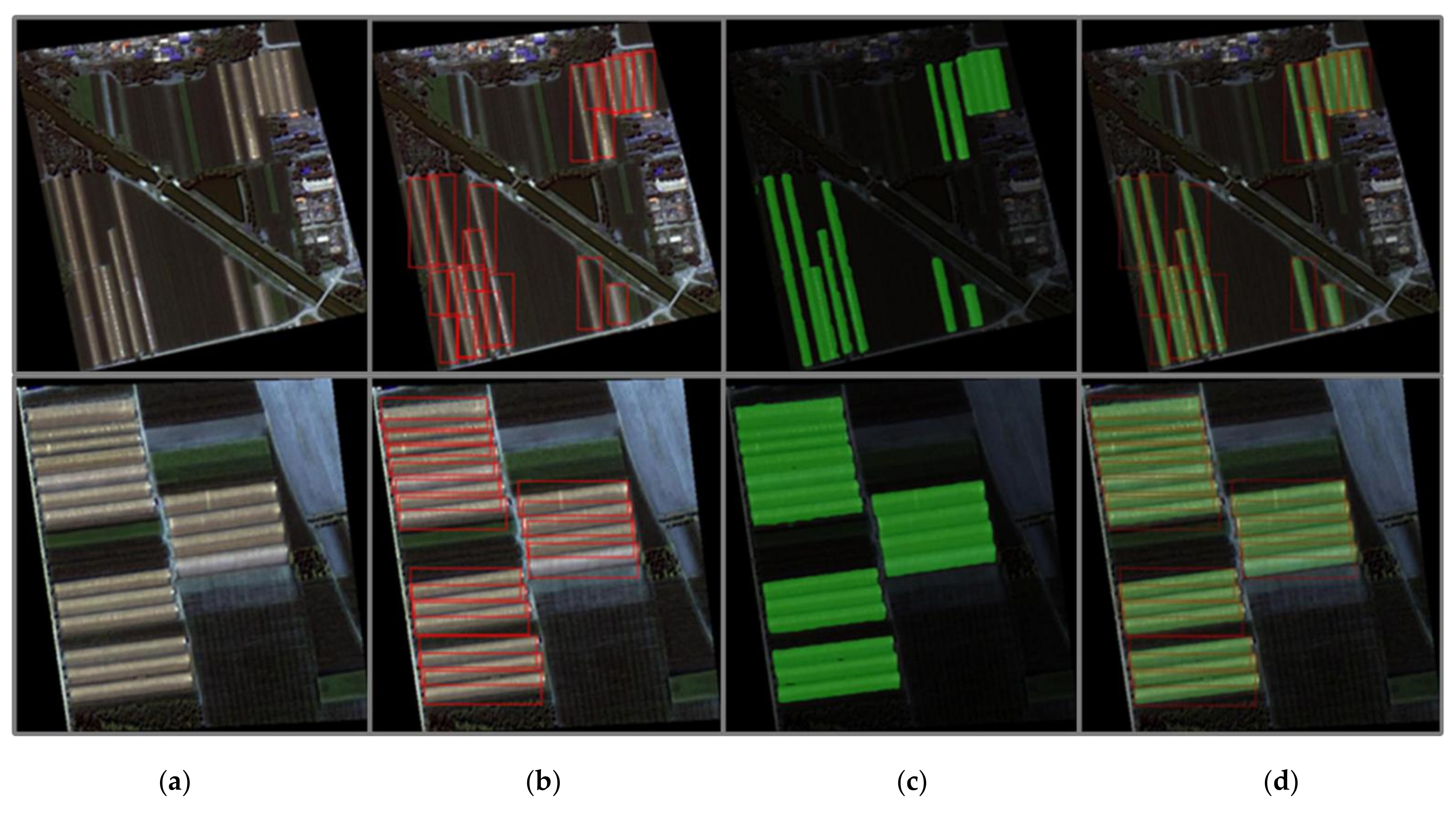
Aiming at quantifying the development status of greenhouses in the region from two dimensions of area and quantity, remote sensing images for object-based image results and pixel-based image results are integrated to achieve the final image result with both area extraction and quantity estimation based on image fusion technology visually. The proposed was used to extract the greenhouse in two cases of scattered distribution (the first line) and centralized distribution (the second line), and the results are shown in Figure 11. The combination of target detection and semantic segmentation can detect the spatial distribution of greenhouses accurately and effectively in both cases.

5. Discussion

5.1. Advantages of PODD Algorithms

As a special kind of surface object, extraction and detection of greenhouses are crucial in agriculture and environmental management. There have already been some researches focusing on the extraction of greenhouses from remote sensing images [63]. Among these researches, the spectral index method by constructing new indices or index combinations is the most popular. For example, Yang et al. [8] proposed a new spectral index (RPGI) for greenhouse extraction from high-resolution remote sensing images. Shi et al. [64] suggested using a series of spectral indices to separate greenhouse pixels from the neighboring environment to the maximum extent. However, the spectral index method is a kind of pixel-based method without considering the property of the greenhouse as a whole object. Furthermore, the spectral index method is useful in medium-resolution remote sensing images with relatively high accuracy when greenhouses occupy more than 12% of the pixel. However, the characteristics of greenhouse covering film lead to the complexity of the spectral characteristics of ground objects; the spectral index method is unsuitable for high-resolution remote sensing due to the complex spectral characteristics of the greenhouse surface. This seriously confuses plastic greenhouses with other land types (construction land, roads, unused land). Therefore, the traditional machine learning-based method is also widely used in greenhouse extraction [65]. It, combined with the characteristics of spectral index, texture and shape, is robust to the spectral differences which stem from the different materials of greenhouses. However, the traditional machine learning-based method can only extract hand-crafted features, which may be ineffective in real application scenes [66]. Hand-crafted geometric features are unable to distinguish greenhouses and buildings. At the same time, greenhouses vary greatly in different regions and seasons, and traditional methods have poor generalization ability in complex scenes [67]. In addition, the algorithms mentioned above all play a role in one dimension of greenhouse extraction, which can only obtain the quantified information of the greenhouse area with different accuracy. However, the researches related to estimating greenhouse quantity based on object detection remain few and are also taken alone.
Considering the above problems, in this study, we proposed a novel method, PODD, which combines object detection (quantity estimation) and semantic segmentation (area extraction). The PODD algorithm utilizes deep learning algorithms. It could treat greenhouses as objects and captures their morphological characteristics, and could extract the area distribution accurately with a better generalization ability than traditional methods [36,68]. The parameters, such as the confidence threshold, the IOU threshold, training epoches, and batch size we set play a very significant role in the effect of our proposed algorithm, so many trials and experiments with different parameters are implemented to maximize the accuracy and precision and compress the training time to optimize the final effect. With the PODD algorithm, quantity and area could be extracted with high accuracy. In this study, GF-2 data is used to validate the PODD algorithm. The experiment results demonstrate that PODD can accurately extract both area and quantity (>95%), indicating that the proposed enhancement approach is useful in agricultural greenhouse extraction. The integration between object-based and pixel-based image results makes up for spatial distribution errors caused by a single result visually. At the same time, the integration of image results and the combination of quantitative results can complement each other and support each other visually and numerically. Generally, the combination can accurately quantify the development status of greenhouses in the region from two dimensions of area and quantity, which is of great significance in food demand prediction, greenhouse environmental pollution monitoring and agricultural planting planning.

5.2. Limitations and Further Perspectives

Although our proposed PODD algorithm could extract both the quantity and area of greenhouses in remote sensing images, there are still some limitations in this algorithm. Firstly, the concentrated greenhouses with very small distances from each other could not be separated accurately, which will decrease the number of greenhouses and bring some errors in quantity estimation. Secondly, the optical properties of greenhouses also limit the area extraction accuracy as the optical properties of greenhouses are very different, mainly determined by the vegetation planted inside the greenhouses. Therefore, more sample datasets for greenhouses are also needed to train a more accurate deep-learning model for greenhouse extraction. Thirdly, our research of extracting greenhouses was taken for the situation only in August when the adopted remote sensing images were photoed, so at other times or seasons in a year, the greenhouses may perform different features, especially when snow covers the greenhouses in winter, so whether our methods can apply to various situation or not needs more validations to test and inspect. Finally, the different spectral characteristics and spatial resolution of remote sensing sensors will also bring some disturbance in greenhouse extractions. Therefore, a universal model suitable for most of the remote-sensing images is necessary for large-scale applications.

6. Conclusions

A Dual-Task Algorithm for Agricultural Greenhouse Extraction Based on Deep Learning (PODD) has been proposed to extract the area and quantity distributions of greenhouses in an agricultural region in north China. The lightweight YOLOX network was improved by inserting CBAM and ASFF modules to estimate the number of greenhouses. Regarding greenhouse area extraction based on DeeplabV3+, Resnet-101 was used as the backbone network to extract greenhouse area through semantic segmentation, which can effectively reduce the problem of void and plaque and accurately extract edge information. The experimental results based on the self-built dataset on greenhouse extraction in a specific region in China achieve peak accuracy value both on the estimation of quantity and area of greenhouses. This algorithm could be used in agricultural production and environmental management for those regions with facility agriculture.

Author Contributions

Conceptualization, F.Y. and W.C.; Data curation, F.Y., J.H., M.W. and M.T.; Funding acquisition, D.W., F.Y. and W.C.; Methodology, J.F.; Project administration, D.W.; Supervision, F.Y. and W.C.; Validation, F.Y., J.H., M.T. and W.C.; Writing—original draft, J.F.; Writing—review & editing, J.F. All authors have read and agreed to the published version of the manuscript.

Funding

This research is funded by the National Key R&D Program of China, grant number 2021YFF0704400; the Undergraduate Training Program for Innovation and Entrepreneurship of CUMTB, grant number 202102010; National Science Foundation of China, grant number 41501416.

Conflicts of Interest

The authors declare they have no known competing financial interest or personal relationships that could have appeared to influence the work reported in this paper.

References

  1. He, W.Q.; Yan, C.R.; Liu, S.; Chang, R.; Wang, X.; Cao, S.; Liu, Q. The use of plastic mulch film in typical cotton planting regions and the associated environmental pollution. J. Agro-Environ. Sci. 2009, 28, 1618–1622. [Google Scholar]
  2. Sun, S.; Li, J.M.; Ma, Y.B.; Zhao, H.W. Accumulation of heavy metals in soil and vegetables of greenhouses in Hebei Province, China. J. Agric. Resour. Environ. 2019, 36, 236–244. [Google Scholar]
  3. Ren, C.; Sun, H.W.; Zhang, P.; Zhang, K. Pollution characteristics of soil phthalate esters in Beijing-Tianjin-Hebei Region. In Proceedings of the 19th Conference of Soil Environment Professional Committee of Chinese Soil Society and the 2nd Symposium of Soil Pollution Prevention and Control and Remediation Technology in Shandong Province, Jinan, China, 18 August 2017. [Google Scholar]
  4. Li, J.; Zhao, G.X.; Li, T.; Yue, Y.D. Information on greenhouse vegetable fields in TM images Technology research. J. Soil Water Conserv. 2004, 18, 126–129. [Google Scholar]
  5. Aguera, F.; Liu, J.G. Automatic greenhouse delineation from QuickBird and Ikonos satellite images. Comput. Electron. Agric. 2009, 6, 191–200. [Google Scholar] [CrossRef]
  6. Aguera, F.; Aguilar, M.A.; Aguilar, F.J. Detecting greenhouse changes from QuickBird imagery on the mediterranean coast. Int. J. Remote Sens. 2006, 27, 4751–4767. [Google Scholar] [CrossRef] [Green Version]
  7. Aguera, F.; Aguilar, M.A.; Aguilar, F.J. Using texture analysis to improve per-pixel classification of very high-resolution images for mapping plastic greenhouses. ISPRS J. Photogramm. Remote Sens. 2008, 63, 635–646. [Google Scholar] [CrossRef]
  8. Yang, D.; Chen, J.; Zhou, Y.; Chen, X.; Chen, X.; Cao, X. Mapping plastic greenhouse with medium spatial resolution satellite data: Development of a new spectral index. ISPRS J. Photogramm. Remote Sens. 2017, 128, 47–60. [Google Scholar] [CrossRef]
  9. Chen, J.; Shen, R.P.; Li, B.L.; Ti, C.; Yan, X.; Zhou, M.; Wang, S. The development of plastic greenhouse index based on Logistic regression analysis. Remote Sens. Land Resour. 2019, 31, 43–50. [Google Scholar]
  10. Liu, T.Y.; Zhao, Z.; Shi, T.G. An Extraction Method of Plastic Greenhouse Based on Sentinel-2. Agric. Eng. 2021, 11, 91–98. [Google Scholar]
  11. Wang, Z.; Zhang, Q.; Qian, J.; Xiao, X. Research on remote sensing detection of greenhouses based on enhanced water body index—Taking Jiangmen area of Guangdong as an example. Integr. Technol. 2017, 6, 11–21. [Google Scholar]
  12. Balcik, F.B.; Senel, G.; Goksel, C. Greenhouse mapping using object-based classification and Sentinel-2 satellite imagery. In Proceedings of the 2019 8th International Conference on Agro-Geoinformatics (Agro-Geoinformatics), Istanbul, Turkey, 16–19 July 2019; pp. 1–5. [Google Scholar]
  13. Novelli, A.; Tarantino, E. Combining ad hoc spectral indices based on LANDSAT-8 OLI/TIRS sensor data for the detection of plastic cover vineyard. Remote Sens. Lett. 2015, 12, 933–941. [Google Scholar] [CrossRef]
  14. Wu, J.Y.; Liu, X.L.; Bai, Y.C.; Shi, Z.T.; Fu, Z. Recognition of plastic greenhouses based on GF-2 data combined with multi-texture features. J. Agric. Eng. 2019, 35, 173–183. [Google Scholar]
  15. Gao, M.J.; Jiang, Q.N.; Zhao, Y.Y.; Yang, W.; Shi, M. Comparison of plastic greenhouse extraction methods based on GF-2 remote sensing images. J. China Agric. Univ. 2018, 23, 125–134. [Google Scholar]
  16. Zhu, D.H.; Liu, Y.M.; Feng, Q.L.; Ou, C.; Guo, H.; Liu, J. Spatial-temporal Dynamic Changes of Agricultural Greenhouses in Shandong Province in Recent 30 Years Based on Google Earth Engine. J. Agric. Mach. 2020, 51, 8. [Google Scholar]
  17. Ma, H.R.; Luo, Z.Q.; Chen, P.T.; Guan, B. Extraction of agricultural greenhouse based on high-resolution remote sensing images and machine learning. Hubei Agric. Sci. 2020, 59, 199–202. [Google Scholar]
  18. Balcik, F.B.; Senel, G.; Goksel, C. Object-Based Classification of Greenhouses Using Sentinel-2 MSI and SPOT-7 Images: A Case Study from Anamur (Mersin), Turkey. IEEE J. Sel. Top. Appl. Earth Obs. Remote Sens. 2020, 13, 2769–2777. [Google Scholar] [CrossRef]
  19. Zhao, L.; Ren, H.Y.; Yang, L.S. Retrieval of Agriculture Greenhouse based on GF-2 Remote Sensing Images. Remote Sens. Technol. Appl. 2019, 34, 677–684. [Google Scholar]
  20. Li, Q.X. Extraction and analysis of agricultural greenhouse area based on high-resolution remote sensing data-taking Daxing District, Beijing as an example. Beijing Water 2016, 6, 14–17. [Google Scholar]
  21. Zhou, J.; Fan, X.W.; Liu, Y.H. Research on the method of UAV remote sensing in plastic greenhouse recognition. China Agric. Inf. 2019, 31, 95–111. [Google Scholar]
  22. Wang, J.M.; Li, Y. Research on data clustering and image segmentation based on K-means algorithm. J. Pingdingshan Univ. 2014, 29, 43–45. [Google Scholar]
  23. Yang, W.; Fang, T.; Xu, G. Semi-supervised learning remote sensing image classification based on Naive Bayesian. Comput. Eng. 2010, 36, 167–169. [Google Scholar]
  24. Long, J.; Shelhamer, E.; Darrell, T. Fully convolutional networks for semantic segmentation. In Proceedings of the IEEE Conference on Computer Vision and Pattern Recognition, Boston, MA, USA, 7–12 June 2015; pp. 3431–3440. [Google Scholar]
  25. Krähenbühl, P.; Koltun, V. Efficient inference in fully connected crfs with gaussian edge potentials. In Proceedings of the Advances in Neural Information Processing Systems, London, UK, 20–23 October 2012; pp. 109–117. [Google Scholar]
  26. Wu, G.M.; Chen, Q.; Ryosuke, S.; Guo, Z.; Shao, X.; Xu, Y. High precision building detection from aerial imagery using a U-Net like convolutional architecture. Acta Geod. Cartogr. Sin. 2018, 47, 864–872. [Google Scholar]
  27. Badrinarayanan, V.; Kendall, A.; Cipolla, R. Segnet: A deep convolutional encoder-decoder architecture for image segmentation. IEEE Trans. Pattern Anal. Mach. Intell. 2019, 39, 2481–2495. [Google Scholar] [CrossRef]
  28. Kavita, B.; Vijaya, M. Evaluation of deep learning CNN model for land use land cover classification and crop identification using Hyperspectral remote sensing images. J. Indian Soc. Remote Sens. 2019, 47, 1949–1958. [Google Scholar]
  29. Shi, W.X.; Lei, Y.T.; Wang, Y.T.; Yuan, Y.; Chen, J.B. Research on Remote Sensing Extraction Method of Agricultural Greenhouse Based on Deep Learning. Radio Eng. 2021, 51, 1477–1484. [Google Scholar]
  30. Song, T.Q.; Zhang, X.; Li, J.; Fan, H.S.; Sun, Y.Y.; Zong, D.; Liu, T.X. Research on application of deep learning in multi-temporal greenhouse extraction. Comput. Eng. Appl. 2020, 56, 242–248. [Google Scholar]
  31. Zheng, L.; He, Z.M.; Ding, H.Y. Research on the Sparse Plastic Shed Extraction from High Resolution Images Using ENVINet5 Deep Learning Method. Remote Sens. Technol. Appl. 2021, 36, 908–915. [Google Scholar]
  32. Li, M.; Zhang, Z.; Lei, L.; Wang, X.; Guo, X. Agricultural Greenhouses Detection in High-Resolution Satellite Images Based on Convolutional Neural Networks: Comparison of Faster R-CNN, YOLO v3 and SSD. Sensors 2020, 20, 4938. [Google Scholar] [CrossRef]
  33. Lin, N.; Feng, L.R.; Zhang, X.Q. Aircraft detection in remote sensing image based on optimized Faster-RCNN. Remote Sens. Technol. Appl. 2021, 36, 275–284. [Google Scholar]
  34. Qian, J.R. Research on Dynamic Human Ear Recognition Method Based on Deep Learning. Ph.D. Thesis, Changchun University, Changchun, China, 2021. [Google Scholar]
  35. Li, Q.; Chen, J.J.; Li, Q.T.; Li, B.P.; Lu, K.X.; Zan, L.Y.; Chen, Z.C. Detection of tailings pond in Beijing-Tianjin-Hebei region based on SSD model. Remote Sens. Technol. Appl. 2021, 36, 293–303. [Google Scholar]
  36. Cheng, G.; Zhou, P.; Han, J. Learning Rotation-Invariant Convolutional Neural Networks for Object Detection in VHR Optical Remote Sensing Images. IEEE Trans. Geosci. Remote Sens. 2016, 54, 7405–7415. [Google Scholar] [CrossRef]
  37. Ma, A.L.; Chen, D.Y.; Zhong, Y.F.; Zheng, Z.; Zhang, L. National-scale greenhouse mapping for high spatial resolution remote sensing imagery using a dense object dual-task deep learning framework: A case study of China. ISPRS J. Photogramm. Remote Sens. 2021, 181, 279–294. [Google Scholar] [CrossRef]
  38. Chen, D.Y.; Zhong, Y.F.; Ma, A.L.; Cao, L. Dense greenhouse extraction in high spatial resolution remote sensing imagery. In Proceedings of the 2020 IEEE International Geoscience and Remote Sensing Symposium, Waikoloa Village, HI, USA, 16–26 July 2020; pp. 4092–4095. [Google Scholar]
  39. Liu, Y.; Chen, D.; Ma, A.; Zhong, Y.; Fang, F.; Xu, K. Multiscale u-shaped CNN building instance extraction framework with edge constraint for high-spatial resolution remote sensing imagery. IEEE Trans. Geosci. Remote Sens. 2021, 29, 6106–6120. [Google Scholar] [CrossRef]
  40. Zheng, G.; Liu, S.T.; Wang, F.; Wang, F.; Li, Z.; Sun, J. YOLOX: Exceeding YOLO Series in 2021. In Proceedings of the International Conference on Machine Learning, Vienna, Austria, 18–24 July 2021. [Google Scholar]
  41. Woo, S.; Park, J.; Lee, J.Y.; Kweon, I.S. CBAM: Convolutional Block Attention Module. In Proceedings of the ECCV2018, Munich, Germany, 8–14 September 2018; pp. 3–19. [Google Scholar]
  42. Liu, S.T.; Huang, D.; Wang, Y.H. Learning Spatial Fusion for Single-Shot Object Detection. arXiv 2019, arXiv:1911.09516. [Google Scholar]
  43. Chen, L.C.; Papandreou, G.; Kokkinos, I.; Murphy, K.; Yuille, A.L. Deeplab: Semantic image segmentation with deep convolutional nets, atrous convolution, and fully connected crfs. IEEE Trans. Pattern Anal. Mach. Intell. 2017, 40, 834–848. [Google Scholar] [CrossRef] [Green Version]
  44. Liu, J.; Wang, Z.; Cheng, K. An improved algorithm for semantic segmentation of remote sensing images based on DeepLabv3+. In Proceedings of the 5th International Conference on Communication and Information Processing, Chongqing, China, 15–17 November 2019; pp. 124–128. [Google Scholar]
  45. Li, Z.; Wang, R.; Zhang, W.; Hu, F.; Meng, L. Multiscale features supported DeepLabV3+ optimization scheme for accurate water semantic segmentation. IEEE Access 2019, 7, 155787–155804. [Google Scholar] [CrossRef]
  46. He, K.; Zhang, X.; Ren, S.; Sun, J. Deep Residual Learning for Image Recognition. In Proceedings of the IEEE Conference on Computer Vision and Pattern Recognition, Las Vegas, NV, USA, 27–30 June 2016; pp. 770–778. [Google Scholar]
  47. Qiu, X.L. China successfully launched Gaofen-2 satellite. China Aerosp. 2014, 9, 8. [Google Scholar]
  48. Pan, T. Technical Characteristics of Gaofen-2 Satellite. China Aerosp. 2015, 1, 3–9. [Google Scholar]
  49. Defries, R.S. NDVI-derived land cover classifications at a global scale. Int. J. Remote Sens. 1994, 15, 3567–3586. [Google Scholar] [CrossRef]
  50. Olofsson, P.; Foody, G.M.; Herold, M.; Stehman, S.V.; Woodcock, C.E.; Wulder, M.A. Good practices for estimating area and assessing accuracy of land change. Remote Sens. Environ. 2014, 148, 42–57. [Google Scholar] [CrossRef]
  51. Yun, S.; Han, D.; Chun, S.; Oh, S.J.; Yoo, Y.; Choe, J. CutMix: Regularization Strategy to Train Strong Classifiers with Localizable Features. In Proceedings of the 2019 IEEE/CVF International Conference on Computer Vision (ICCV), Seoul, Korea, 20–26 October 2019; pp. 6022–6031. [Google Scholar]
  52. Yosinski, J.; Jeff, C.; Yoshua, B.; Hod, L. How transferable are features in deep neural networks? In Proceedings of the Advances in Neural Information Processing Systems, Montreal, QC, Canada, 8–13 December 2014; pp. 3320–3328. [Google Scholar]
  53. Sara, V.; Joao, C.; Lourdes, A.; Jorge, B. Reconstructing PASCAL VOC. In Proceedings of the 27th IEEE Conference on Computer Vision and Pattern Recognition (CVPR), Columbus, OH, USA, 23–28 June 2014. [Google Scholar]
  54. Vishnu, S. Deep Learning with PyTorch(M); Packt Publishing: Birmingham, UK, 2018. [Google Scholar]
  55. Stefan, E.; Eiji, U.; Kenji, D. Sigmoid-weighted linear units for neural network function approximation in reinforcement learning. Neural Netw. 2018, 107, 3–11. [Google Scholar]
  56. Wang, X.J.; Ouyang, W. Multi-scale Recurrent Attention Network for Image Motion Deblurring. Infrared Laser Eng. 2022, 51, 20210605-1. [Google Scholar]
  57. Zhu, X.Z.; Cheng, D.Z.; Zhang, Z.; Lin, S.; Dai, J. An Empirical Study of Spatial Attention Mechanisms in Deep Networks. In Proceedings of the ICCV2019, Seoul, Korea, 27 October–3 November 2019; pp. 6687–6696. [Google Scholar]
  58. Chen, L.C.; Zhu, Y.; Papandreou, G.; Schroff, F.; Adam, H. Encoder-Decoder with Atrous Separable Convolution for Semantic Image Segmentation. In Proceedings of the ECCV2018, Munich, Germany, 8–14 September 2018; pp. 833–851. [Google Scholar]
  59. Sandler, M.; Howard, A.; Zhu, M.; Zhmoginov, A.; Chen, L.C. MobileNetV2: Inverted Residuals and Linear Bottlenecks. In Proceedings of the CVPR2018, Salt Lake City, UT, USA, 18–22 June 2018; pp. 4510–4520. [Google Scholar]
  60. Chollet, F. Xception: Deep Learning with Depthwise Separable Convolutions. In Proceedings of the CVPR2017, Honolulu, HI, USA, 21–26 July 2017; pp. 1800–1807. [Google Scholar]
  61. Howard, A.G.; Zhu, M.; Chen, B.; Kalenichenko, D.; Wang, W.; Weyand, T.; Andreetto, M.; Adam, H. MobileNets: Efficient Convolutional Neural Networks for Mobile Vision Applications. arXiv 2017, arXiv:1704.04861. [Google Scholar]
  62. Feng, S.T.; Sheng, Z.Y.; Hou, X.H.; Tian, Y.; Bi, F.K. YOLOV5 Remote Sensing Image Vehicle Target Detection Based on Spinning Box Regression. In Proceedings of the 15th National Conference on Signal and Intelligent Information Processing and Application, Chongqing, China, 19 August 2022. [Google Scholar]
  63. Guo, X.; Li, P. Mapping plastic materials in an urban area: Development of the normalized difference plastic index using WorldView-3 superspectral data. ISPRS J. Photogramm. Remote Sens. 2020, 169, 214–226. [Google Scholar] [CrossRef]
  64. Shi, L.F.; Huang, X.J.; Zhong, T.Y.; Taubenbock, H. Mapping Plastic Greenhouses Using Spectral Metrics Derived from GaoFen-2 Satellite Data. IEEE J. Sel. Top. Appl. Earth Obs. Remote Sens. 2020, 13, 49–59. [Google Scholar] [CrossRef]
  65. Chen, W.; Xu, Y.M.; Zhang, Z.; Yang, L.; Pan, X.B.; Jia, Z. Mapping agricultural plastic greenhouses using Google Earth images and deep learning. Comput. Electron. Agric. 2021, 191, 106552. [Google Scholar] [CrossRef]
  66. Wu, C.F.; Deng, J.S.; Wang, K.; Ma, L.G.; Tahmassebi, A.R.S. Object-based classification approach for greenhouse mapping using Landsat-8 imagery. Int. J. Agric. Biol. Eng. 2016, 9, 79–88. [Google Scholar]
  67. Aguilar, M.A.; Novelli, A.; Nemmaoui, A.; Aguilar, F.J.; González-Yebra, Ó. Optimizing Multiresolution Segmentation for Extracting Plastic Greenhouses from WorldView-3 Imagery; Springer: Cham, Switzerland, 2017. [Google Scholar]
  68. Zhong, C.; Ting, Z.; Chao, O. End-to-End Airplane Detection Using Transfer Learning in Remote Sensing Images. Remote Sens. 2018, 10, 139. [Google Scholar]
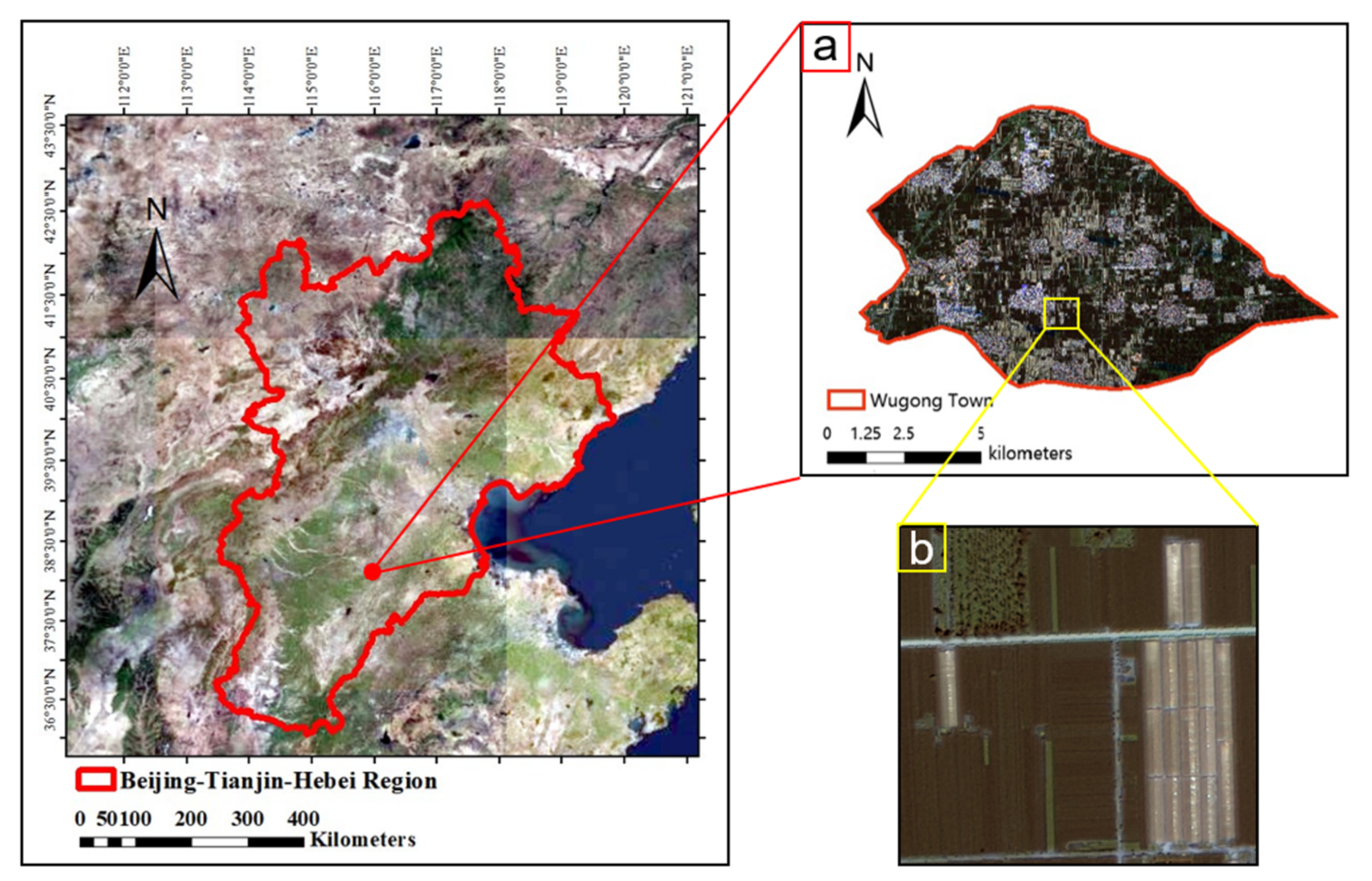
Figure 1. Overview of the study area. (a) the study area Wugong Town. (b) the fragment of the study area with greenhouses.
Remotesensing 14 05064 g001
Figure 2. False color image of the study area.
Remotesensing 14 05064 g002
Figure 3. Algorithm flow chart.
Remotesensing 14 05064 g003
Figure 4. Implementation flow of YOLOX inserting CBAM and ASFF modules. Reg represents the loss function of location; Obj represents the loss function of determining part for positive samples; Cls represents the loss function of classification.
Remotesensing 14 05064 g004
Figure 5. The specific process of weighted feature fusion of ASFF module.
Remotesensing 14 05064 g005
Figure 6. DeepLabv3+ Model Network Structure.
Remotesensing 14 05064 g006
Figure 7. Greenhouse quantity extraction results for concentrated distribution (the first line) and scattered distribution (the second line). (a): Ground Truth (b): YOLOX (c): YOLOX+CBAM (d): YOLOX+ASFF (e): YOLOX+CBAM+ASFF.
Remotesensing 14 05064 g007
Figure 8. Loss function change curve. (a): Training dataset; (b): Verification dataset.
Remotesensing 14 05064 g008
Figure 9. Greenhouse segmentation results of deeplabV3+ models with different backbone networks (a): MobileNet_4_200 (b): ResNet_4_200 (c): Xception (d): MobileNet_8_200 (e): ResNet_8_200 (f): manually labeled.
Remotesensing 14 05064 g009
Figure 10. Greenhouse segmentation results of different network structures (a): Ground Truth (b): UNet (c): ENVINET5 (d): DeeplabV3+.
Remotesensing 14 05064 g010
Figure 11. Extraction results of greenhouse for concentrated distribution (the first line) and scattered distribution (the second line). (a): input (b): object-based result (c): pixel-based result (d): final result.
Remotesensing 14 05064 g011
Table 1. Spectral information of GF-2 camera.
Imaging EquipmentGround Resolution/mBandsSpectral Range/μm
Panchromatic camera0.81Panchromatic band0.45~0.90
Multispectral camera3.24Band 1: Blue0.45~0.52
Band 2: Green0.52~0.59
Band 3: Red0.63~0.69
Band 4: Near-infrared0.77~0.89
Table 2. Detection results of different YOLO improvement methods (IoU threshold is 0.65).
The Network TypeRecall/%Precision/%F1-Score/%mAP/%
YOLOV596.5794.8696.0095.06
YOLOX97.7196.1496.9296.65
YOLOX+CBAM98.6196.2597.4297.62
YOLOX+ASFF98.1296.1597.1396.98
YOLOX+CBAM+ASFF (proposed)98.6196.4097.5097.65
Table 3. Comparative testing of DeeplabV3+ models of five groups of backbone neural networks.
Number of Neural Network GroupsBackboneBatch-SizeEpochTraining Time/hValidation Set mIoUValidation Set Acc
Group1:MobileNet_4_200MobileNetV242003.270.9560.992
Group2:MobileNet_8_200MobileNetV282002.980.9560.992
Group3:ResNet_4_200ResNet-10142006.550.9570.992
Group4:ResNet_8_200ResNet-10182005.780.9580.992
Group5:Xception_4_200Aligned Xception42007.980.9430.990
Table 4. Comparative test of different network structures in greenhouse area extraction.
Network TypeAccuracy/%mIoU/%
ENVINet594.288.5
UNet98.793.3
DeeplabV3+99.295.8
Publisher’s Note: MDPI stays neutral with regard to jurisdictional claims in published maps and institutional affiliations.