


Experimental Study of Accuracy of High-Rate GNSS in Context of Structural Health Monitoring


Abstract
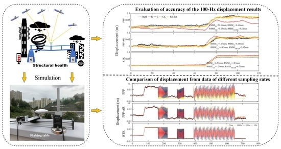
1. Introduction
2. Methods and Materials
2.1. Real-Time Kinematic Positioning
2.2. Precise Point Positioning
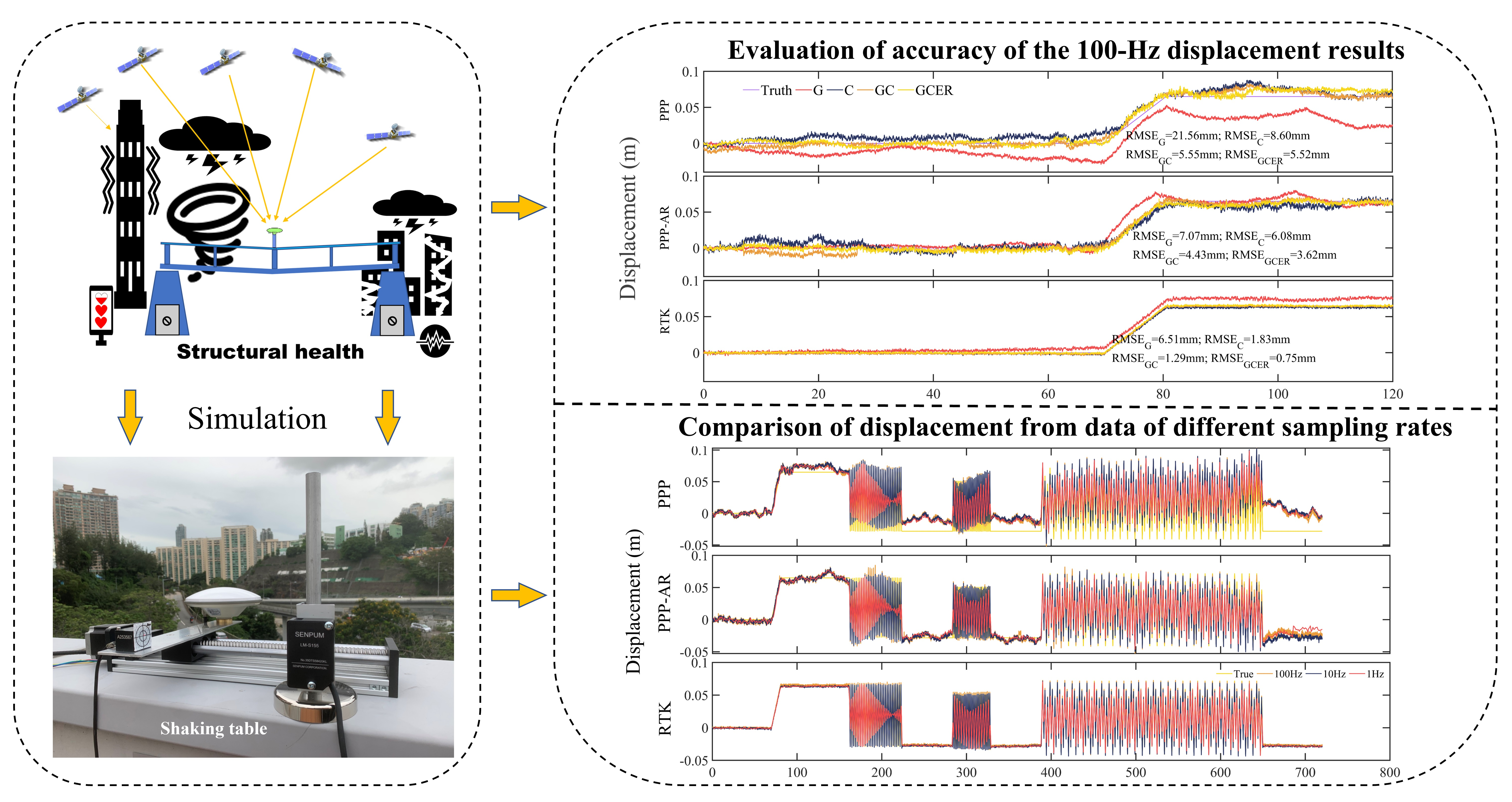
2.3. Experiments
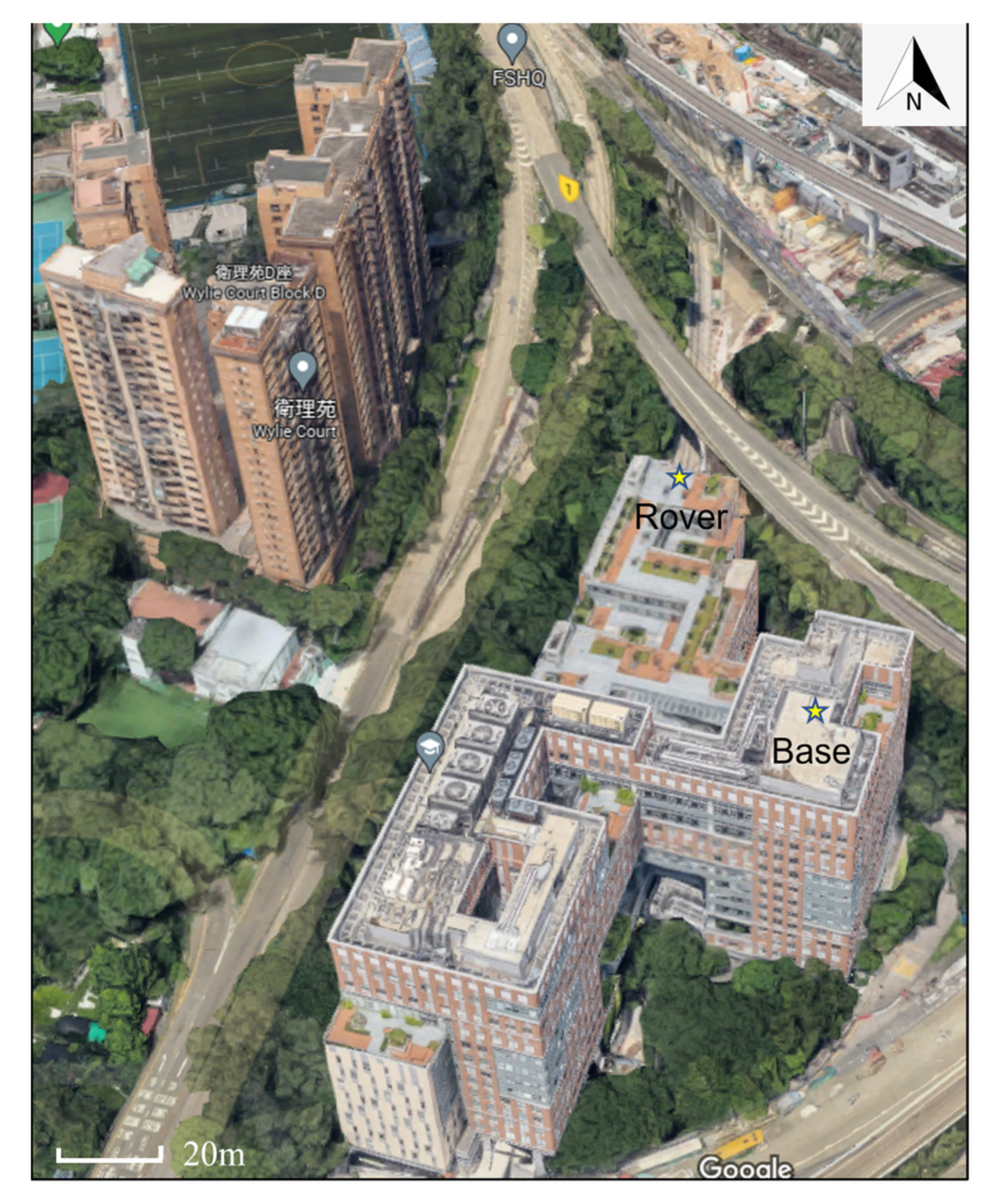
2.3.1. Set Up of Shaking Table
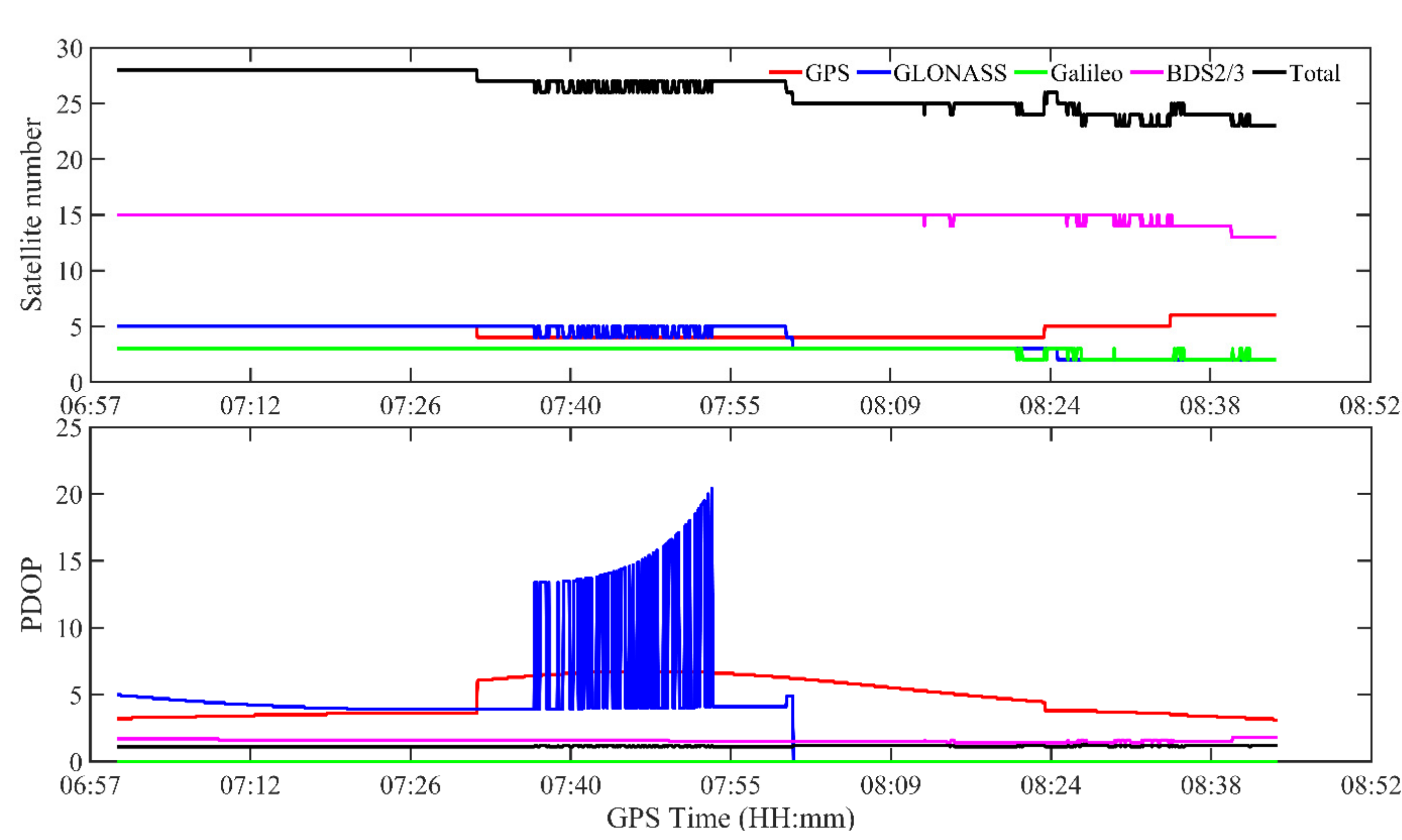
2.3.2. Data Collection and Processing
3. Results and Discussion
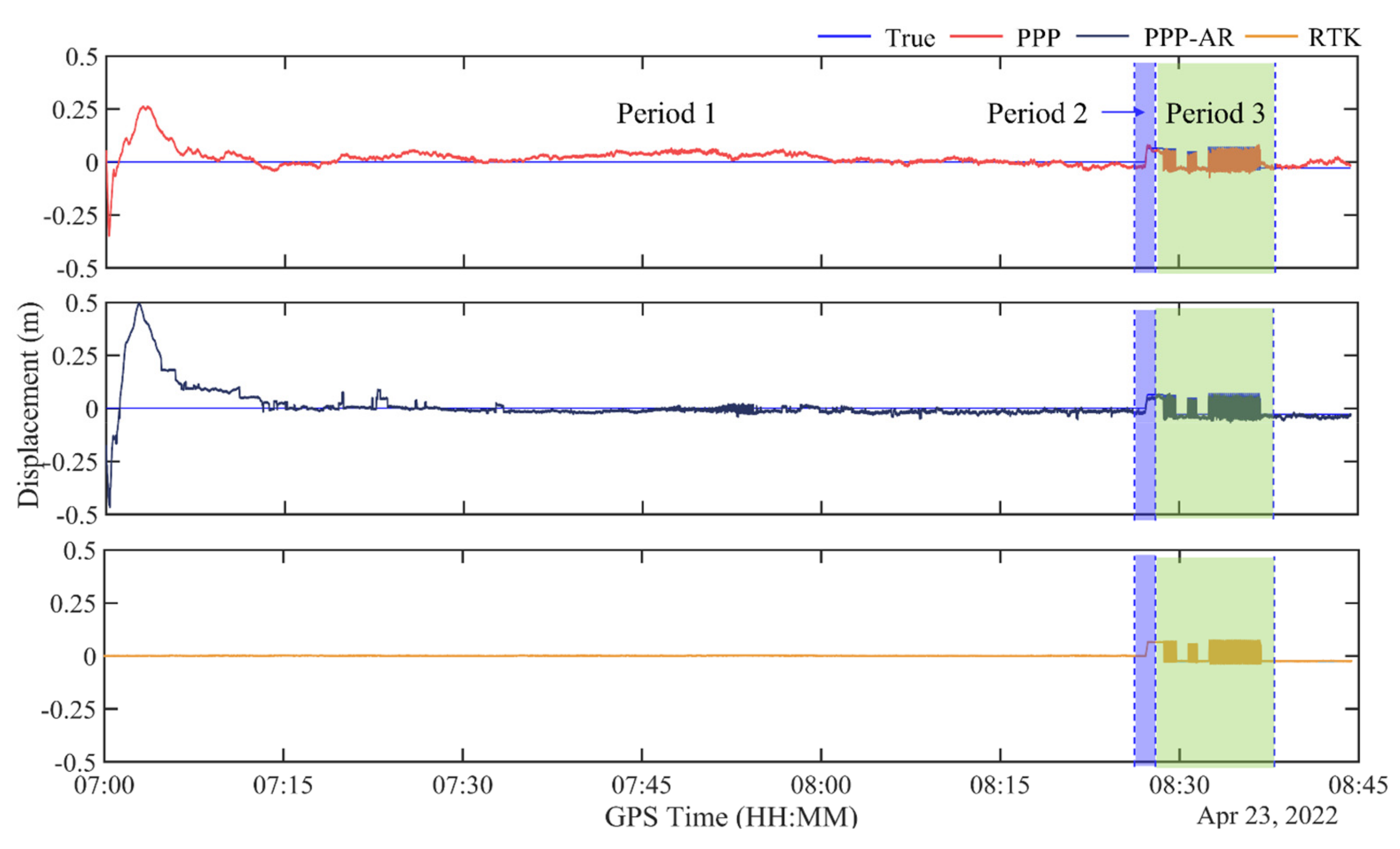
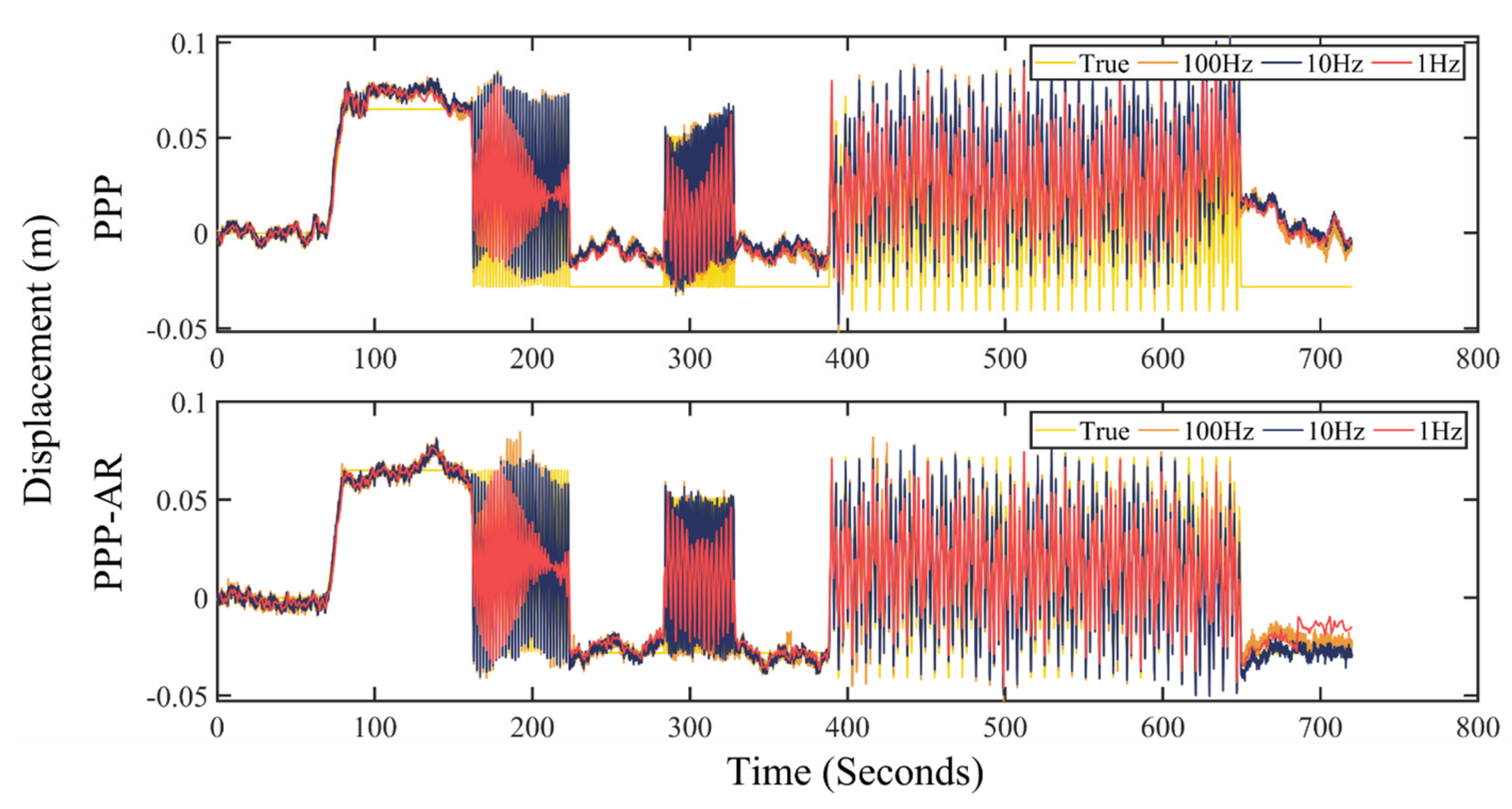
3.1. Displacement Time Series
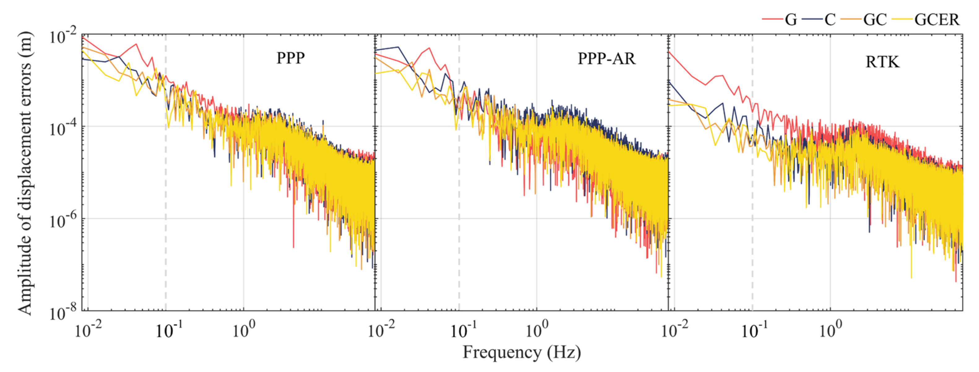
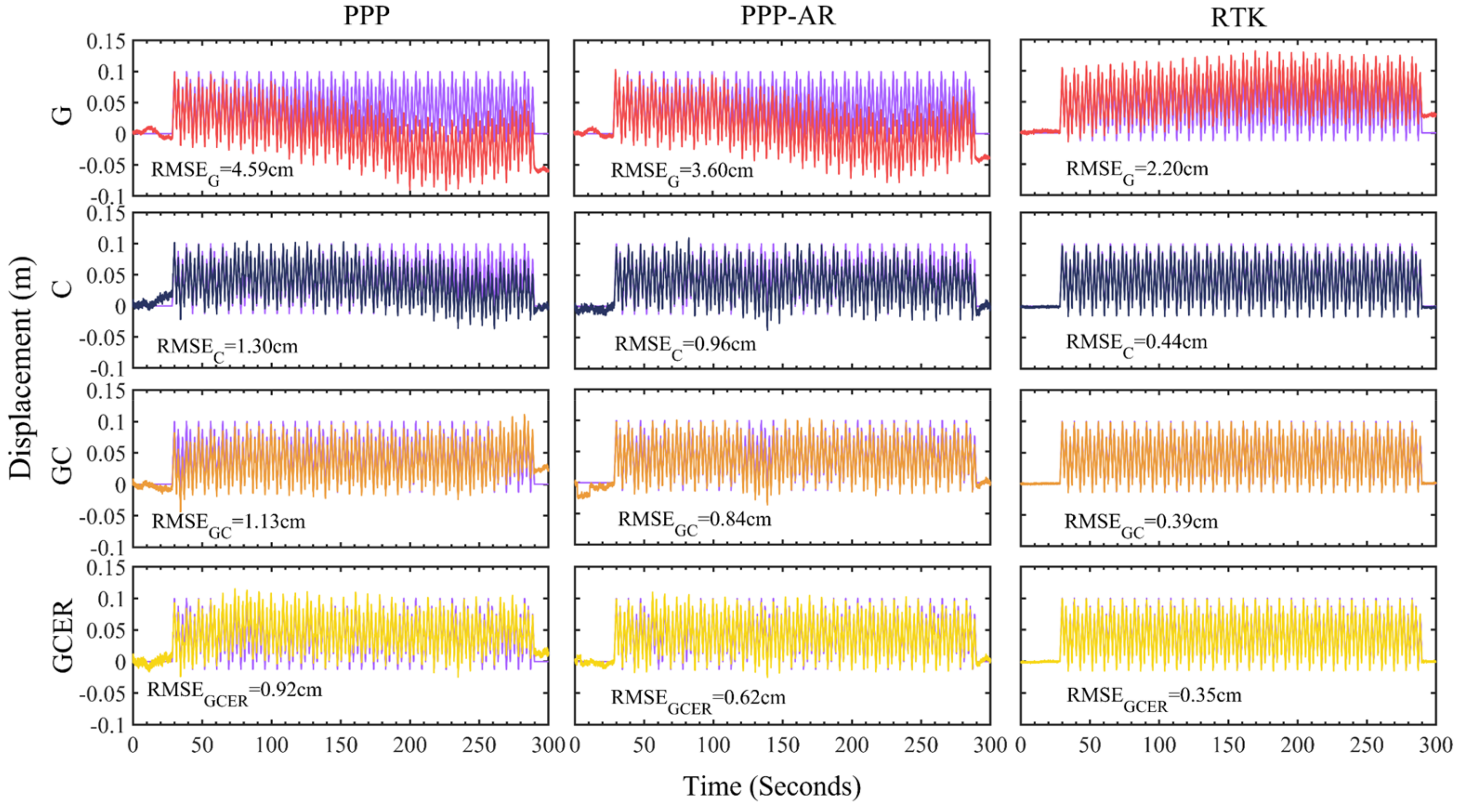
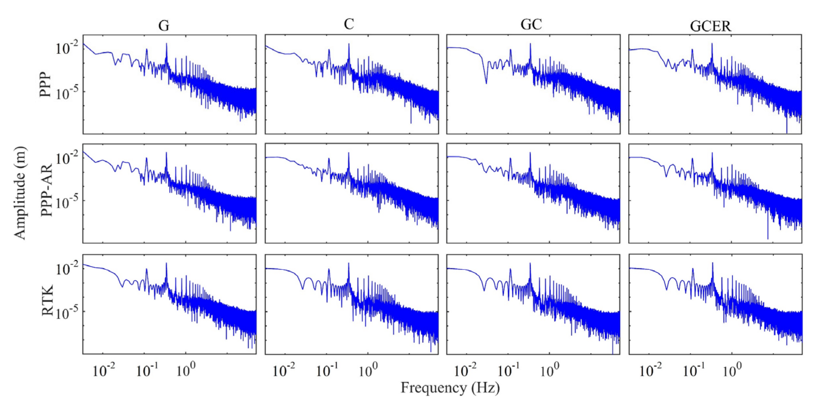
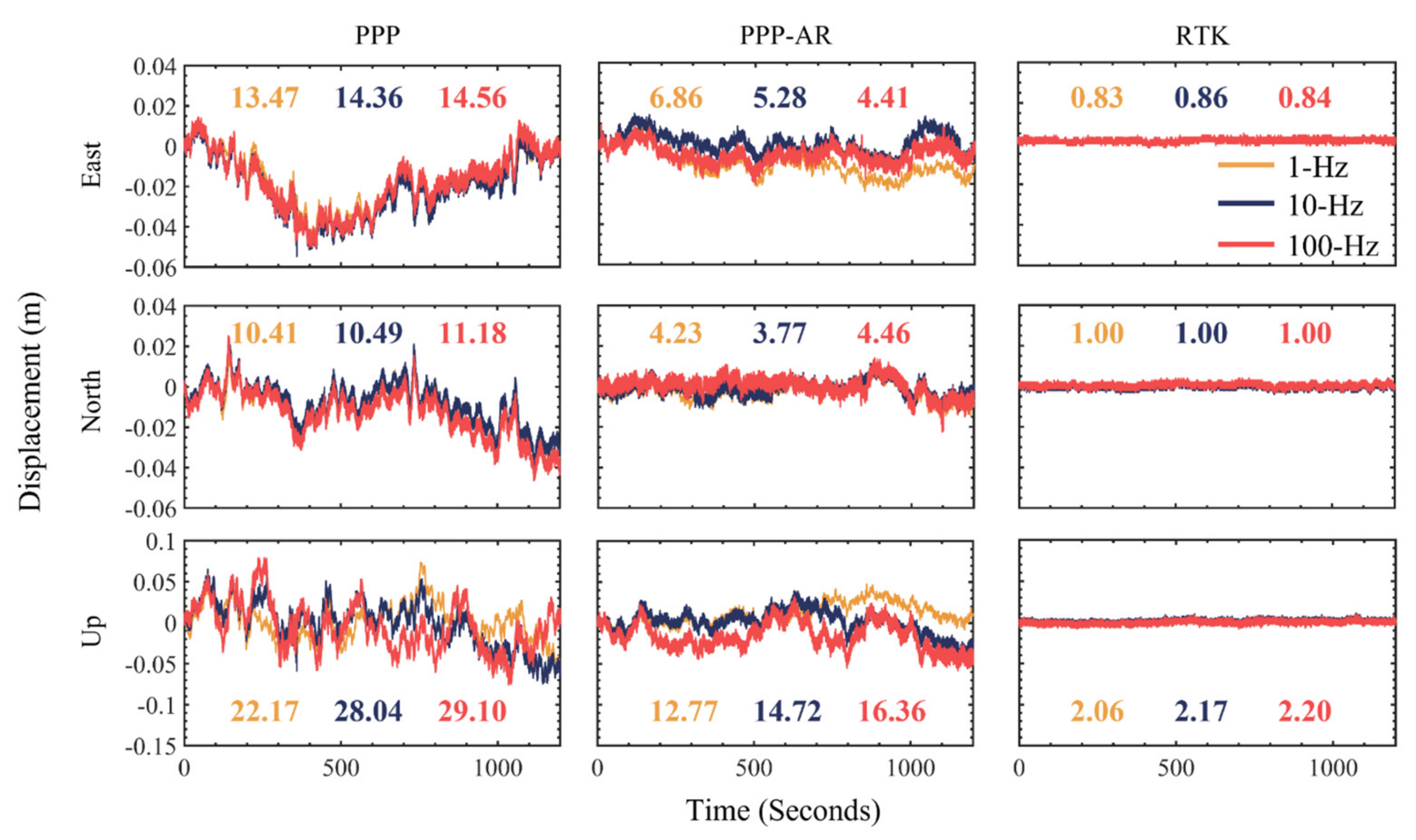
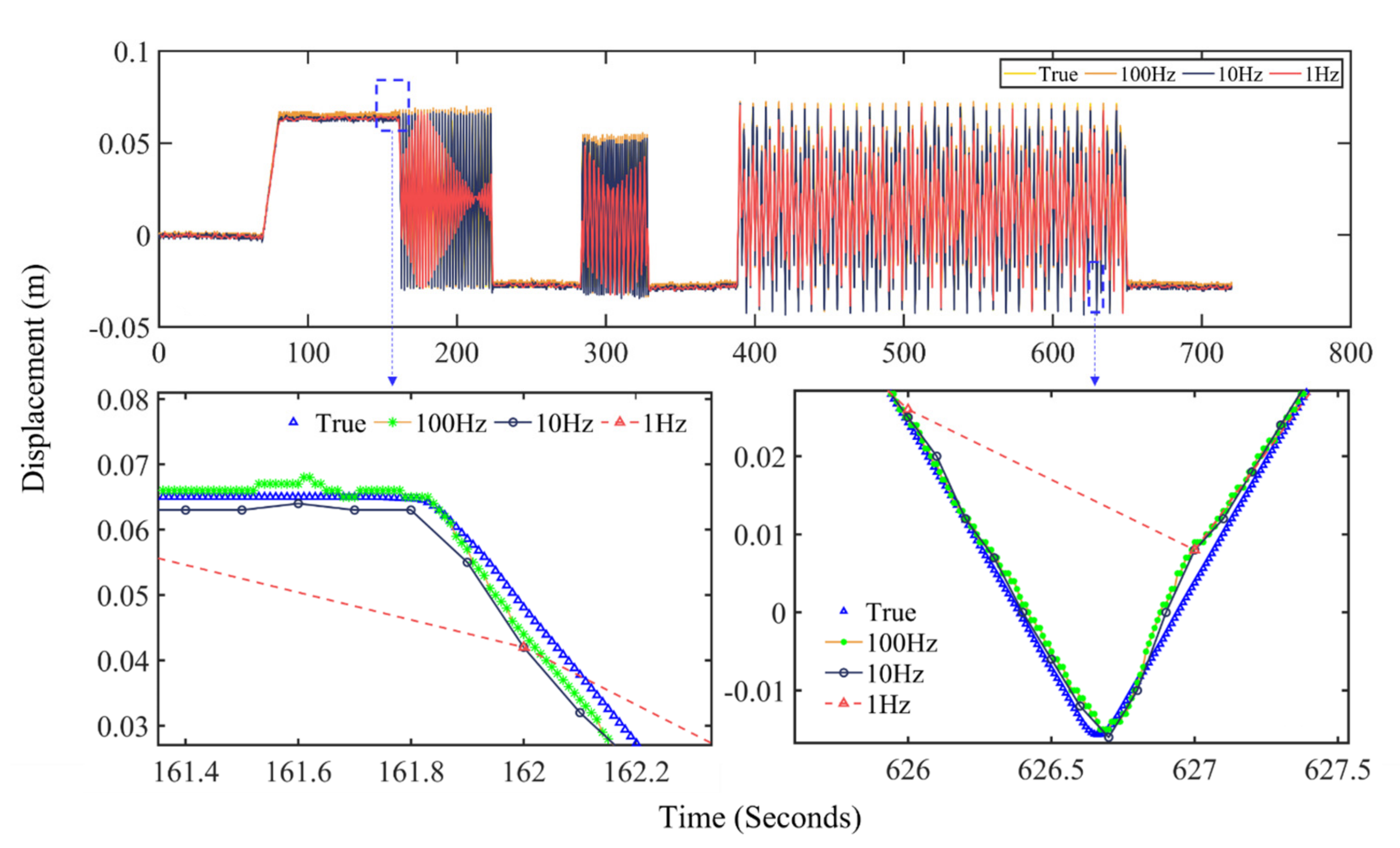
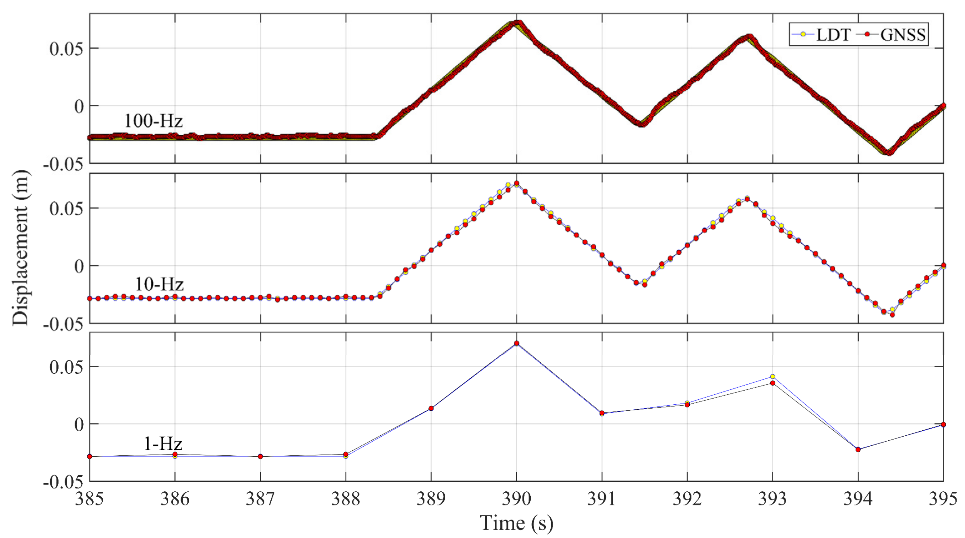
3.2. Evaluation of Accuracy of the 100-Hz Displacement Time Series
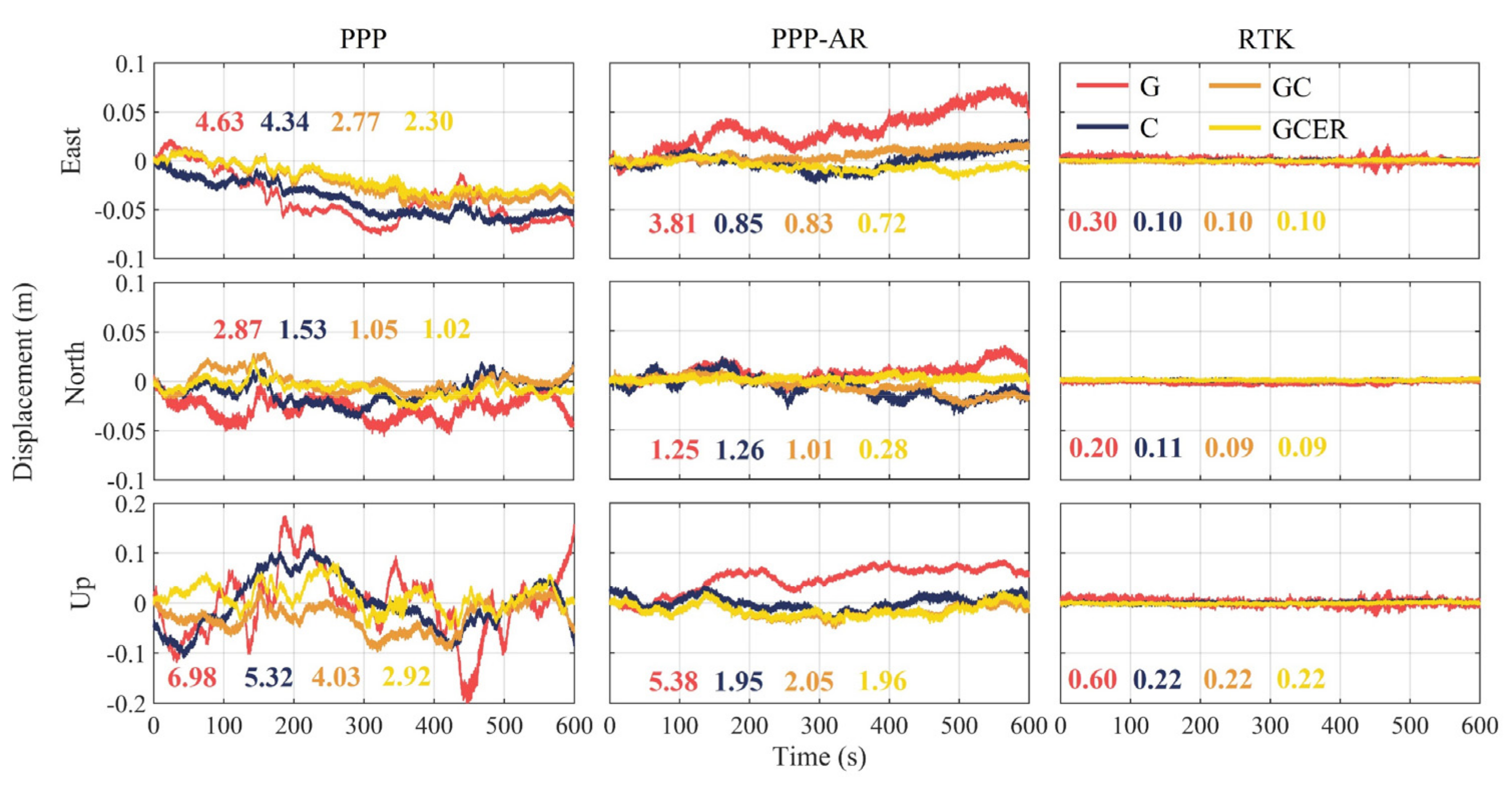
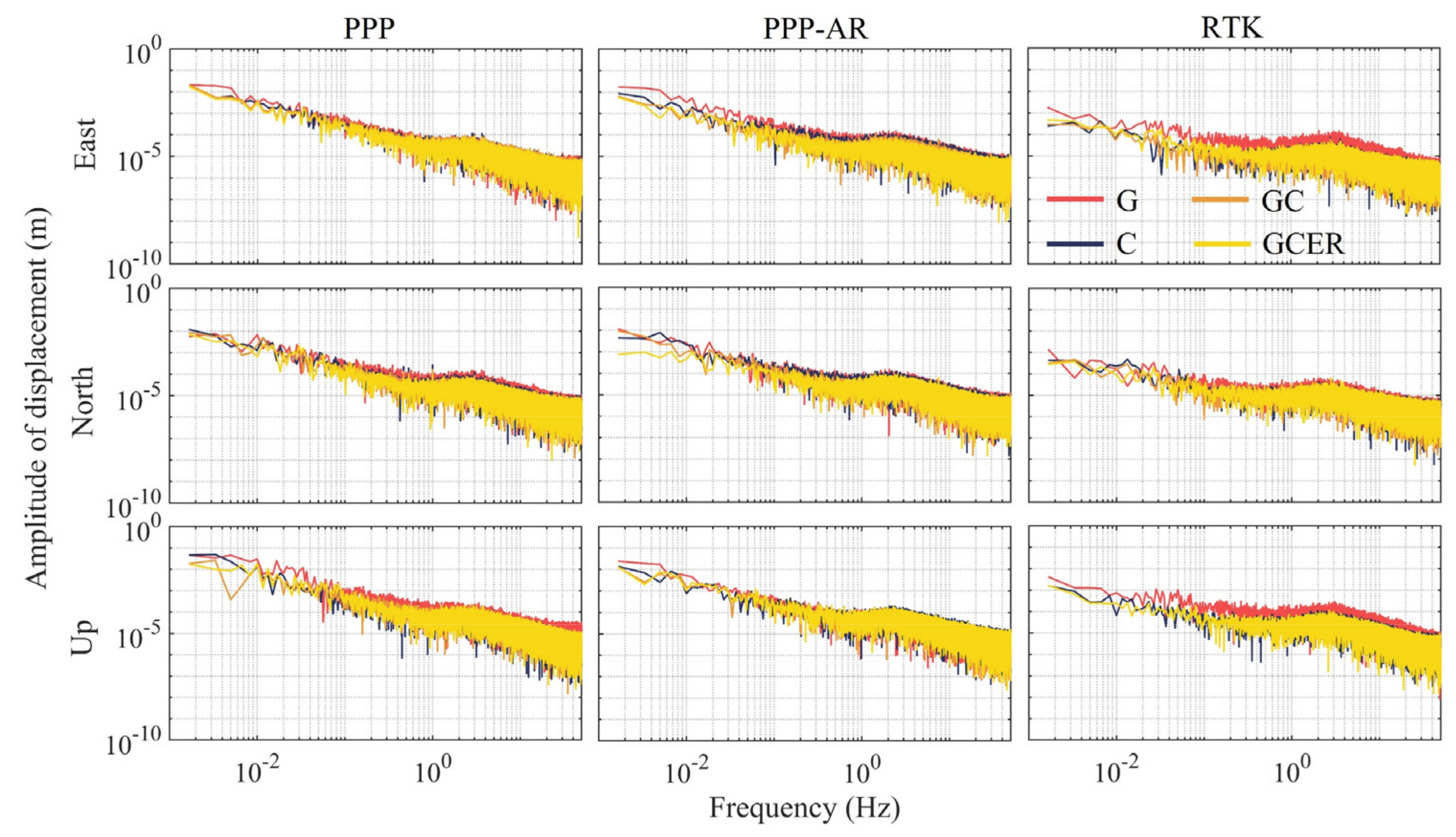
3.2.1. Stationary Test
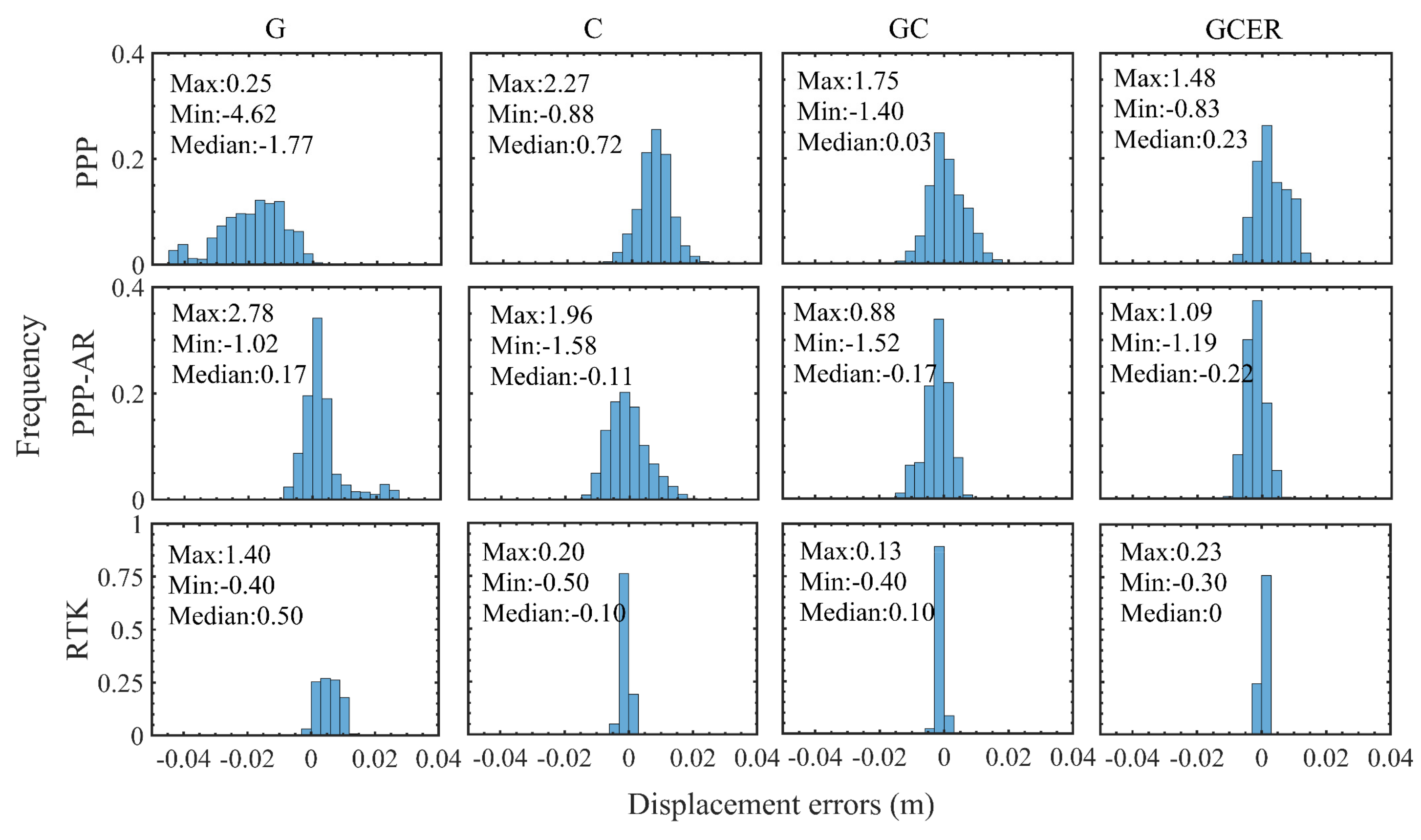
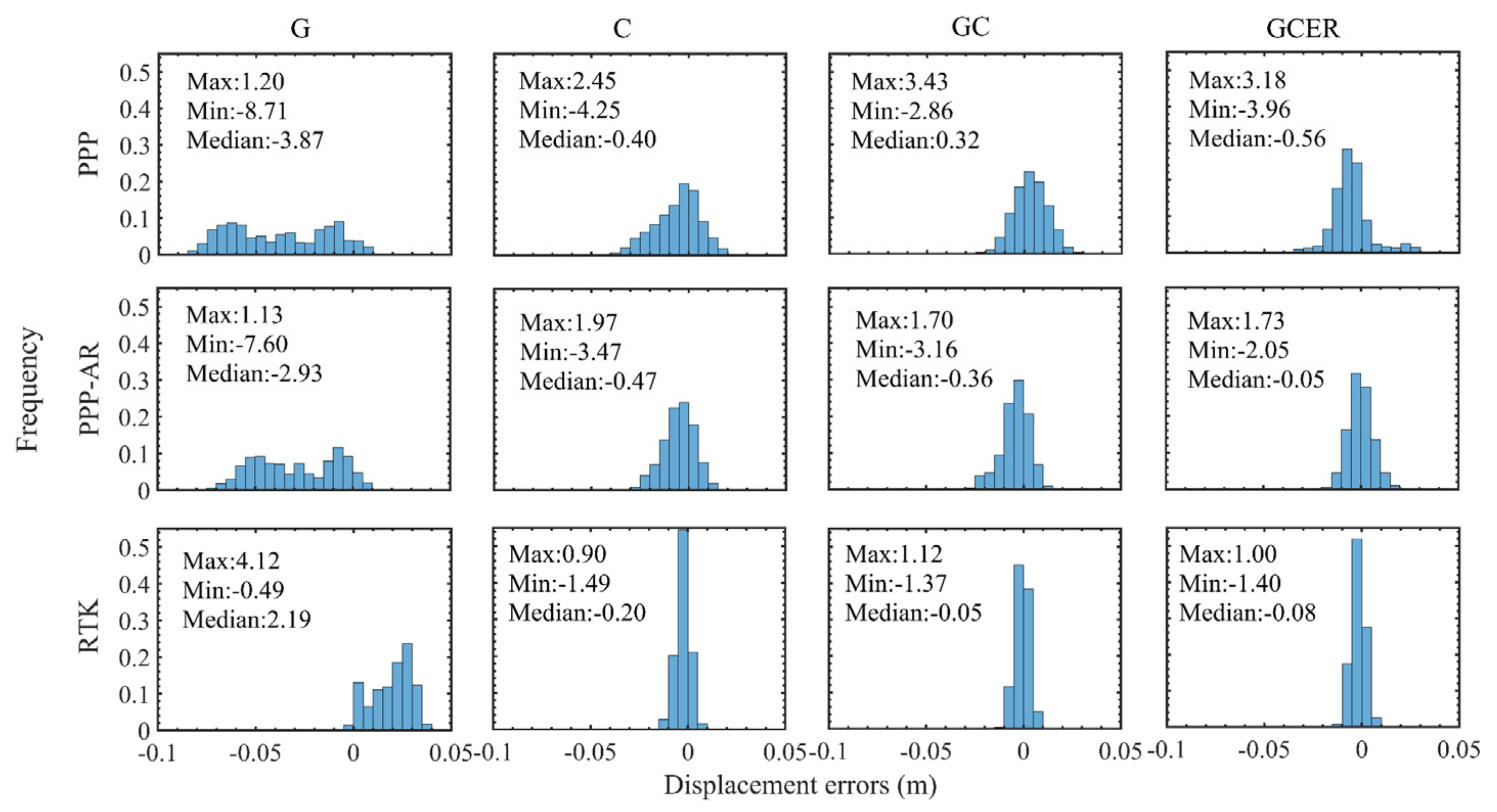
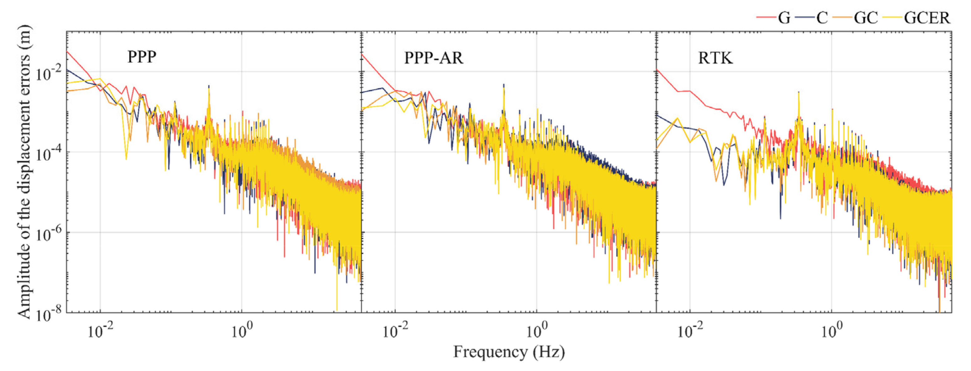
3.2.2. Quasi-Static Motion Test
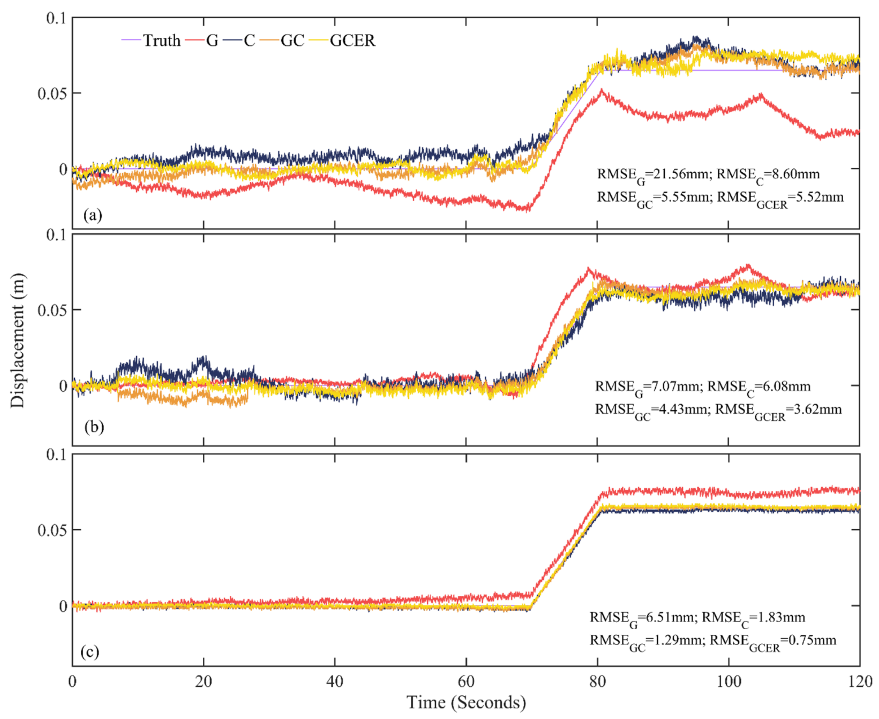
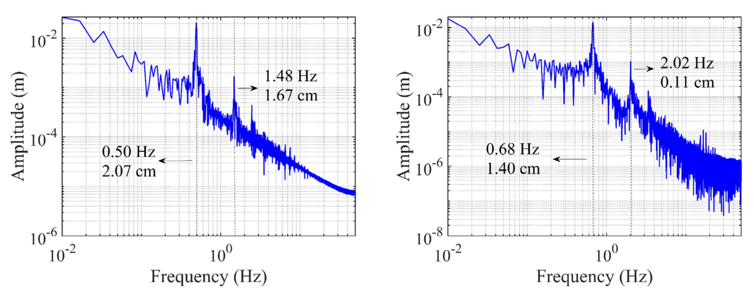
3.2.3. Sinusoidal Motion Test
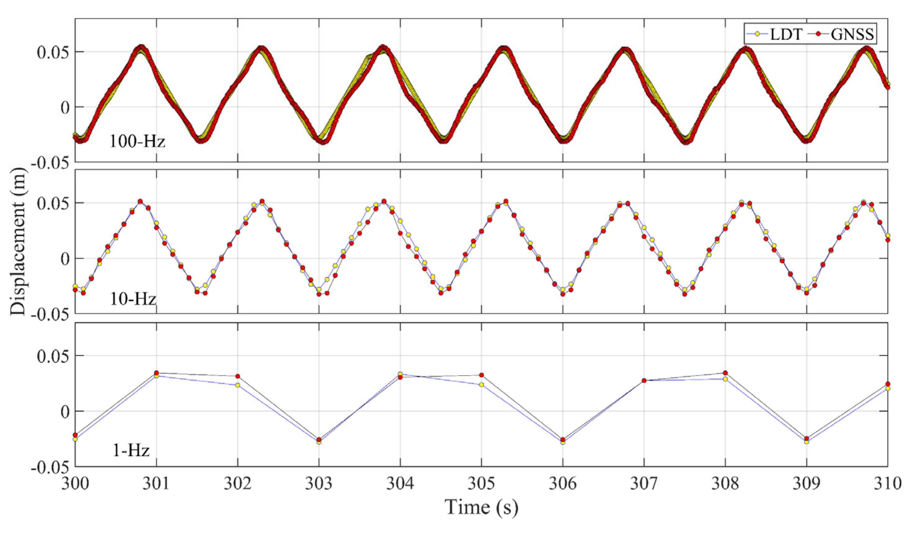
3.3. Comparison of Displacement Results from Data of Different Sampling Rates
4. Conclusions
Author Contributions
Funding
Data Availability Statement
Acknowledgments
Conflicts of Interest
Appendix A


References
- Chan, W.S.; Xu, Y.L.; Ding, X.L.; Xiong, Y.L.; Dai, W.J. Assessment of dynamic measurement accuracy of GPS in three directions. J. Surv. Eng. 2006, 132, 108–117. [Google Scholar] [CrossRef]
- Górski, P. Dynamic characteristic of tall industrial chimney estimated from GPS measurement and frequency domain decomposition. Eng. Struct. 2017, 148, 277–292. [Google Scholar] [CrossRef]
- Xie, L.; Xu, W.; Ding, X. Precursory motion and deformation mechanism of the 2018 Xe Pian-Xe Namnoy dam Collapse, Laos: Insights from satellite radar interferometry. Int. J. Appl. Earth Obs. Geoinf. 2022, 109. [Google Scholar] [CrossRef]
- Meng, X.; Wang, J.; Han, H. Optimal GPS/accelerometer integration algorithm for monitoring the vertical structural dynamics. J. Appl. Geod. 2014, 8, 265–272. [Google Scholar] [CrossRef]
- Geng, J.; Pan, Y.; Li, X.; Guo, J.; Liu, J.; Chen, X.; Zhang, Y. Noise characteristics of high-rate multi-GNSS for subdaily crustal deformation monitoring. J. Geophys. Res. Solid Earth 2018, 123, 1987–2002. [Google Scholar] [CrossRef]
- Zumberge, J.F.; Heflin, M.B.; Jefferson, D.C.; Watkins, M.M.; Webb, F.H. Precise point positioning for the efficient and robust analysis of GPS data from large networks. J. Geophys. Res. Solid Earth 1997, 102, 5005–5017. [Google Scholar] [CrossRef]
- Zhong, P.; Ding, X.; Yuan, L.; Xu, Y.; Kwok, K.; Chen, Y. Sidereal filtering based on single differences for mitigating GPS multipath effects on short baselines. J. Geod. 2010, 84, 145–158. [Google Scholar] [CrossRef]
- Chen, Q.; Jiang, W.; Meng, X.; Jiang, P.; Wang, K.; Xie, Y.; Ye, J. Vertical deformation monitoring of the suspension bridge tower using GNSS: A case study of the forth road bridge in the UK. Remote Sens. 2018, 10, 364. [Google Scholar] [CrossRef]
- Dai, W.; Huang, D.; Cai, C. Multipath mitigation via component analysis methods for GPS dynamic deformation monitoring. GPS Solut. 2014, 18, 417–428. [Google Scholar] [CrossRef]
- Xi, R.; Jiang, W.; Meng, X.; Chen, H.; Chen, Q. Bridge monitoring using BDS-RTK and GPS-RTK techniques. Measurement 2018, 120, 128–139. [Google Scholar] [CrossRef]
- Xi, R.; Zhou, X.; Jiang, W.; Chen, Q. Simultaneous estimation of dam displacements and reservoir level variation from GPS measurements. Measurement 2018, 122, 247–256. [Google Scholar] [CrossRef]
- Xu, P.; Shi, C.; Fang, R.; Liu, J.; Niu, X.; Zhang, Q.; Yanagidani, T. High-rate precise point positioning (PPP) to measure seismic wave motions: An experimental comparison of GPS PPP with inertial measurement units. J. Geod. 2013, 87, 361–372. [Google Scholar] [CrossRef]
- Tang, X.; Liu, Z.; Roberts, G.W.; Hancock, C.M. PPP-derived tropospheric ZWD augmentation from local CORS network tested on bridge monitoring points. Adv. Space Res. 2022, 69, 3633–3643. [Google Scholar] [CrossRef]
- Tu, R.; Wang, R.; Ge, M.; Walter, T.R.; Ramatschi, M.; Milkereit, C.; Dahm, T. Cost-effective monitoring of ground motion related to earthquakes, landslides, or volcanic activity by joint use of a single-frequency GPS and a MEMS accelerometer. Geophys. Res. Lett. 2013, 40, 3825–3829. [Google Scholar] [CrossRef]
- Yigit, C.O.; El-Mowafy, A.; Anil Dindar, A.; Bezcioglu, M.; Tiryakioglu, I. Investigating Performance of high-rate GNSS-PPP and PPP-AR for structural health monitoring: Dynamic tests on shake table. J. Surv. Eng. 2021, 147, 05020011. [Google Scholar] [CrossRef]
- Li, X.; Ge, M.; Zhang, X.; Zhang, Y.; Guo, B.; Wang, R.; Wickert, J. Real-time high-rate co-seismic displacement from ambiguity-fixed precise point positioning: Application to earthquake early warning. Geophys. Res. Lett. 2013, 40, 295–300. [Google Scholar] [CrossRef]
- Yigit, C.O.; Gurlek, E. Experimental testing of high-rate GNSS precise point positioning (PPP) method for detecting dynamic vertical displacement response of engineering structures. Geomat. Nat. Hazards Risk 2017, 8, 893–904. [Google Scholar] [CrossRef]
- Yu, W.; Peng, H.; Pan, L.; Dai, W.; Qu, X.; Ren, Z. Performance assessment of high-rate GPS/BDS precise point positioning for vibration monitoring based on shaking table tests. Adv. Space Res. 2022, 69, 2362–2375. [Google Scholar] [CrossRef]
- Yu, J.; Meng, X.; Shao, X.; Yan, B.; Yang, L. Identification of dynamic displacements and modal frequencies of a medium-span suspension bridge using multimode GNSS processing. Eng. Struct. 2014, 81, 432–443. [Google Scholar] [CrossRef]
- Moschas, F.; Avallone, A.; Saltogianni, V.; Stiros, S.C. Strong motion displacement waveforms using 10-Hz precise point positioning GPS: An assessment based on free oscillation experiments. Earthq. Eng. Struct. Dyn. 2014, 43, 1853–1866. [Google Scholar] [CrossRef]
- Msaewe, H.A.; Psimoulis, P.A.; Hancock, C.M.; Roberts, G.W.; Bonenberg, L. Monitoring the response of Severn Suspension Bridge in the United Kingdom using multi-GNSS measurements. Struct. Control. Health Monit. 2021, 28, e2830. [Google Scholar] [CrossRef]
- Cantieni, R. Transportation Research Board, National Research Council, Washington, DC, USA. In Dynamic Load Testing of Highway Bridges; National Research Council: Washington, DC, USA, 1984. [Google Scholar]
- Kaloop, M.R.; Hu, J.W.; Elbeltagi, E. Adjustment and assessment of the measurements of low and high sampling frequencies of GPS real-time monitoring of structural movement. ISPRS Int. J. Geo-Inf. 2016, 5, 222. [Google Scholar] [CrossRef]
- Yi, T.H.; Li, H.N.; Gu, M. Experimental assessment of high-rate GPS receivers for deformation monitoring of bridge. Measurement 2013, 46, 420–432. [Google Scholar] [CrossRef]
- Moschas, F.; Stiros, S. Measurement of the dynamic displacements and of the modal frequencies of a short-span pedestrian bridge using GPS and an accelerometer. Eng. Struct. 2011, 33, 10–17. [Google Scholar] [CrossRef]
- Moschas, F.; Stiros, S. PLL bandwidth and noise in 100 Hz GPS measurements. GPS Solut. 2015, 19, 173–185. [Google Scholar] [CrossRef]
- Paziewski, J.; Sieradzki, R.; Baryla, R. Detection of structural vibration with high-rate precise point positioning: Case study results based on 100 Hz multi-GNSS observables and shake-table simulation. Sensors 2019, 19, 4832. [Google Scholar] [CrossRef]
- Häberling, S.; Rothacher, M.; Zhang, Y.; Clinton, J.F.; Geiger, A. Assessment of high-rate GPS using a single-axis shake table. J. Geod. 2015, 89, 697–709. [Google Scholar] [CrossRef]
- Shu, Y.; Fang, R.; Li, M.; Shi, C.; Li, M.; Liu, J. Very high-rate GPS for measuring dynamic seismic displacements without aliasing: Performance evaluation of the variometric approach. GPS Solut. 2018, 22, 121. [Google Scholar] [CrossRef]
- Yang, Y.; Mao, Y.; Sun, B. Basic performance and future developments of BeiDou global navigation satellite system. Satell. Navig. 2020, 1, 1–8. [Google Scholar] [CrossRef]
- Odolinski, R.; Teunissen, P.J. Best integer equivariant estimation: Performance analysis using real data collected by low-cost, single-and dual-frequency, multi-GNSS receivers for short-to long-baseline RTK positioning. J. Geod. 2020, 94, 1–17. [Google Scholar] [CrossRef]
- Ge, M.; Gendt, G.; Rothacher, M.A.; Shi, C.; Liu, J. Resolution of GPS carrier-phase ambiguities in precise point positioning (PPP) with daily observations. J. Geod. 2008, 82, 389–399. [Google Scholar] [CrossRef]
- Teunissen, P. The Least-Squares Ambiguity Decorrelation Adjustment: A Method for Fast GPS Ambiguity Estimation. J. Geod. 1999, 73, 587–593. [Google Scholar] [CrossRef]
- Chan, W.S.; Xu, Y.L.; Ding, X.L.; Dai, W.J. An integrated GPS–accelerometer data processing technique for structural deformation monitoring. J. Geod. 2006, 80, 705–719. [Google Scholar] [CrossRef]
- Zhang, Y.; Chen, J.; Gong, X.; Chen, Q. The update of BDS-2 TGD and its impact on positioning. Adv. Space Res. 2020, 65, 2645–2661. [Google Scholar] [CrossRef]
- Montenbruck, O.; Steigenberger, P.; Prange, L.; Deng, Z.; Zhao, Q.; Perosanz, F.; Schaer, S. The Multi-GNSS Experiment (MGEX) of the International GNSS Service (IGS)–achievements, prospects and challenges. Adv. Space Res. 2017, 59, 1671–1697. [Google Scholar] [CrossRef]
- Geng, J.; Chen, X.; Pan, Y.; Zhao, Q. A modified phase clock/bias model to improve PPP ambiguity resolution at Wuhan University. J. Geod. 2019, 93, 2053–2067. [Google Scholar] [CrossRef]
- Böhm, J.; Möller, G.; Schindelegger, M.; Pain, G.; Weber, R. Development of an improved empirical model for slant delays in the troposphere (GPT2w). GPS Solut. 2015, 19, 433–441. [Google Scholar] [CrossRef]
- Psimoulis, P.; Pytharouli, S.; Karambalis, D.; Stiros, S. Potential of Global Positioning System (GPS) to measure frequencies of oscillations of engineering structures. J. Sound Vib. 2008, 318, 606–623. [Google Scholar] [CrossRef]
- Jiang, Y.; Gao, Y.; Zhou, P.; Gao, Y.; Huang, G. Real-time cascading PPP-WAR based on Kalman filter considering time-correlation. J. Geod. 2021, 95, 1–15. [Google Scholar] [CrossRef]
- Psimoulis, P.A.; Houlié, N.; Behr, Y. Real-time magnitude characterization of large earthquakes using the predominant period derived from 1 Hz GPS data. Geophys. Res. Lett. 2018, 45, 517–526. [Google Scholar] [CrossRef]
- Michel, C.; Kelevitz, K.; Houlié, N.; Edwards, B.; Psimoulis, P.; Su, Z.; Giardini, D. The potential of high-rate GPS for strong ground motion assessment. Bull. Seismol. Soc. Am. 2017, 107, 1849–1859. [Google Scholar] [CrossRef]


| Parameters | PPP | PPP-AR | RTK |
|---|---|---|---|
| Frequency | Dual | Dual | Dual |
| Sampling rate | 0.01s (100 Hz) | 0.01s (100 Hz) | 0.01s (100 Hz) |
| Elevation mask | 10º | 10º | 10º |
| Tropospheric model | Zenith: GPT2w Mapping function: VMF1 [38] | Zenith: GPT2w Mapping function: VMF1 [38] | |
| Ionospheric model | IF | IF | |
| Orbit | Final products from GFZ (5 min) | Rapid products from WUM (1 min) | Broadcast ephemerides |
| Clock | Final products from GFZ (30 s) | Rapid products from WUM (30 s) | Broadcast ephemerids |
| Estimator | Kalman filter | Kalman filter | Kalman filter |
| GNSS System | 1st Peak (Ref: 0.11/1.04) | 2nd Peak (Ref: 0.34/2.68) | ||||
|---|---|---|---|---|---|---|
| PPP | PPP-AR | RTK | PPP | PPP-AR | RTK | |
| G | 0.11/0.97 | 0.11/0.98 | 0.11/1.07 | 0.34/2.63 | 0.34/2.64 | 0.34/2.65 |
| C | 0.11/1.02 | 0.11/1.03 | 0.11/1.03 | 0.34/2.64 | 0.34/2.66 | 0.34/2.67 |
| GC | 0.11/0.99 | 0.11/0.99 | 0.11/1.05 | 0.34/2.66 | 0.34/2.69 | 0.34/2.67 |
| GCER | 0.11/1.00 | 0.11/1.02 | 0.11/1.04 | 0.34/2.69 | 0.34/2.68 | 0.34/2.68 |
| Sampling Rate | PPP | PPP-AR | RTK |
|---|---|---|---|
| 1-Hz | 16.34 | 6.06 | 4.66 |
| 10-Hz | 17.18 (5.1%) | 6.58 (8.6%) | 4.79 (2.8%) |
| 100-Hz | 17.96 (9.9%) | 7.01 (15.6%) | 4.91 (5.4%) |
Publisher’s Note: MDPI stays neutral with regard to jurisdictional claims in published maps and institutional affiliations. |
© 2022 by the authors. Licensee MDPI, Basel, Switzerland. This article is an open access article distributed under the terms and conditions of the Creative Commons Attribution (CC BY) license (https://creativecommons.org/licenses/by/4.0/).
Share and Cite
Qu, X.; Shu, B.; Ding, X.; Lu, Y.; Li, G.; Wang, L. Experimental Study of Accuracy of High-Rate GNSS in Context of Structural Health Monitoring. Remote Sens. 2022, 14, 4989. https://doi.org/10.3390/rs14194989
Qu X, Shu B, Ding X, Lu Y, Li G, Wang L. Experimental Study of Accuracy of High-Rate GNSS in Context of Structural Health Monitoring. Remote Sensing. 2022; 14(19):4989. https://doi.org/10.3390/rs14194989
Chicago/Turabian StyleQu, Xuanyu, Bao Shu, Xiaoli Ding, Yangwei Lu, Guopeng Li, and Li Wang. 2022. "Experimental Study of Accuracy of High-Rate GNSS in Context of Structural Health Monitoring" Remote Sensing 14, no. 19: 4989. https://doi.org/10.3390/rs14194989
APA StyleQu, X., Shu, B., Ding, X., Lu, Y., Li, G., & Wang, L. (2022). Experimental Study of Accuracy of High-Rate GNSS in Context of Structural Health Monitoring. Remote Sensing, 14(19), 4989. https://doi.org/10.3390/rs14194989