


An Observation Density Based Method for Independent Baseline Searching in GNSS Network Solution

Abstract

1. Introduction
2. Data and Method
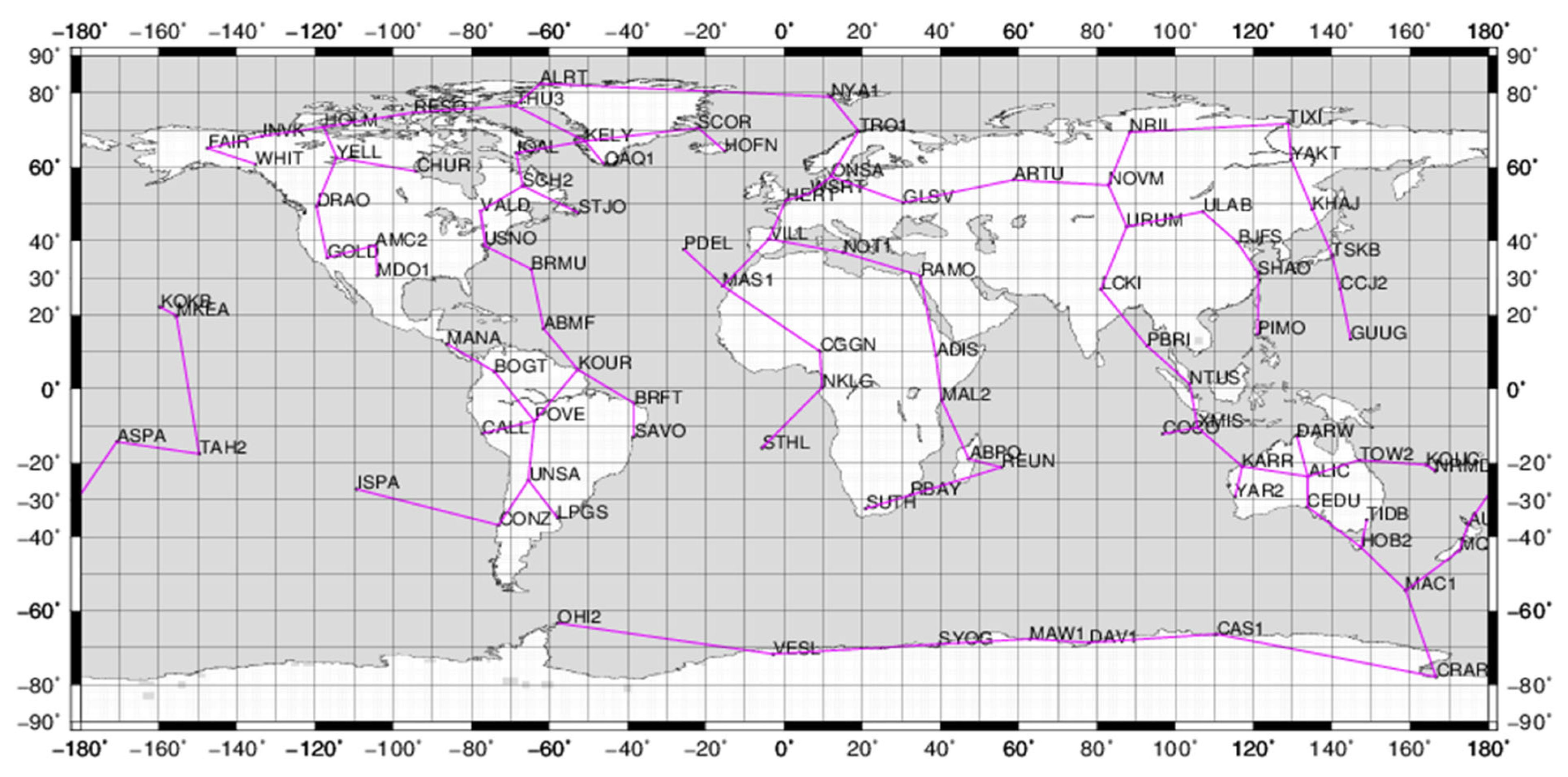
2.1. Data
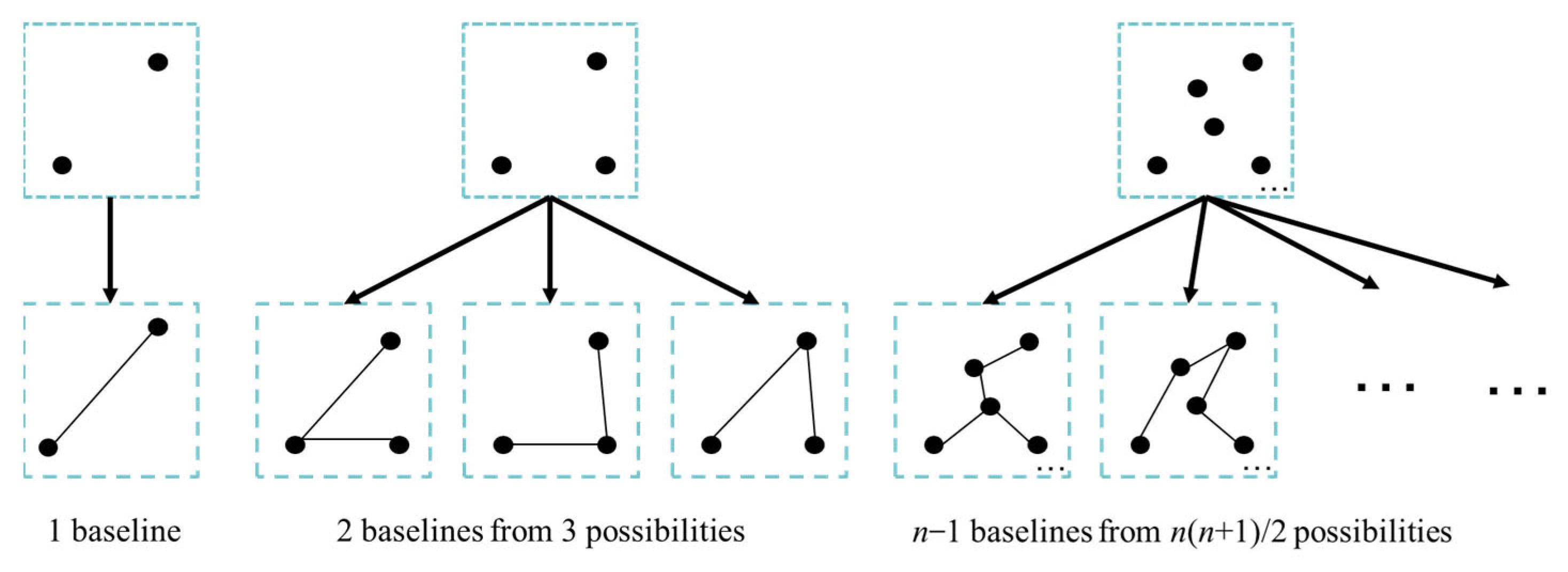
2.2. MST
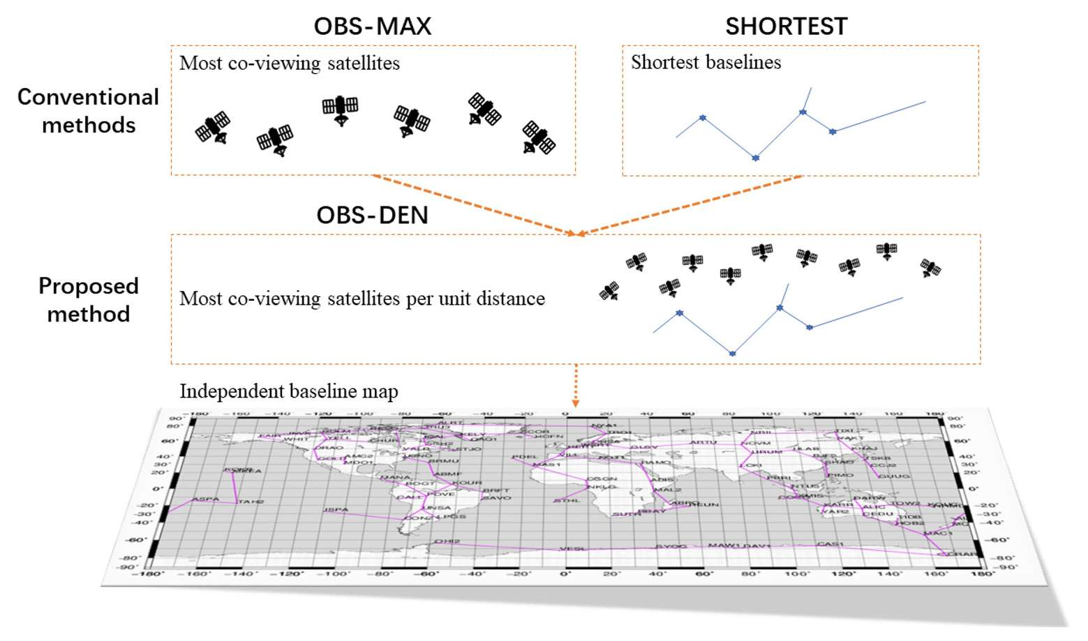
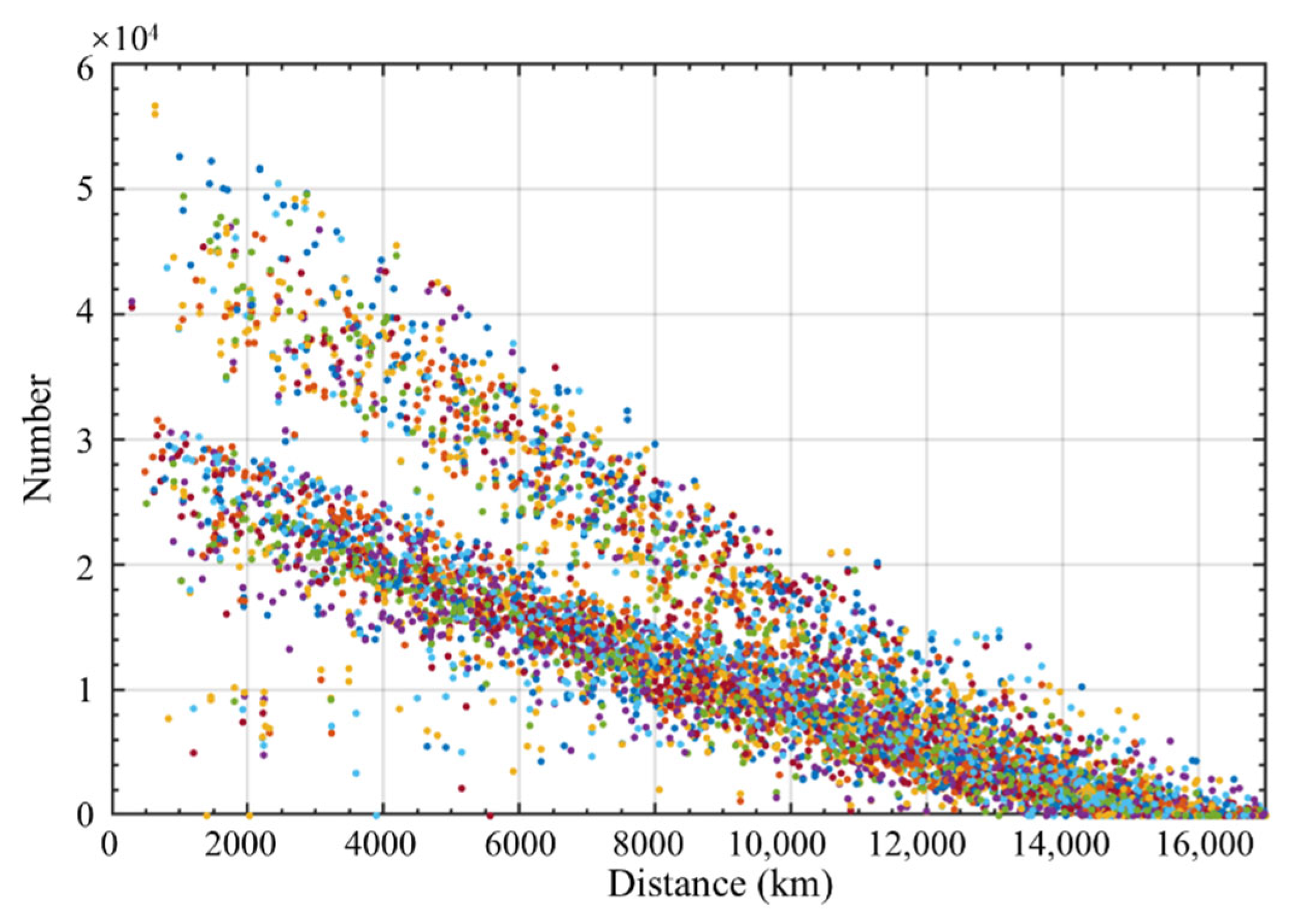
2.3. The Criteria—Distance, Observation, and Others
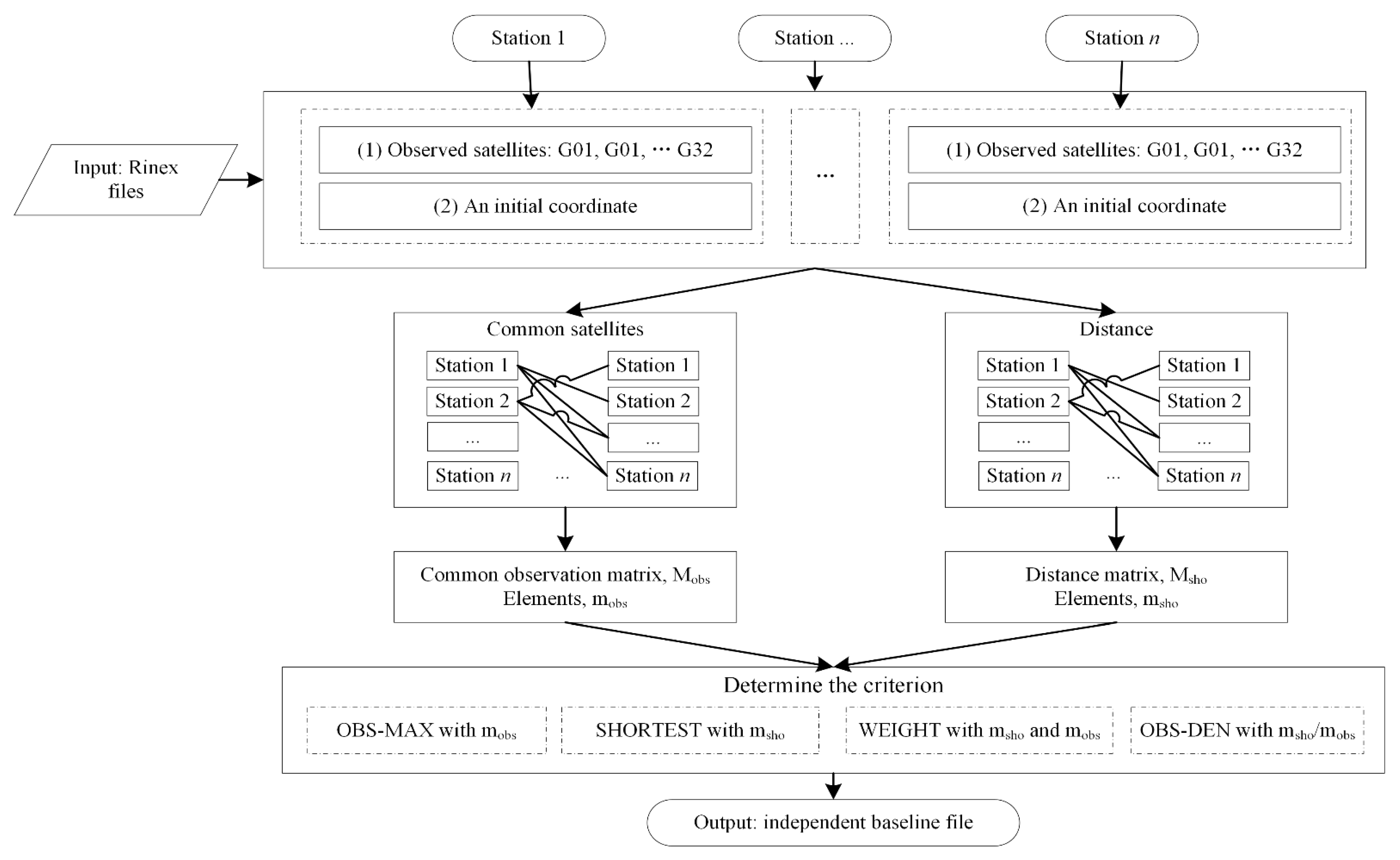
2.4. The Calculation Process of the Independent Baseline
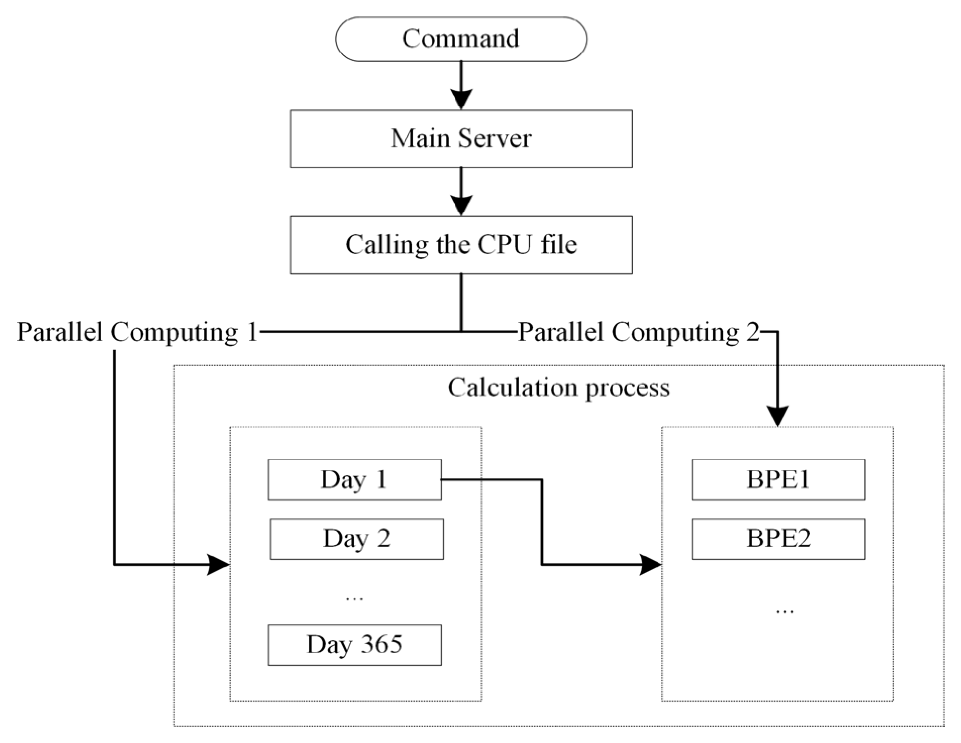
2.5. Parallel Computation
3. Results
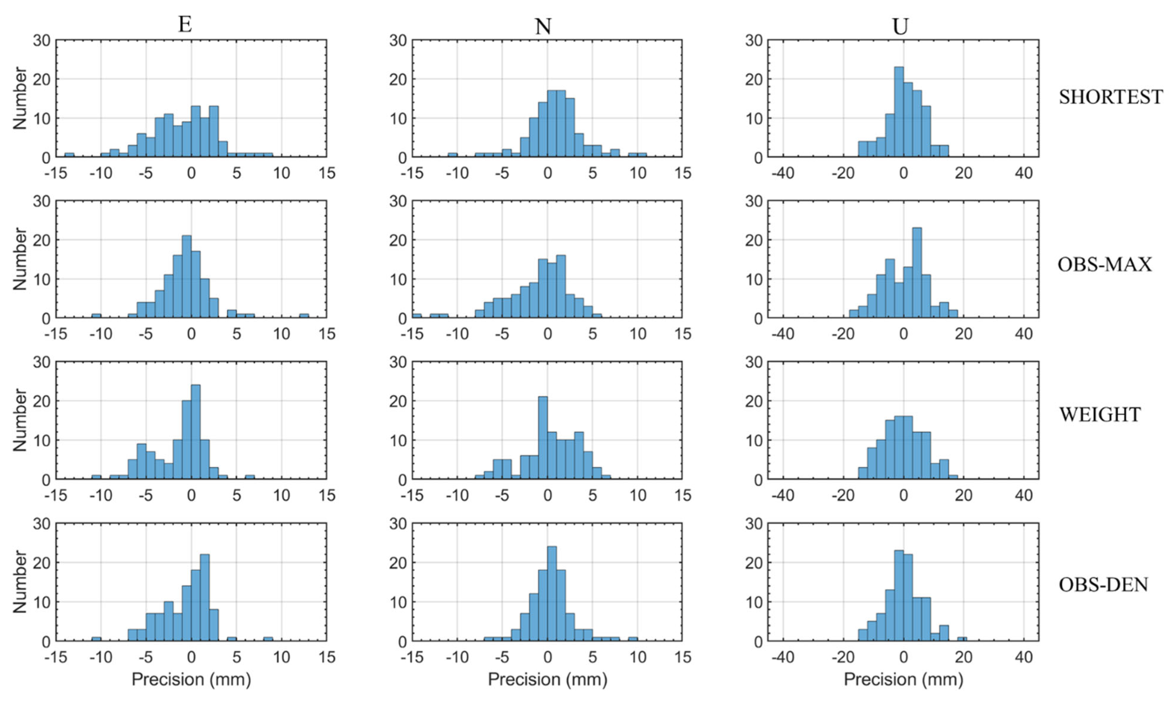
3.1. Single-Day Solution
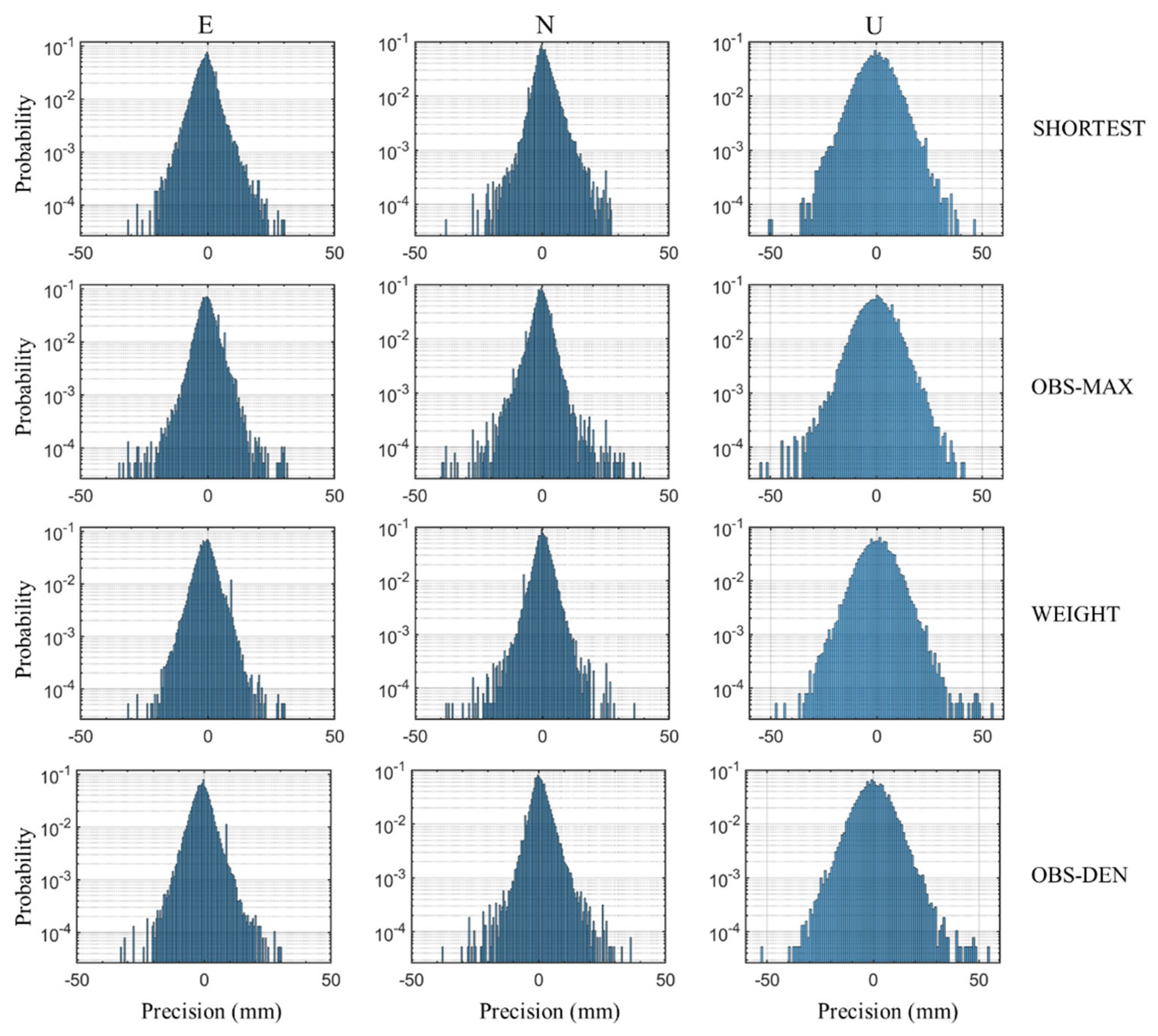
3.2. One-Year Statistical Results
4. Discussion
5. Conclusions
Author Contributions
Funding
Data Availability Statement
Acknowledgments
Conflicts of Interest
References
- Rodriguez-Solano, C.; Hugentobler, U.; Steigenberger, P.; Bloßfeld, M.; Fritsche, M. Reducing the draconitic errors in GNSS geodetic products. J. Geod. 2014, 88, 559–574. [Google Scholar] [CrossRef]
- Stępniak, K.; Bock, O.; Bosser, P.; Wielgosz, P. Outliers and uncertainties in GNSS ZTD estimates from double-difference processing and precise point positioning. GPS Solut. 2022, 26, 74. [Google Scholar] [CrossRef]
- Sun, M.; Liu, L.; Yan, W.; Liu, J.; Liu, T.; Xu, G. Performance analysis of BDS B1C/B2a PPP using different models and MGEX products. Surv. Rev. 2022, 1–12. [Google Scholar] [CrossRef]
- Yang, Y.; Mao, Y.; Sun, B. Basic performance and future developments of BeiDou global navigation satellite system. Satell. Navig. 2020, 1, 1. [Google Scholar] [CrossRef]
- Zajdel, R.; Sośnica, K.; Dach, R.; Bury, G.; Prange, L.; Jäggi, A. Network effects and handling of the geocenter motion in multi-GNSS processing. J. Geophys. Res. Solid Earth 2019, 124, 5970–5989. [Google Scholar] [CrossRef]
- Specht, C.; Specht, M.; Dąbrowski, P. Comparative analysis of active geodetic networks in Poland. Int. Multidiscip. Sci. GeoConf. SGEM 2017, 17, 163–176. [Google Scholar]
- Xu, G.; Xu, Y. GPS: Theory, Algorithms and Applications; Springer: Berlin, Germany, 2016. [Google Scholar]
- Dach, R.; Walser, P. Bernese GNSS Software, Version 5.2; University of Bern: Bern, Switzerland, 2015.
- Herring, T.; King, R.; McClusky, S. Introduction to Gamit/Globk; Massachusetts Institute of Technology: Cambridge, MA, USA, 2010. [Google Scholar]
- Gilad, E.-T. Graph theory applications to GPS networks. GPS Solut. 2001, 5, 31–38. [Google Scholar]
- Graham, R.L.; Hell, P. On the history of the minimum spanning tree problem. Ann. Hist. Comput. 1985, 7, 43–57. [Google Scholar] [CrossRef]
- Cui, Y.; Chen, Z.; Li, L.; Zhang, Q.; Lu, Z. An efficient parallel computing strategy for the processing of large GNSS network datasets. GPS Solut. 2021, 25, 36. [Google Scholar] [CrossRef]
- Stepniak, K.; Bock, O.; Wielgosz, P. Reduction of ZTD outliers through improved GNSS data processing and screening strategies. Atmos. Meas. Tech. 2018, 11, 1347–1361. [Google Scholar] [CrossRef]
- Liu, T.; Xu, T.; Nie, W.; Li, M.; Fang, Z.; Du, Y.; Jiang, Y.; Xu, G. Optimal Independent Baseline Searching for Global GNSS Networks. J. Surv. Eng. 2021, 147, 5020010. [Google Scholar] [CrossRef]
- Krypiak-Gregorczyk, A. Ionosphere response to three extreme events occurring near spring equinox in 2012, 2013 and 2015, observed by regional GNSS-TEC model. J. Geod. 2019, 93, 931–951. [Google Scholar] [CrossRef]
- Chen, Z.; Zhiping, L.; Yang, C.; Hao, L. Parallel computing of GNSS data based on Bernese processing engine. J. Geod. Geodyn. 2013, 33, 79–82. [Google Scholar]
- Li, L.; Lu, Z.; Chen, Z.; Cui, Y.; Sun, D.; Wang, Y.; Kuang, Y.; Wang, F. GNSSer: Objected-oriented and design pattern-based software for GNSS data parallel processing. J. Spat. Sci. 2019, 66, 27–47. [Google Scholar] [CrossRef]
- Jiang, C.; Xu, T.; Du, Y.; Sun, Z.; Xu, G. A parallel equivalence algorithm based on MPI for GNSS data processing. J. Spat. Sci. 2019, 66, 513–532. [Google Scholar] [CrossRef]
- Naidoo, K. MiSTree: A Python package for constructing and analysing Minimum Spanning Trees. arXiv 2019, arXiv:1910.08562. [Google Scholar] [CrossRef]
- Kruskal, J.B. On the shortest spanning subtree of a graph and the traveling salesman problem. Proc. Am. Math. Soc. 1956, 7, 48–50. [Google Scholar] [CrossRef]
- Spira, P.M.; Pan, A. On finding and updating spanning trees and shortest paths. SIAM J. Comput. 1975, 4, 375–380. [Google Scholar] [CrossRef]
- Prim, R.C. Shortest connection networks and some generalizations. Bell Syst. Tech. J. 1957, 36, 1389–1401. [Google Scholar] [CrossRef]
- Cui, Y.; Lv, Z.; Li, L.; Chen, Z.; Sun, D.; Kwong, Y. A Fast Parallel Processing Strategy of Double Difference Model for GNSS Huge Networks. Acta Geod. Cartogr. Sin. 2017, 46, 48–56. [Google Scholar]
- Paziewski, J.; Kurpinski, G.; Wielgosz, P.; Stolecki, L.; Sieradzki, R.; Seta, M.; Oszczak, S.; Castillo, M.; Martin-Porqueras, F. Towards Galileo+ GPS seismology: Validation of high-rate GNSS-based system for seismic events characterisation. Measurement 2020, 166, 108236. [Google Scholar] [CrossRef]
- Fotiou, A.; Pikridas, C.; Rossikopoulos, D.; Chatzinikos, M. The effect of independent and trivial GPS baselines on the adjustment of networks in everyday engineering practice. In Proceedings of the International Symposium on Modern Technologies, Education and Professional Practice in Geodesy and Related Fields, Sofia, Bulgaria, 5–6 November 2009; pp. 201–212. [Google Scholar]
- Geng, J.; Mao, S. Massive GNSS network analysis without baselines: Undifferenced ambiguity resolution. J. Geophys. Res. Solid Earth 2021, 126, e2020JB021558. [Google Scholar] [CrossRef]
- Hua, C. Application Research of Method of Large GNSS Network Realtime Data Rapid Solution. Ph.D. Thesis, Wuhan University, Wuhan, China, 2010. [Google Scholar]
- Liu, T.; Yu, Z.; Ding, Z.; Nie, W.; Xu, G. Observation of Ionospheric Gravity Waves Introduced by Thunderstorms in Low Latitudes China by GNSS. Remote Sens. 2021, 13, 4131. [Google Scholar] [CrossRef]
- Dao, T.; Harima, K.; Carter, B.; Currie, J.; McClusky, S.; Brown, R.; Rubinov, E.; Choy, S. Regional Ionospheric Corrections for High Accuracy GNSS Positioning. Remote Sens. 2022, 14, 2463. [Google Scholar] [CrossRef]
- Bakuła, M.; Przestrzelski, P.; Kaźmierczak, R. Reliable technology of centimeter GPS/GLONASS surveying in forest environments. IEEE Trans. Geosci. Remote Sens. 2014, 53, 1029–1038. [Google Scholar] [CrossRef]
- Wang, P.; Liu, H.; Yang, Z.; Shu, B.; Xu, X.; Nie, G. Evaluation of Network RTK Positioning Performance Based on BDS-3 New Signal System. Remote Sens. 2021, 14, 2. [Google Scholar] [CrossRef]
- Liu, J.; Zhang, B.; Liu, T.; Xu, G.; Ji, Y.; Sun, M.; Nie, W.; He, Y. An Efficient UD Factorization Implementation of Kalman Filter for RTK Based on Equivalent Principle. Remote Sens. 2022, 14, 967. [Google Scholar] [CrossRef]
- Siejka, Z. Validation of the accuracy and convergence time of real time kinematic results using a single galileo navigation system. Sensors 2018, 18, 2412. [Google Scholar] [CrossRef]


| MEAN (mm) | STD (mm) | RMS (mm) | ||||||||
|---|---|---|---|---|---|---|---|---|---|---|
| E | N | U | E | N | U | E | N | U | 3D | |
| SHORTEST | −0.99 | 0.89 | −0.53 | 3.66 | 3.15 | 5.97 | 3.79 | 3.28 | 6.00 | 7.81 |
| OBS-MAX | −0.70 | −1.09 | 0.13 | 2.83 | 3.53 | 7.28 | 2.92 | 3.69 | 7.28 | 8.67 |
| WEIGHT | −1.45 | 0.29 | 0.00 | 2.96 | 3.07 | 6.95 | 3.30 | 3.08 | 6.95 | 8.29 |
| OBS-DEN | −0.70 | 0.38 | 0.19 | 2.78 | 2.41 | 6.25 | 2.86 | 2.44 | 6.25 | 7.30 |
| RMS | Probability | ||||||
|---|---|---|---|---|---|---|---|
| E (mm) | N (mm) | U (mm) | 3D | <ε | <2ε | <3ε | |
| SHORTEST | 4.38 | 4.21 | 7.63 | 9.75 | 71.89% | 96.17% | 99.38% |
| OBS-MAX | 3.92 | 3.94 | 7.79 | 9.57 | 71.96% | 96.54% | 99.16% |
| WEIGHT | 4.14 | 3.92 | 7.78 | 9.64 | 71.82% | 96.77% | 99.41% |
| OBS-DEN | 4.31 | 4.15 | 7.68 | 9.73 | 72.49% | 96.45% | 99.33% |
Publisher’s Note: MDPI stays neutral with regard to jurisdictional claims in published maps and institutional affiliations. |
© 2022 by the authors. Licensee MDPI, Basel, Switzerland. This article is an open access article distributed under the terms and conditions of the Creative Commons Attribution (CC BY) license (https://creativecommons.org/licenses/by/4.0/).
Share and Cite
Liu, T.; Du, Y.; Nie, W.; Liu, J.; Ma, Y.; Xu, G. An Observation Density Based Method for Independent Baseline Searching in GNSS Network Solution. Remote Sens. 2022, 14, 4717. https://doi.org/10.3390/rs14194717
Liu T, Du Y, Nie W, Liu J, Ma Y, Xu G. An Observation Density Based Method for Independent Baseline Searching in GNSS Network Solution. Remote Sensing. 2022; 14(19):4717. https://doi.org/10.3390/rs14194717
Chicago/Turabian StyleLiu, Tong, Yujun Du, Wenfeng Nie, Jian Liu, Yongchao Ma, and Guochang Xu. 2022. "An Observation Density Based Method for Independent Baseline Searching in GNSS Network Solution" Remote Sensing 14, no. 19: 4717. https://doi.org/10.3390/rs14194717
APA StyleLiu, T., Du, Y., Nie, W., Liu, J., Ma, Y., & Xu, G. (2022). An Observation Density Based Method for Independent Baseline Searching in GNSS Network Solution. Remote Sensing, 14(19), 4717. https://doi.org/10.3390/rs14194717