Diffusion Model with Detail Complement for Super-Resolution of Remote Sensing

Abstract

Remote sensing super-resolution (RSSR) aims to improve remote sensing (RS) image resolution while providing finer spatial details, which is of great significance for high-quality RS image interpretation. The traditional RSSR is based on the optimization method, which pays insufficient attention to small targets and lacks the ability of model understanding and detail supplement. To alleviate the above problems, we propose the generative Diffusion Model with Detail Complement (DMDC) for RS super-resolution. Firstly, unlike traditional optimization models with insufficient image understanding, we introduce the diffusion model as a generation model into RSSR tasks and regard low-resolution images as condition information to guide image generation. Next, considering that generative models may not be able to accurately recover specific small objects and complex scenes, we propose the detail supplement task to improve the recovery ability of DMDC. Finally, the strong diversity of the diffusion model makes it possibly inappropriate in RSSR, for this purpose, we come up with joint pixel constraint loss and denoise loss to optimize the direction of inverse diffusion. The extensive qualitative and quantitative experiments demonstrate the superiority of our method in RSSR with small and dense targets. Moreover, the results from direct transfer to different datasets also prove the superior generalization ability of DMDC.

1. Introduction

Remote sensing (RS), as a scientific technique for rapid information monitoring and observation, enables researchers to “sense” more than they can see on the ground. However, high-quality and high-resolution (HR) images are difficult to obtain. Therefore, RSSR plays a significant role by supplementing the original HR images [1]. Compared with natural images, RS images suffer from a much more serious loss of details, which brings challenges to the reconstruction of HR images. Hence, RSSR reconstruction technology has received much attention as an uprising research hotspot.

Traditional super-resolution (SR) methods use interpolation solely based on pixel information of the image [2,3], which may result in poor quality. With the development of deep learning, SR reconstruction based on deep learning [4,5,6] has been proposed and outperformed traditional methods, such as convolution network-based [7,8], flow-based methods [9], GAN-driven [10,11], PSNR-oriented [12,13], and etc. A pioneering work based on a CNN architecture is the Super-Resolution Convolutional Neural Network (SRCNN) [14]. Subsequently, Kim et al. [15] proposed very deep super-resolution (VDSR) a network with deeper layers. SRResNet [16] adopts residual block as the basic network module, introduces local residual connection to alleviate the difficulty of deep network training, and obtains better performance. These methods establish the mapping between low-resolution (LR) and HR images, which enhances the quality of reconstruction and facilitates rapid inference. However, due to problems such as excessive smoothing, pattern collapse, or excessive model footprints, when applied to remote sensing images with diverse scenes, rich texture features, and fuzzy structure outline, they can’t completely realize end-to-end LR reconstruction.

Recently, the Denoising Diffusion Probabilistic Model (DDPM) [17,18] has attracted much research attention due to its superiority over methods such as GAN-driven methods. DDPM can generate high-quality images which are more closely resemble the distribution of training data and provide state-of-the-art (SOTA) generative performance in image generation [19,20], super-resolution [21], deblurring [22] segmentation [23,24], repair [25], and etc. A Markov chain is used to parameterize DDPM, progressively introducing noise to the data until the signal is fully lost. DDPM learns to model the Markov transition from simple distribution to data distribution and generates diverse samples through sequential stochastic transitions [26]. However, due to the limitation of small and dense targets in RS images, DDPM has not been used in the SR tasks of RS images. Therefore, it is urgent to explore the application of the diffusion model in RSSR tasks.

Aiming at the RSSR task in complex scenes with small targets, we propose the diffusion model with a detail complement mechanism (DMDC) for HR reconstruction of RS images. Firstly, the LR images lack detailed texture, especially under large magnification, which makes the fine textures of HR images difficult to reconstruct. We adopt a generative diffusion model to improve the reconstruction ability of RS images. Secondly, to improve the accurate SR ability of DMDC to small targets, we propose a detailed supplementary task based on an optimized diffusion model. Finally, to alleviate the diversity and randomness during DMDC generation, we come up with the pixel constraint loss to guide DMDC to generate HR images that are closer to the source image. Experiments show that the DMDC method outperforms the SOTA method. DMDC is expected to become an effective method for the HR reconstruction of RS images and provides a new direction for exploring potential applications of RSSR in the future.

The key contributions are summarized as:

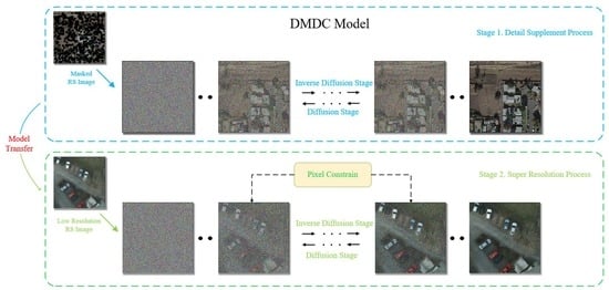
• To the best of our knowledge, we propose a diffusion model with detailed complementary mechanisms for the RSSR task. Different from traditional optimization-based methods, DMDC adopts generation-based methods to enrich image semantics.
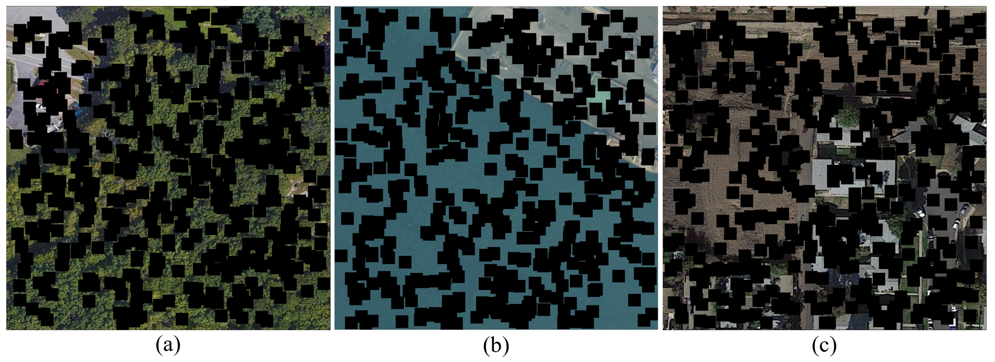
• Aiming at the small and dense characteristics of objects in low-resolution RS images, we propose a detail supplementation task for RSSR for the diffusion model, which achieves accurate detail reconstruction for RSSR tasks.
• To reduce the diversity of DMDC, which may not be suitable for super-resolution tasks, we propose a pixel constraint loss to constrain the inverse diffusion process of the diffusion model.

Extensive comparative experiments demonstrate that our method can achieve superior performance. The rest of the paper is organized as follows: Section 2 gives a brief overview of the work related to DMDC. In Section 3, the Diffusion Model, the Detail Supplement Task, and pixel constraint loss are introduced. Next, in Section 2, we provide detailed information about DMDC and include a detailed experimental analysis of DMDC from both qualitative and quantitative aspects. Finally, the discussion and conclusion are given in Section 5 and Section 6, respectively.

2. Related Work

In this section, we review and discuss RSSR technology and diffusion models which relate to our research.

2.1. Remote Sensing Super Resolution

RSSR refers to the reconstruction of a corresponding HR image from an observed LR image, which helps to improve the effect of high-level remote sensing visual tasks such as segmentation [27,28,29], identification [30], and retrieval [31,32,33]. Most of the traditional RSSR methods adopt an interpolation method, and only reconstruct according to the pixel information of the image itself. However, the quality of the reconstructed image cannot be guaranteed. Recently, deep learning methods have been widely adopted in RSSR technology. Deep learning-based methods can be categorized into four types as mentioned in Section 1: convolution network-based, flow-based, GAN-driven, and PSNR-oriented.

SRCNN [14] can learn linear mappings between images, and extract feature maps of image patches through a simple convolutional network, which improves the reconstruction quality and achieves a fast reasoning speed. However, this method enlarges the target size by an interpolation method, which can’t properly realize end-to-end low-resolution reconstruction. Using convolution structures such as convolution layers or residual networks to extract features directly from LR images greatly improved the efficiency and quality of reconstructions, including FSRCNN [34] and ESPCN [35]. To overcome the problem of fuzzy reconstructed images brought on by the complex and varied RS sampling environment, Tao et al. [36] suggested a deep residual network to optimize the RS image reconstruction process. Although some achievements have been made in the above-mentioned CNN-based high-resolution reconstruction work, due to the complex atmospheric environment, limited spatial resolution, and spectral resolution, remote sensing images are more complex than natural images, which require higher details [37,38]. Luo et al. [39] combined optical flow and deformable convolution, and proposed a Pyramid Flow-Guided Deformable ConvolutionNetwork (Pyramid FG-DCN), with Swin transformer [40] blocks and groups as the main super-resolution backbone. By applying the attention technique to capture the feature variations between channels, Dong et al. [41] overcame the loss of initial features in RSSR reconstruction and enhanced the SR capability of RS images.

Compared with the above methods, the biggest difference and highlight of GAN-driven is the discriminator, which can be trained to discriminate the input generated images. First applying GANs to image SR reconstruction, Ledig et al. [16] proposed a single-image SR reconstruction method using GANs (SRGAN), which optimizes perceptual loss. ESRGAN [42] introduced Residual in Residual Dense Blocks (RRDB) based on SRGAN [16], which further improves the recovered image texture. Subsequently, many ESRGAN-based algorithms [43,44,45] have been improved. ESRGAN+ [43] replaced ESRGAN’s RRDB with RRDRB; [45] used the U-net structure discriminator together to consider both the global and local context of an input image and used GAN and LPIPS [46] loss together for perceptual limit SR. This practice is superior to traditional perception. However, the previous models are based on an optimized way, which relies too much on distorted low-resolution images and is inaccurate in reconstruction. Notably, we manage to use the generation model, which can generate more detailed semantic information of images.

2.2. Diffusion Model

In recent years, research on generative diffusion models has attracted extensive attention. The diffusion model is a generative model driven by non-equilibrium thermodynamics, which can be divided into the forward process and reverse process. To increase the generation effect, Google [17] developed DDPM in 2020, which adopted an autoencoder with the U-Net structure to predict noise and adopted a separate branch network to learn the Gaussian distribution. With a similar purpose, OpenAI [19] proposed a category-guided diffusion model called Guided Diffusion to deepen the network structure of DDPM. The cross-entropy loss between the target categories and the classification score is calculated to determine the gradient. To accomplish the desired generation effect, it merely needs to add guidance during the forward process rather than re-training the diffusion model. However, even if the additional forward network might enhance the effect, the scale of models cannot be further increased due to the huge calculation cost. To solve the issue, Ho et al. [18] employed additional conditional input for the diffusion guidance method without the additional classifiers. Yang et al. [47] integrated the ViT architecture into DDPM, established a direct connection between DDPM and ViT, and introduced a new generative model (GenViT). PDDPM [48] can generate multi-scale images by generating high-resolution images starting from coarser-resolution images using a single-score function trained with positional embeddings. Nair et al. [49] proposed a single image atmospheric turbulence measurement method based on learning, including CNN-based and GAN-based inversion methods, trying to eliminate the distortion in the image. Rombach et al. [50] proposed Latent Diffusion Models (LDMs). Transform diffusion models into powerful and flexible generators for general conditional inputs such as text or bounding boxes, and achieve high resolution in a convolutional fashion rate synthesis. DiffuseVAE [51] integrates VAE [52,53] into the diffusion model framework and uses this framework to design new conditional parameterizations for the diffusion model, effectively equipping the diffusion process with a low-dimensional latent space.

DDPM has completed the task of SR reconstruction in natural scenes, but the related research in RS scenes has not yet been carried out, which is limited by the characteristics of the small targets and complex scenes in RS. We introduce the diffusion model into RSSR for the first time and propose a detail-complementing task to optimize its SR defect for small targets.

3. Methodology

In this section, we introduce the RSSR-based diffusion model in detail and describe the optimization diffusion with a detail supplement. Finally, we further reduce the diversity of DMDC to generate higher-quality images.

3.1. Super Resolution Based Diffusion Model

Image SR aims to recover corresponding HR images from LR images. Typically, an LR image $I_{lr}$ is modeled as the output of the following scaling:

$$I_{lr}=P\left(I_{hr};\varphi \right)$$

(1)

where P is the degradation mapping function and $\varphi$ is a parameter of the degradation process (such as noise distribution parameters or a scaling factor). The researcher needs to recover the HR approximation ${\widehat{I}}_{hr}$ of the real HR image $I_{hr}$ from the LR image $I_{lr}$. Given a dehazing model F, $\omega$ is the parameter representation of the model, and the dehazing process can be expressed as follows:

$${\widehat{I}}_{hr}=F\left(I_{lr};\omega \right)$$

(2)

Image SR reconstruction involves restoring the lost details in the image, i.e., high-frequency information. Traditional SR models usually adopt the end-to-end model architecture for image restoration, which fails to fully understand the information of the whole image. However, reconstruction-based methods can enable the model to fully understand the global characteristics of the image, and restore the entire image from noise. In the past two years, DDPM has shown great potential in image generation and has become an emerging alternative paradigm for generative models, especially when combined with guidance to achieve high fidelity and diversity at the same time.

In this paper, we use the SR model based on diffusion as a general method. The forward and reverse diffusion processes of the diffusion model are essentially the directed graph models parameterized by Markov chains. Diffusion models learn the training data distribution $P\left(x_0\right)$ by performing variational inference on a Markov process with time steps.

As shown in Figure 1, Given an initial data distribution $x_0\sim q\left(x\right)$, a forward diffusion process can be defined. The diffusion process is a process from right to left $X_1,\dots ,X_T$, in which we add spherical Gaussian noise to the clean image in steps of T, producing a series of noisy samples. $X_t$ is obtained by the sum of $X_{t-1}$ and noise, which is only affected by $X_{t-1}$. The step size of each diffusion step is affected by the variable ${\left\{{\beta }_t\in (0,1)\right\}}_{t=1}^T$. In the process of adding noise from $X_{t-1}$ to $X_t$, the $q\left(X_t\mid X_{t-1}\right)$ can be written in the following form, that is, given $X_{t-1}$, $X_t$ obeys the normal distribution with the mean of $\sqrt{1-{\beta }_t}{X}_{t-1}$, and variance of ${\beta }_{t}I$:

$$q\left(X_t\mid X_{t-1}\right)=N\left(X_t;\sqrt{1-{\beta }_t}{X}_{t-1},{\beta }_{t}I\right)$$

(3)

The data sample $X_0$ gradually loses its discernible features as the step size increases. Finally, when $T\to \infty$, $X_t$ is equivalent to an isotropic Gaussian distribution. If the above equation is used to calculate the prior probability distribution of $X_t$, then a total of T sampling is required. We define ${\alpha }_t=1-{\beta }_t$, ${\overline{\alpha }}_t={\prod }_{i=1}^T{\alpha }_i$, then according to the parameter renormalization technique:

$$\begin{array}{cc}\hfill {\mathbf{x}}_t& =\sqrt{{\alpha }_t}{\mathbf{x}}_{t-1}+\sqrt{1-{\alpha }_t}{\mathbf{z}}_{t-1}\hfill \\ & =\sqrt{{\alpha }_t{\alpha }_{t-1}}{\mathbf{x}}_{t-2}+\sqrt{1-{\alpha }_t{\alpha }_{t-1}}{\overline{\mathbf{z}}}_{t-2}\hfill \\ & =\cdots \hfill \\ & =\sqrt{{\overline{\alpha }}_t}{\mathbf{x}}_0+\sqrt{1-{\overline{\alpha }}_t}\mathbf{z}\hfill \end{array}$$

(4)

where ${\mathbf{z}}_{t-1},{\mathbf{z}}_{t-2},\cdots \sim \mathcal{N}(\mathbf{0},\mathbf{I})$ and ${\overline{\mathbf{z}}}_{t-2}$ merges two Gaussians. According to the nature of the Gaussian distribution, we can directly sample $q\left(x_t\mid x_0\right)$ to obtain the prior conditional probability distribution of $X_0$ at each time step.

$$\begin{array}{cc}q\left(x_t\mid x_0\right)& =\mathcal{N}\left(x_t;\sqrt{{\overline{\alpha }}_t}{x}_0,\left(1-{\overline{\alpha }}_t\right)\mathbf{I}\right)\hfill \\ & =\sqrt{{\overline{\alpha }}_t}{x}_0+ϵ\sqrt{1-{\overline{\alpha }}_t},ϵ\sim \mathcal{N}(\mathbf{0},\mathbf{I})\end{array}$$

(5)

Combining the above two formulas, the joint posterior distribution of $X_{t-1}$ about $X_t$ and $X_0$ can be obtained. If we want to sample a $X_0$, we can first iterate gradually from the noise-saturated $X_T$ until back to $X_0$. Assume that we can construct a sequence with $q\left(x_t\mid x_0\right)$, then the random noise can be reversed to the image distribution through the reverse Markov process. Therefore, the aim of the diffusion model is to find a distribution similar to $q\left(x_{t-1}\mid x_t,x_0\right)$.

The denoising process is the opposite of the noise addition process. A noise sample is sampled from the standard normal distribution, and then gradually denoised to obtain a sample in the data distribution. We model this denoising process with a neural network to predict the parameters of the Gaussian distribution ${\mu }_{\theta }\left({\mathbf{x}}_t,t\right)$ and ${\Sigma }_{\theta }\left({\mathbf{x}}_t,t\right)$:

$$p_{\theta }\left({\mathbf{x}}_{t-1}\mid {\mathbf{x}}_t\right)=\mathcal{N}\left({\mathbf{x}}_{t-1};{\mathit{\mu }}_{\theta }\left({\mathbf{x}}_t,t\right),{\Sigma }_{\theta }\left({\mathbf{x}}_t,t\right)\right)$$

(6)

$$p_{\theta }\left({\mathbf{x}}_{0:T}\right)=p\left({\mathbf{x}}_T\right)\prod _{t=1}^T{p}_{\theta }\left({\mathbf{x}}_{t-1}\mid {\mathbf{x}}_t\right)$$

(7)

Although $p_{\theta }\left(x_{t-1}\mid x_t\right)$ cannot be expressed explicitly, $p_{\theta }\left(x_{t-1}\mid x_t,x_0\right)$ can expressed in formula:

$$q\left(x_{t-1}\mid x_t,x_0\right)=\mathcal{N}\left(x_{t-1};\overline{\mu }\left(x_t,x_0\right),{\overline{\beta }}_{t}I\right)$$

(8)

$${\overline{\beta }}_t=\frac{1}{\frac{{\alpha }_t}{{\beta }_t}+\frac{1}{1-{\overline{\alpha }}_{t-1}}}=\frac{1-{\overline{\alpha }}_{t-1}}{1-{\overline{\alpha }}_t}{\beta }_t$$

(9)

$${\mathit{\mu }}_{\theta }\left({\mathbf{x}}_t,t\right)=\frac{1}{\sqrt{{\alpha }_t}}\left(x_t-\frac{{\beta }_t}{\sqrt{1-{\overline{\alpha }}_t}}{z}_t\right)$$

(10)

For two single-variable Gaussian distributions p and q, their KL divergence satisfies:

$$KL(p,q)=log\frac{{\sigma }_2}{{\sigma }_1}+\frac{{\sigma }_1^2+{\left({\mu }_1-{\mu }_2\right)}^2}{2{\sigma }_2^2}-\frac{1}{2}$$

(11)

q is a known partial Gaussian distribution, and p is the distribution to be fitted. Since it is assumed that p variance ${\sigma }_t$ is constant, we only need to approximate the mean of p and q. Equivalent to the minimization formula:

$$Loss={\mathbb{E}}_q\left(\frac{1}{2{\sigma }_t^2}{∥{\overline{\mu }}_t\left(x_t,x_0\right)-{\mu }_{\theta }\left(x_t,t\right)∥}^2\right)+C$$

(12)

$x_t$ is a variable determined by $x_0$ and noise $ϵ$. Ho et al. [18] found during training that removing the coefficients before Loss can stabilize the training. The simplified loss is:

$$\mathrm{Loss}={\mathbb{E}}_{x_0,ϵ}\left({∥ϵ-ϵ\theta \left(\sqrt{{\overline{\alpha }}_t}{x}_0+\sqrt{1-{\overline{\alpha }}_t}ϵ,t\right)∥}^2\right)$$

(13)

The mean ${\mu }_{\theta }\left({\mathbf{y}}_t,x,t\right)$ is estimated according to,

$${\mu }_{\theta }\left({\mathbf{y}}_t,x,t\right)=\frac{1}{\sqrt{\left(1-{\beta }_t\right)}}\left(y_t-\frac{{\beta }_t}{\sqrt{1-{\overline{\alpha }}_t}}{ϵ}_{\theta }\left(x,y_t,t\right)\right)$$

(14)

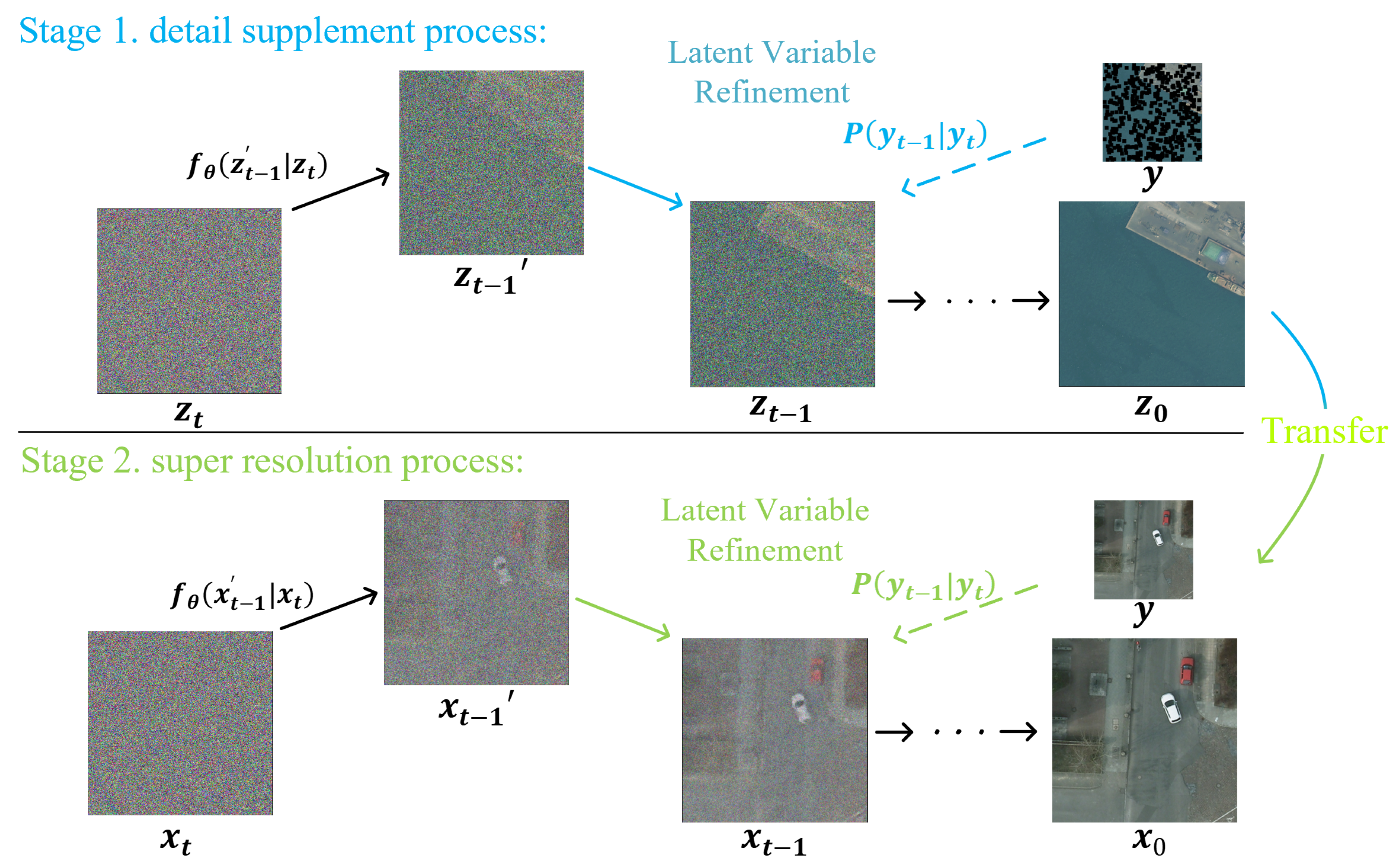
3.2. Optimizing Diffusion with Detail Complement

The diffusion model has achieved great success in natural scenes, but some problems have emerged when applied to RS scenes. SR needs to acquire the texture of the target domain while retaining the structure of the input images. SR targets in natural scenes tend to be of a single type and have large granularity. For example, face image SR often has only one face in a picture, which has a single distribution and is easy to recover. Different from traditional scenes, the granularity of targets in RS images is complex, which makes the diffusion models unable to recover target details with more information. The small granularity of the object makes it difficult for the model to capture the high-frequency information in the object at LR. To make the diffusion model obtain sufficient reconstruction ability of complex scenes, we set up a detail supplementation task to make it have a powerful feature repair ability.

The diffusion model with detail complement can obtain the sensing of RS images by recovering most of the occluded areas, which can pay more attention to LR small targets in RS images. Specifically, we randomly mask most of the information in the image and only provide some areas for model reconstruction. As shown in Figure 2, the mask part consists of r randomly distributed patches with the size of $m\times n$, which is similar to small and dense objects in RS images. By recovering these obscured patches, the model improves the perception and reconstruction of small objects. We define the diffusion model as f, $\theta$ is the parameter representation of the model, $Mas{k}_{r,m\times n}\left(Z\right)$ is the masked RS image. By minimizing the loss through gradient descent, the detail completion process can be expressed as:

$$\begin{array}{c}\hfill Los{s}_{dc}={\nabla }_{\theta }{∥f_{\theta }\left(Mas{k}_{r,m\times n}\left(Z\right),\sqrt{\eta }{\mathit{y}}_0+\sqrt{1-\eta }ϵ,\eta \right)-ϵ∥}_p^p\end{array}$$

(15)

The masked patches have the characteristics of small size and high density, which is also in line with the characteristics of small object granularity in RS images. The model learns more small-grained information about the RS image through these mask squares. The diffusion model with detail complement is then used as our optimization super-resolution model. Under the training weight of detail complement task, DMDC can pay more attention to the details in LR images and improve the reconstruction ability of small targets.

3.3. Pixel Constraint Loss

The reverse diffusion process of the model is random and varied. Combined with subtle targets in remote sensing scenes, pixel-level constraints can guide the diffusion process to achieve a more refined SR reconstruction. Therefore, we propose the pixel constraint loss to further reduce the gap with HR images. The pixel constraint loss component improves the overall accuracy of the constructed image, i.e., the pixel values are directly consistent with the original image while maintaining the same lighting and contrast as the original HR image. Specific to each training example, Y is the original HR image. X is reconstructed from the LR image, which has a height of H and a width of W. The pixel constraint loss specific calculation formula is as follows:

$$Los{s}_{pixels}=\frac{{\sum }_{x=1}^W{\sum }_{y=1}^H\left(\left|Y_{i,j}-X_{i,j}\right|\right)}{WH}$$

(16)

Notably, the pixel constraint loss is used in the DMDC training process. The pixel constraint loss method achieves accurate generation by limiting the inverse diffusion process of the diffusion model, thereby further optimizing the RSSR. The complete inference procedure of DMDC is given in Algorithms 1 and 2.

Algorithm 1 Training a DMDC model $f_{\theta }$

1: Input: $\left(\mathit{x},{\mathit{y}}_0\right)\sim p(\mathit{x},\mathit{y})$,

$\eta \sim p\left(\eta \right)$,

$ϵ\sim \mathcal{N}(\mathbf{0},\mathbf{I})$

2: repeat;

3: Train diffusion model for detail supplement

${\nabla }_{\theta }{∥f_{\theta }\left({Mask}_{r,m\times n}\left(Z\right),\sqrt{\eta }{\mathit{y}}_0+\sqrt{1-\eta }ϵ,\eta \right)-ϵ∥}_p^p$

4: Take a gradient descent step on ${\nabla }_{\theta }{∥f_{\theta }\left(\mathit{x},\sqrt{\eta }{\mathit{y}}_0+\sqrt{1-\eta }ϵ,\eta \right)-ϵ∥}_p^p$

$+\frac{{\sum }_{x=1}^W{\sum }_{y=1}^H\left(\left|y_{0_{i,j}}-f_{\theta }\left(\mathit{x},\sqrt{\eta }{\mathit{y}}_0+\sqrt{1-\eta }ϵ,\eta \right)\right|\right)}{WH}$

5: until converged

6: return: $f_{\theta }$

Algorithm 2 Inference in T iterative refinement steps

1: Input: ${\mathit{y}}_T\sim \mathcal{N}(\mathbf{0},\mathbf{I})$

$f_{\theta }$

2: for $t=T,\dots ,1$ do

3: $\mathit{z}\sim \mathcal{N}(\mathbf{0},\mathbf{I})$ if $t>1$, else $\mathit{z}=\mathbf{0}$

4: $ϵ\sim \mathcal{N}(\mathbf{0},\mathbf{I})$

5:   ${\mathit{y}}_{t-1}=\frac{1}{\sqrt{{\alpha }_t}}\left({\mathit{y}}_t-\frac{1-{\alpha }_t}{\sqrt{1-{\eta }_t}}{f}_{\theta }\left(\mathit{x},{\mathit{y}}_t,{\eta }_t\right)\right)+\sqrt{1-{\alpha }_t}\mathit{z}$

6: end for

7: return $y_0$

4. Results and Analysis

In this section, we first introduce the dataset, evaluation metrics, and experimental details. Then, we exhibit the generation effect of DMDC. Furthermore, we conduct extensive ablation experiments to systematically compare the performance of the DMDC models. Finally, the visual experiments and evaluation metrics are compared.

4.1. Data Set and Evaluation Metrics

4.1.1. Data Set

We choose the extremely challenging Potsdam (Germany) dataset and Vaihingen (Germany) dataset proposed by the International Society for Photogrammetry and Remote Sensing (ISPRS). 38 RS images with a spatial resolution of 5 cm are collected in Potsdam, a historic city. Each image with 6000 × 6000 pixels is composed of three channels: red (R), green (G), and blue (B). This dataset includes the six most common types of land cover (impermeable surface, buildings, low vegetation, trees, cars, and clutter). In this paper, we follow the train-test split scheme in most existing works [54], and select 14 images as the test set, and 5 images as the verification set. The remaining images are utilized to train our models. As shown in Figure 3, after cutting and sampling, each sample in the above dataset contains images with different resolutions: 64 × 64, 128 × 128, 256 × 256, and 512 × 512. Furthermore, when performing the detailed supplement task, we choose the FAIR dataset [55] to enhance the small target SR ability of the model. Finally, we test the DMDC directly on the Vaihingen dataset without any fine-tuning operation to demonstrate the generalization ability of our DMDC model.

4.1.2. Evaluation Metrics

We adopt the Image Quality Assessment (IQA) method with reference and IQA no-reference as evaluation metrics to evaluate the model more comprehensively and accurately, i.e., Peak Signal-to-Noise Ratio (PSNR) [11], Structural Similarity (SSIM) [56] and BRISQUE [57]. PSNR represents the ratio between the maximum possible power of a signal and the power of corrupting noise that affects the fidelity of its representation. SSIM [56] focuses on measuring the correlation of adjacent pixels in digital images, reflecting the structural information of objects in real scenes, closer to human vision. SSIM [56] mainly considers three key characteristics of the image: luminance, contrast, and structure, which are mathematically defined as follows:

$$luminance(x,y)=\frac{2{\xi }_x{\xi }_y+{\alpha }_1}{{\xi }_x^2+{\xi }_y^2+{\alpha }_1}$$

(17)

$$contrast(x,y)=\frac{2{\zeta }_{xy}+{\alpha }_2}{{\sigma }_x^2+{\sigma }_y^2+{\alpha }_2}$$

(18)

$$structure(x,y)=\frac{{\sigma }_{xy}+{\alpha }_3}{{\sigma }_x{\sigma }_y+{\alpha }_3}$$

(19)

where ${\xi }_x$ and ${\xi }_y$ represent the mean of $x,y$ respectively, ${\sigma }_x$ and ${\sigma }_y$ represent the standard deviation of $x,y$ respectively. ${\sigma }_{xy}$ represents the covariance of x and y. And ${\alpha }_1,{\alpha }_2,{\alpha }_3$ are constants, respectively. In actual engineering calculations, we generally set $\alpha =\beta =\gamma =1$, and ${\alpha }_3={\alpha }_2/2$, SSIM can be simplified as follows:

$$SSIM(x,y)=\frac{\left(2{\xi }_x{\xi }_y+{\alpha }_1\right)\left({\sigma }_{xy}+{\alpha }_2\right)}{\left({\xi }_x^2+{\xi }_y^2+{\alpha }_1\right)\left({\sigma }_x^2+{\sigma }_y^2+{\alpha }_2\right)}$$

(20)

BRISQUE [57] is a reference-free spatial domain IQA algorithm. The overall principle of the algorithm is to extract mean subtracted contrast normalized (MSCN) coefficients from the image, fit the MSCN coefficients to an asymmetric generalized Gaussian distribution (AGGD), extract the features of the fitted Gaussian distribution, and input them into the support vector machine (SVM), thereby obtaining an IQA result. The MSCN coefficient $\widehat{I}(i,j)$ is defined as:

$$\widehat{I}(i,j)=\frac{I(i,j)-\mu (i,j)}{\sigma (i,j)+C}$$

(21)

$$\mu (i,j)=\sum _{k=-K}^K\sum _{l=-L}^L{w}_{k,l}{I}_{k,l}(i,j)$$

(22)

$$\sigma (i,j)=\sqrt{\sum _{k=-K}^K\sum _{l=-L}^L{w}_{k,l}{\left(I_{k,l}(i,j)-\mu (i,j)\right)}^2}$$

(23)

where $u(x,y)$ is the result after Gaussian filtering, and $\sigma (x,y)$ is the standard deviation. MSCN has no strong dependence on texture. Therefore, the extracted features are more applicable. The definition of generalized Gaussian distribution GGD:

$$f\left(x;\alpha ,{\sigma }^2\right)=\frac{\alpha }{2\beta \Gamma (1/\alpha )}exp\left(-{\left(\frac{\left|x\right|}{\beta }\right)}^{\alpha }\right)$$

(24)

$$\beta =\sigma \sqrt{\frac{\Gamma (1/\alpha )}{\Gamma (3/\alpha )}}$$

(25)

and $\Gamma (·)$ is the Gamma function:

$$\Gamma \left(a\right)={\int }_0^{\infty }{t}^{a-1}{e}^{-t}dta>0$$

(26)

By observing that the local normalized luminance coefficients (MSCN) of natural images strongly tend to be unit normal Gaussians, we assume that distortion will change the distribution of MSCN, and extract features based on this.

4.2. Implementation Details

We perform all experiments on three NVIDIA RTX 3090 GPUs. We crop the images to 512 × 512 and convert them to LR images of 64 × 64, 128 × 128, 256 × 256 for the ×8, ×4, ×2 SR task. A series of operations for data augmentation (such as rotation, flip, etc.) are carried out simultaneously to improve the robustness of the model. We followed [21] model structure for SR reconstruction in natural scenes. First, supplement the details with the FAIR dataset, and train 200,000 iterations. We performed 1M training steps for all DMDC and regression models with a batch size of 8. 2000 denoising steps are used in DMDC, where ${\beta }_t$ is set from $2\times {10}^4$ to $1\times {10}^2$. Consistent with [21], we use a fixed learning rate of $1\times {10}^4$ for the DMDC model and $1\times {10}^5$ for the regression model, followed by a linear warm-up schedule with Adam optimizer and over 1,000,000 training steps. For each set of experiments, we perform the same training and validation five times, and obtain an average result to make the experiments more convincing.

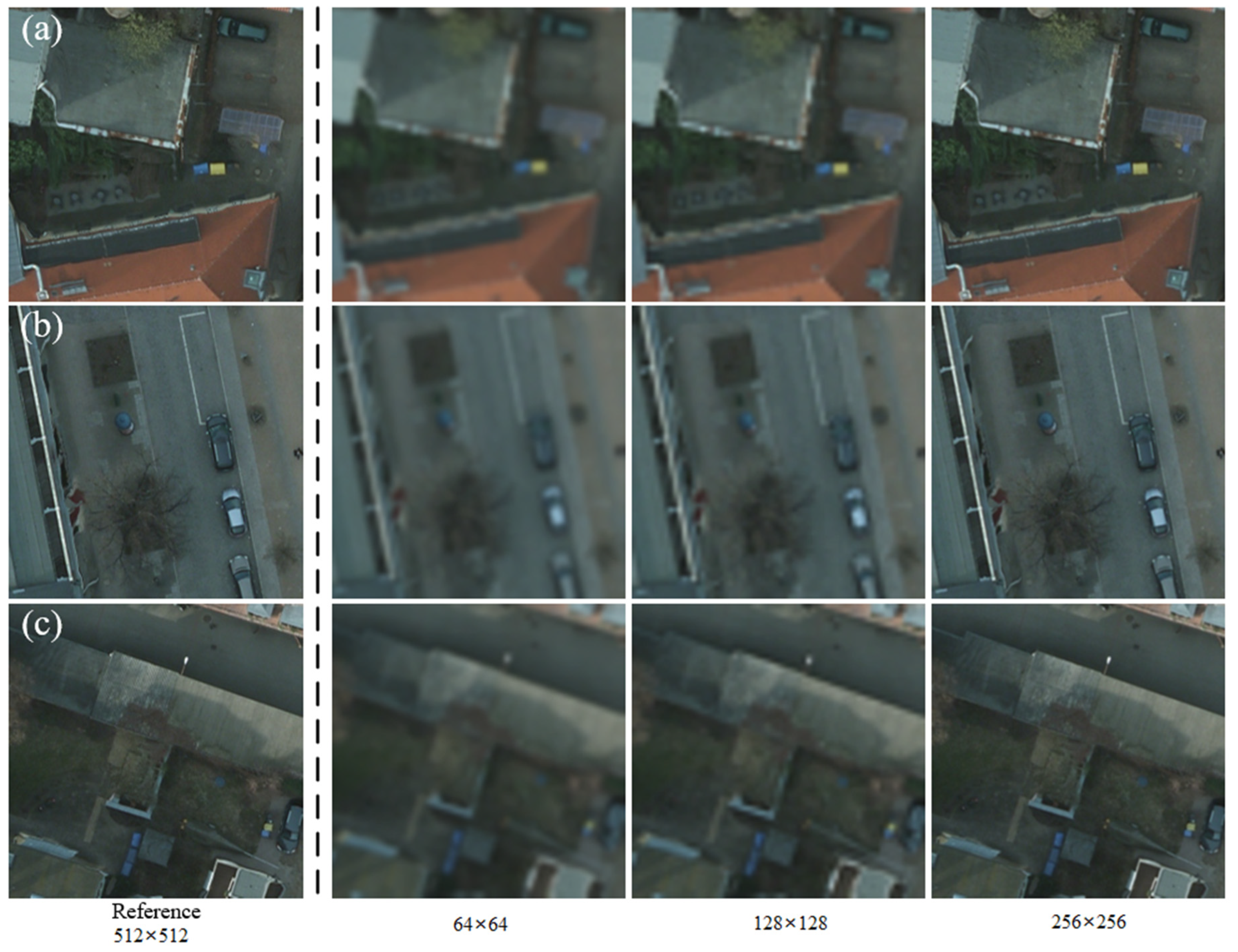
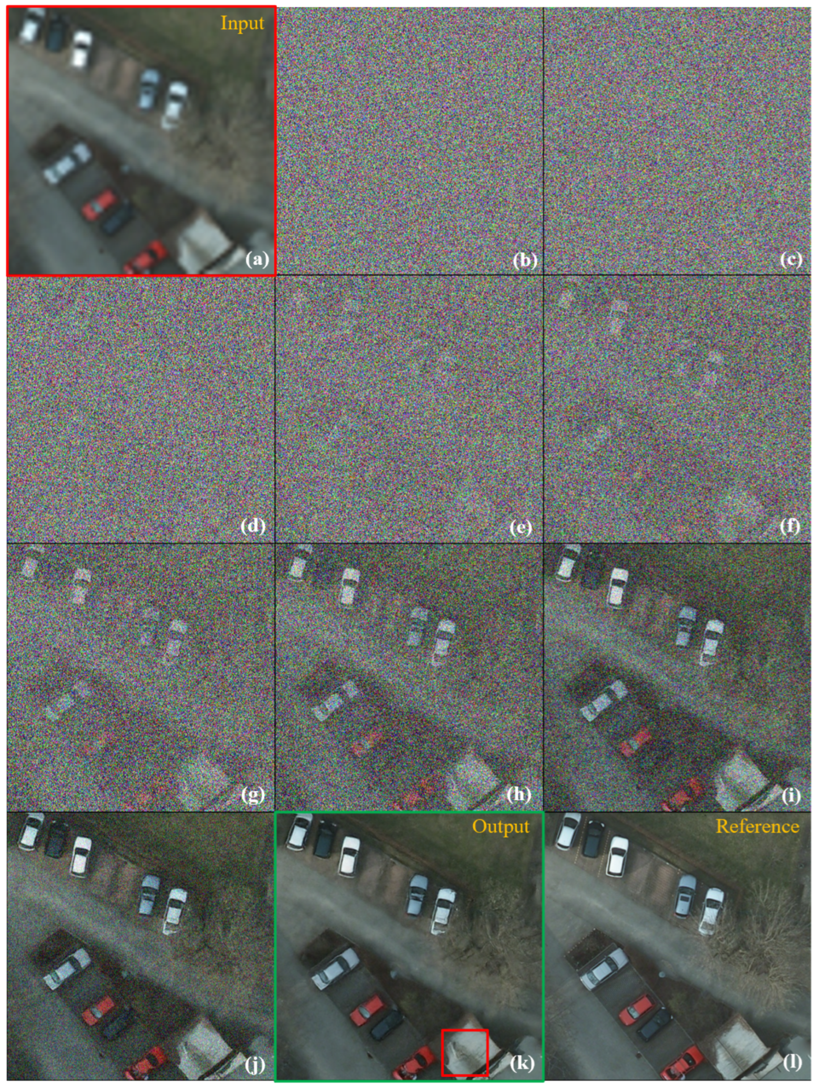
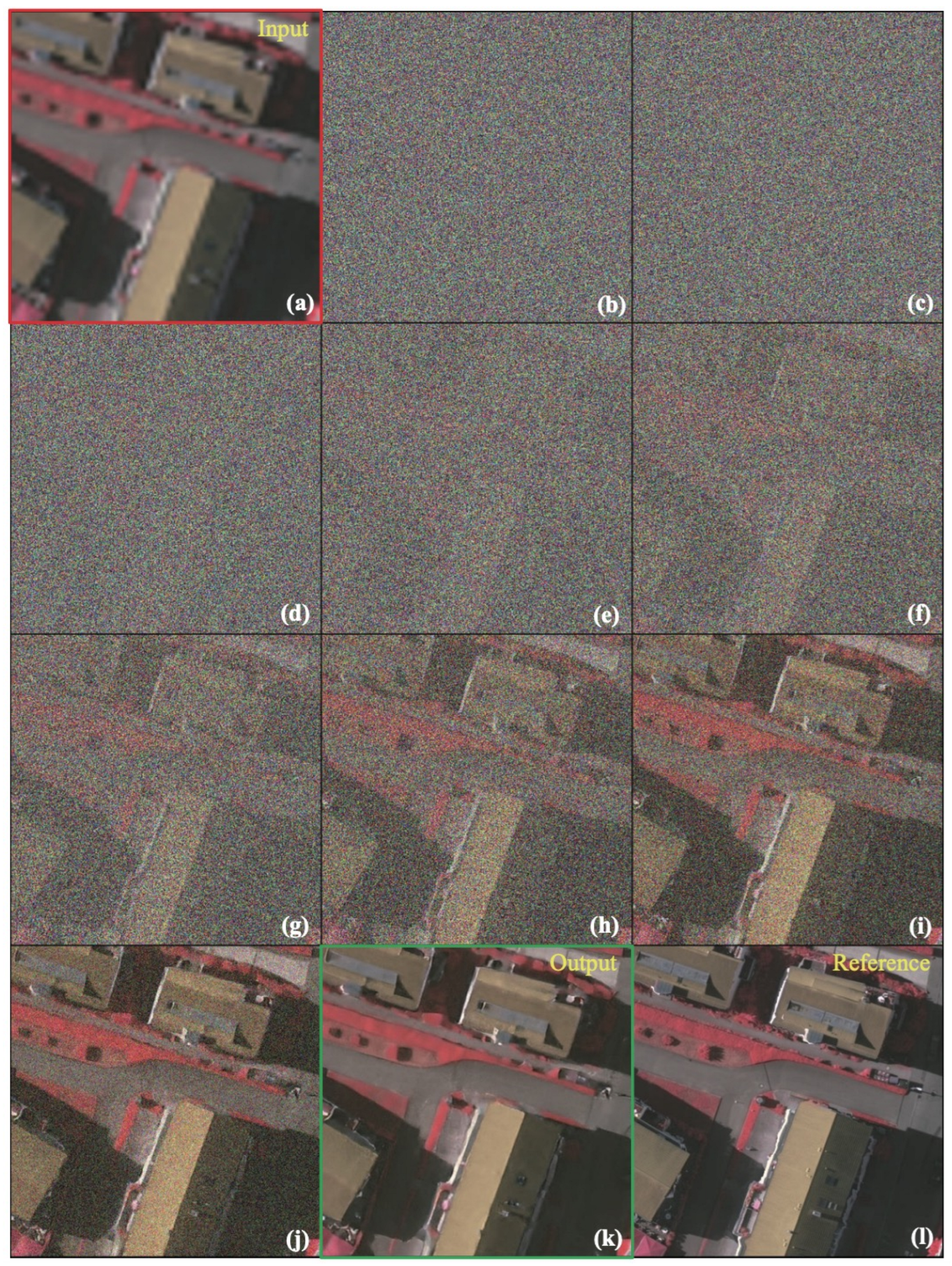
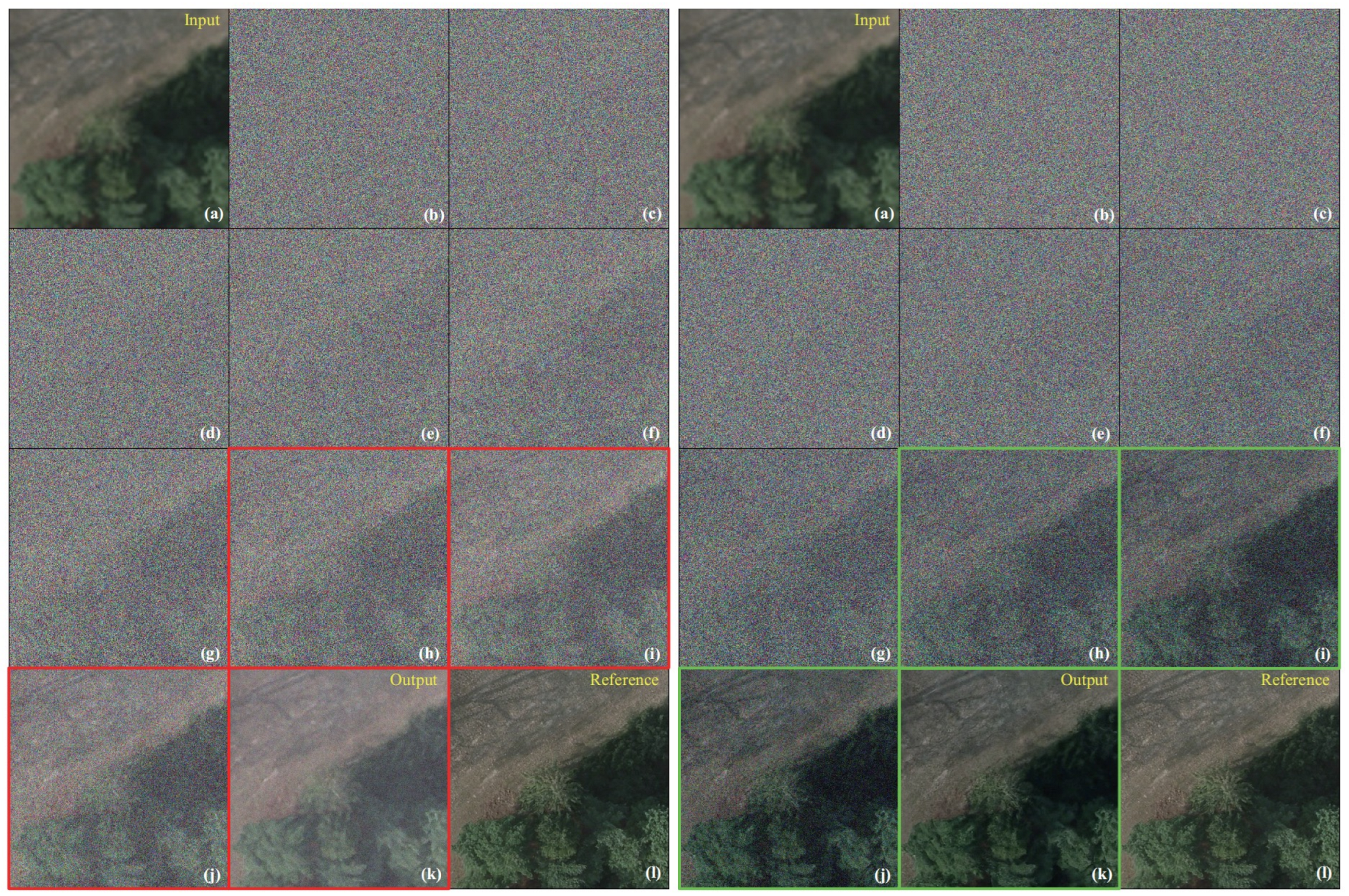
4.3. Generate Visualization

4.3.1. Detail Supplement Visualization

Figure 4 shows the visualization of our DMDC optimization process for small targets in RS images. We can observe that even after most of the image details are covered, DMDC can still generate RS HR images with rich semantic information from very little context information. As can be seen from Figure 4a,b, our model can reconstruct the semantic information in the source image, which is masked by a large area. In Figure 4c, the model also has a strong generation ability in the dense scene of small targets.

4.3.2. Visualization on Potsdam

Figure 5 shows our process of generating a 512 × 512 HR image from a 64 × 64 LR image, where the input Figure 5a is our initial LR image, and under its guidance, DMDC gradually restores a 512 × 512 high-definition image Figure 5k from the randomly generated noise Figure 5b. By comparing with our label results Figure 5l, it can be seen that the model has a high restoration similarity to the image with very little noise. In particular, the contrasting roads, cars, and grasslands in the picture can be reproduced clearly. At the same time, our network takes contextual information in the image into consideration, so it can distinguish roads from similar targets, such as dirt roads and parking spaces. The fly in the ointment is that the clarity of the lower right corner of the picture is not restored enough. This is mainly because the definition of the reference image is insufficient, which leads to the degradation of image quality.

4.3.3. Visualization on Vaihingen

Unlike Potsdam, Vaihingen was shot in the center of the city, featuring dense and complex historical buildings, roads, and trees, which made SR reconstruction more challenging. In addition, the color distribution of the two datasets is also very different. Figure 6 shows the visual SR generation results of our model directly migrated to the Vaihingen dataset. Without any fine-tuning for this dataset, our DMDC can still achieve a high-quality super-resolution reconstruction of Vaihingen, and can recover most of the details in the image (including roof details and dense trees). The test on the Vaihingen dataset proves that the detail supplement task can improve the super-resolution reconstruction ability of DMDC for small targets. At the same time, the method of direct migration shows that DMDC has strong generalization ability.

4.4. Effective of Pixel Constraint Loss

To evaluate the effectiveness of our proposed pixel constraint loss, we conduct ablation studies using DMDC models with and without pixel constraints. Figure 7 visualizes the whole process of DMDC super-resolution reconstruction for two sets of different configurations on the Potsdam dataset. On the one hand, the reconstruction of DMDC is more efficient and purposeful after using pixel constraint loss to generate constraints on DMDC. Starting from Figure 7h, the DMDC model using the pixel constraint has preliminarily reconstructed the color and texture information of the HR image, while the one without the pixel constraint is blurry. On the other hand, from the final reconstruction result Figure 7k, adding the pixel constraint enables DMDC to generate HR images with balanced tones and more detailed textures. This ablation study demonstrates the important contribution of pixel constraint.

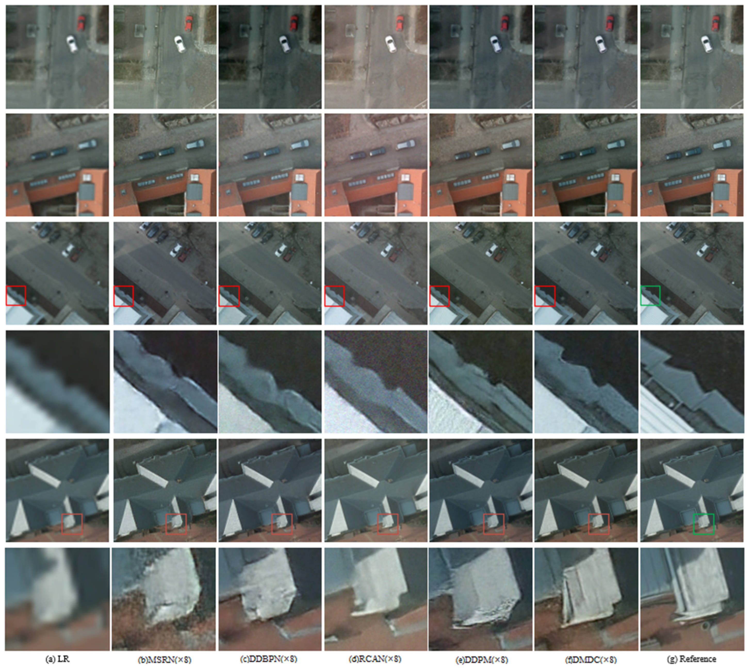
4.5. Comparison with State-of-the-Art

We conduct extensive experiments on SR of RS images, compare them with SOTA solutions, and perform ablation analysis. We compare DMDC with MSRN [58], DDBPN [59], RCAN [60], DDPM [18]. Figure 8 shows the qualitative results of each model on the ISPRS-Potsdam dataset. It can be seen that the images generated by the baseline regression model are faithful to the input, but fuzzy and lacking in details. In contrast, for remote sensing images with multiple targets, the images generated by DMDC have rich details and sharp edges, well-balanced naturalness and sharpness, and produce strong consistency with LR images. Specifically, the red box in Figure 8 shows the SR reconstruction ability in details of DMDC for the edge of the house, with the smallest gap with the reference image.

As shown in

Table 1. Super-resolution results of ×8, ×4, ×2 magnification on ISPRS Potsdam and Vaihingen datasets. We report quantitative results for the SSIM and BRISQUE metrics. Note that we trained and tested on Potsdam. Then it is directly transferred to Vaihingen for testing, without any training or fine-tuning.

	Dataset	×8 (Scale)			×4 (Scale)			×2 (Scale)
		PSNR↑	SSIM↑	BRISQUE↓	PSNR↑	SSIMred↑	BRISQUE↓	PSNR↑	SSIM↑	BRISQUE↓
Bicubic	Potsdam Testset	25.68	0.6953	32.1548	28.21	0.7625	30.1589	32.31	0.8746	28.6751
EDSR [61]		25.85	0.6987	27.1245	28.32	0.7649	26.6271	32.58	0.8789	25.3897
MSRN [58]		25.48	0.7023	26.7856	28.29	0.7713	26.6857	32.21	0.8803	25.8921
DDBPN [59]		25.52	0.7049	24.3217	27.32	0.7725	23.8912	32.02	0.8934	24.3259
RCAN [60]		25.92	0.7056	25.6812	28.02	0.7756	24.8934	33.14	0.9012	22.3487
DDPM [18]		25.98	0.7173	23.3415	27.86	0.7832	22.1258	32.12	0.9074	20.3274
DMDC (ours)		25.34	0.7329	22.9012	28.12	0.7869	20.1645	32.87	0.9123	19.5632
Driectly Transfer
Bicubic	Vaihingen Testset	20.36	0.5632	28.1567	23.21	0.7089	26.3489	27.73	0.8324	24.8948
EDSR [61]		22.24	0.5806	26.3179	24.31	0.7205	23.4986	27.96	0.8315	22.3472
MSRN [58]		21.25	0.5749	25.5741	23.98	0.7194	22.5914	27.48	0.8417	21.8798
DDBPN [59]		21.29	0.5864	25.3287	25.12	0.721	22.5324	28.07	0.8397	21.5714
RCAN [60]		22.34	0.5876	23.5786	24.32	0.7231	21.8649	28.13	0.8423	20.6819
DDPM [18]		22.17	0.6427	17.8547	25.02	0.7596	17.2684	27.63	0.8869	16.6817
DMDC (ours)		23.46	0.6696	16.6959	25.79	0.7627	15.9487	28.24	0.8975	15.3271

, we provide quantitative results on (×8, ×4, ×2 scale) SR tasks, which outperform other methods by 1 to 3 points. We utilize the Structural Similarity Index (SSIM) to compare methods. Furthermore, we report no-reference image quality assessments in the spatial domain for all methods. DMDC achieves the best evaluation scores among the {64 × 64, 128 × 128, 256 × 256 → 512 × 512 resolution} models, implying the best super-resolution reconstruction performance among the considered SR methods. In particular, we directly transfer the model trained on the Potsdam dataset to the Vaihingen dataset for (×8, ×4, ×2 scale) testing, without any fine-tuning. Quantitative results on the Vaihingen dataset demonstrate that DMDC can still maintain superior performance when the data distribution changes. Overall, our proposed DMDC achieves the highest fidelity and naturalness among all these methods. Meanwhile, the DMDC model with pixel constraint loss has stronger generalization than other models. Meanwhile, the PSNR evaluation metric is discussed in the last part of the experiment.

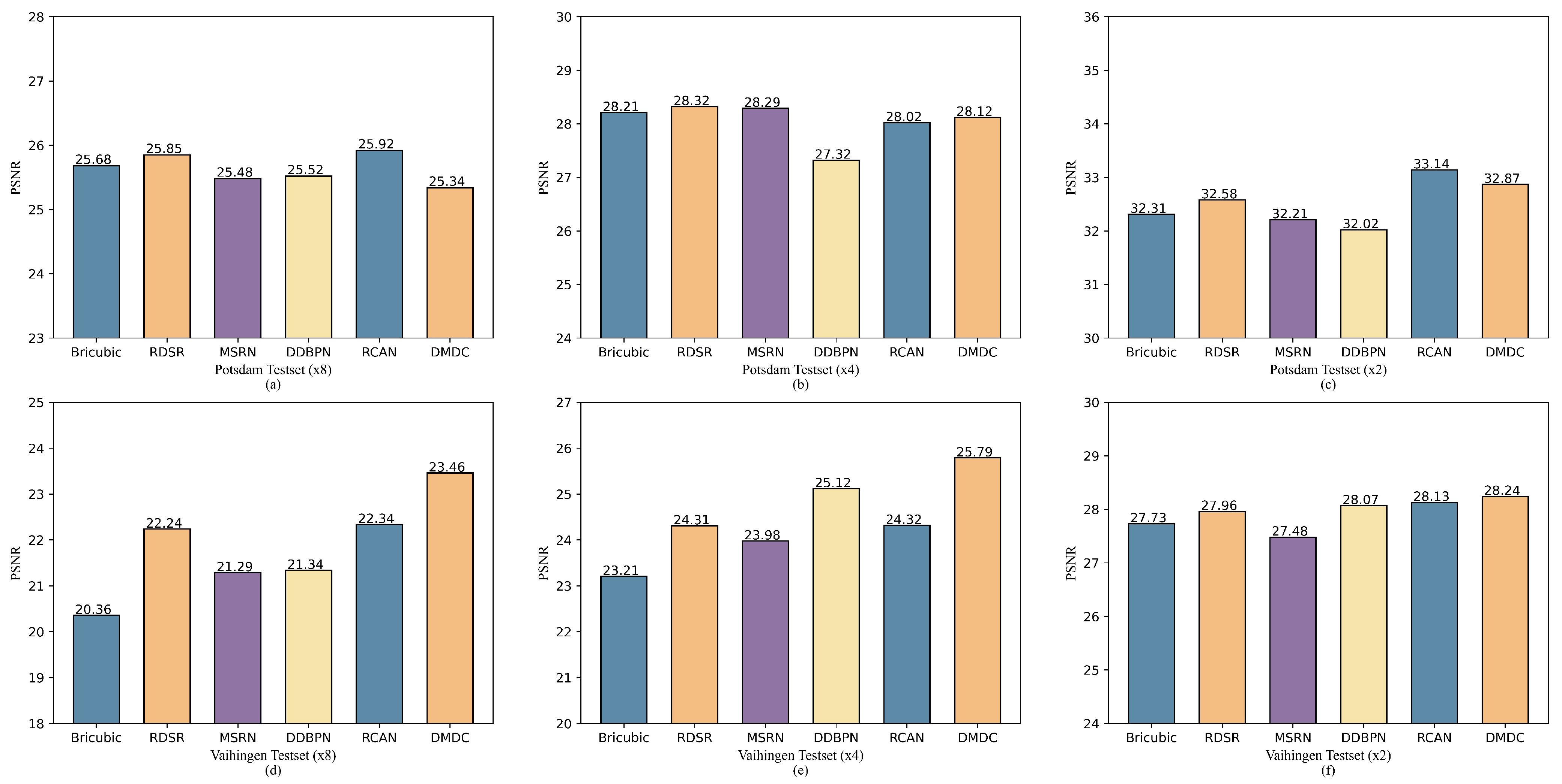
4.6. Discussion of DMDC on PSNR Indicator

As shown in Figure 9, we perform the super-resolution task of ×8, ×4, ×2 magnifications on the Potsdam and Vaihingen test datasets and report their PSNR quantitative results. We observe that on the Potsdam dataset, DMDC is basically on par with other methods. This is because PSNR is a strict metric that only measures the reference value of image quality between maximum signal and background noise, which has limitations. On the Potsdam test set, the CNN-based end-to-end method has a stronger fitting ability, and this overfitting ability recovers the image from the pixel level. Therefore CNN-based methods strictly follow the correspondence of the PSNR evaluation metric, resulting in higher scores on the test set with the same distribution.

While our method is based on a generative model, it does not strictly follow the correspondence of PSNR evaluations. This results in an unremarkable PSNR of DMDC on the Potsdam test set. However, our method outperforms other methods on the PSNR metric when they are both transferred to the Vaihingen test set. This demonstrates the shortcomings of pixel-level fitting of CNN-based methods and also demonstrates that our method has a strong generalization ability. When the magnification is 8 or 4, the generalization of the model transfer is more significant, and when the magnification is 2, the gap of the model in the transfer performance gradually narrows. In addition, DMDC pays more attention to the higher perceived quality of vision and its relevance to human perception.

5. Discussion

DMDC achieves super-resolution reconstruction through iterative thinning, which can generate clear, highly detailed, and semantic images. Compared with other methods, DMDC only imitates the reverse process corresponding to a simple forward process, thus avoiding the over-smoothing problem caused by multiple convolutions in the CNN-based method and the mode collapse problem caused by unstable training in the GAN-based method. Furthermore, pixel constraint loss can guide the generation process of DMDC to generate more stable and high-quality images. In the future, we will further develop our work in two areas. On the one hand, we will work on speeding up the DDPM optimization process to make it more suitable for real-time applications. On the other hand, we will design state embeddings that are more in line with remote sensing properties to further improve RSSR capabilities.

6. Conclusions

This paper presents a diffusion model with a detailed complementary mechanism. Within the scope of our knowledge, we take the lead in implementing the remote sensing super-resolution task based on the diffusion model, which may become a new paradigm for generative models in the field of remote sensing super-resolution. Aiming at the difficulty of super-resolution reconstruction of small objects and dense objects in remote sensing images, we propose an optimized detail supplementation mechanism to enable the model to have the capability of detail super-resolution reconstruction. Furthermore, considering that the randomness in the diffusion model generation process is not conducive to super-resolution reconstruction, we introduce a pixel constraint loss to guide the reconstruction of DMDC, which can speed up the convergence and stabilize the training. Extensive experiments verify the superior performance and strong generalization ability of our method on the task of remote sensing image super-resolution. DMDC is also a strong candidate for improving performance on high-level visual tasks.

References

1. Dong, R.; Zhang, L.; Fu, H. RRSGAN: Reference-based super-resolution for remote sensing image. IEEE Trans. Geosci. Remote Sens. 2021, 60, 1–17. [Google Scholar] [CrossRef]
2. Zhang, X.g. A new kind of super-resolution reconstruction algorithm based on the ICM and the bicubic interpolation. In Proceedings of the 2008 International Symposium on Intelligent Information Technology Application Workshops, Shanghai, China, 21–22 December 2008; pp. 817–820. [Google Scholar]
3. Zhang, X.g. A new kind of super-resolution reconstruction algorithm based on the ICM and the bilinear interpolation. In Proceedings of the 2008 International Seminar on Future BioMedical Information Engineering, Wuhan, China, 18 December 2008; pp. 183–186. [Google Scholar]
4. Begin, I.; Ferrie, F. Blind super-resolution using a learning-based approach. In Proceedings of the ICPR 2004: 17th International Conference on Pattern Recognition, Cambridge, UK, 26 August 2004; Volume 2, pp. 85–89. [Google Scholar]
5. Joshi, M.V.; Chaudhuri, S.; Panuganti, R. A learning-based method for image super-resolution from zoomed observations. IEEE Trans. Syst. Man Cybern. Part B 2005, 35, 527–537. [Google Scholar] [CrossRef] [PubMed]
6. Chan, T.M.; Zhang, J. An improved super-resolution with manifold learning and histogram matching. In International Conference on Biometrics; Springer: Berlin/Heidelberg, Germany, 2006; pp. 756–762. [Google Scholar]
7. Ran, Q.; Xu, X.; Zhao, S.; Li, W.; Du, Q. Remote sensing images super-resolution with deep convolution networks. Multimed. Tools Appl. 2020, 79, 8985–9001. [Google Scholar] [CrossRef]
8. Zhu, Y.; Geiß, C.; So, E. Image super-resolution with dense-sampling residual channel-spatial attention networks for multi-temporal remote sensing image classification. Int. J. Appl. Earth Obs. Geoinf. 2021, 104, 102543. [Google Scholar] [CrossRef]
9. Ibrahim, M.R.; Benavente, R.; Lumbreras, F.; Ponsa, D. 3DRRDB: Super Resolution of Multiple Remote Sensing Images Using 3D Residual in Residual Dense Blocks. In Proceedings of the IEEE/CVF Conference on Computer Vision and Pattern Recognition, New Orleans, LA, USA, 19–20 June 2022; pp. 323–332. [Google Scholar]
10. Jiang, K.; Wang, Z.; Yi, P.; Wang, G.; Lu, T.; Jiang, J. Edge-enhanced GAN for remote sensing image superresolution. IEEE Trans. Geosci. Remote Sens. 2019, 57, 5799–5812. [Google Scholar] [CrossRef]
11. Xiong, Y.; Guo, S.; Chen, J.; Deng, X.; Sun, L.; Zheng, X.; Xu, W. Improved SRGAN for remote sensing image super-resolution across locations and sensors. Remote Sens. 2020, 12, 1263. [Google Scholar] [CrossRef]
12. Li, F.; Jia, X.; Fraser, D. Universal HMT based super resolution for remote sensing images. In Proceedings of the 2008 15th IEEE International Conference on Image Processing, San Diego, CA, USA, 12–15 October 2008; pp. 333–336. [Google Scholar]
13. Zhu, H.; Tang, X.; Xie, J.; Song, W.; Mo, F.; Gao, X. Spatio-temporal super-resolution reconstruction of remote-sensing images based on adaptive multi-scale detail enhancement. Sensors 2018, 18, 498. [Google Scholar] [CrossRef]
14. Dong, C.; Loy, C.C.; He, K.; Tang, X. Learning a deep convolutional network for image super-resolution. In European Conference on Computer Vision; Springer: Cham, Switzerland, 2014; pp. 184–199. [Google Scholar]
15. Kim, J.; Lee, J.K.; Lee, K.M. Accurate image super-resolution using very deep convolutional networks. In Proceedings of the IEEE Conference on Computer Vision and Pattern Recognition, Las Vegas, NV, USA, 27–30 June 2016; pp. 1646–1654. [Google Scholar]
16. Ledig, C.; Theis, L.; Huszár, F.; Caballero, J.; Cunningham, A.; Acosta, A.; Aitken, A.; Tejani, A.; Totz, J.; Wang, Z.; et al. Photo-realistic single image super-resolution using a generative adversarial network. In Proceedings of the IEEE Conference on Computer Vision and Pattern Recognition, Honolulu, HI, USA, 21–26 July 2017; pp. 4681–4690. [Google Scholar]
17. Sohl-Dickstein, J.; Weiss, E.; Maheswaranathan, N.; Ganguli, S. Deep unsupervised learning using nonequilibrium thermodynamics. In Proceedings of the PMLR: International Conference on Machine Learning, Lille, France, 6–11 July 2015; pp. 2256–2265. [Google Scholar]
18. Ho, J.; Jain, A.; Abbeel, P. Denoising diffusion probabilistic models. Adv. Neural Inf. Process. Syst. 2020, 33, 6840–6851. [Google Scholar]
19. Dhariwal, P.; Nichol, A. Diffusion models beat gans on image synthesis. Adv. Neural Inf. Process. Syst. 2021, 34, 8780–8794. [Google Scholar]
20. Nichol, A.Q.; Dhariwal, P. Improved denoising diffusion probabilistic models. In Proceedings of the PMLR: International Conference on Machine Learning, Baltimore, MD, USA, 17–23 July 2022; pp. 8162–8171. [Google Scholar]
21. Saharia, C.; Ho, J.; Chan, W.; Salimans, T.; Fleet, D.J.; Norouzi, M. Image super-resolution via iterative refinement. arXiv 2021, arXiv:2104.07636. [Google Scholar] [CrossRef]
22. Whang, J.; Delbracio, M.; Talebi, H.; Saharia, C.; Dimakis, A.G.; Milanfar, P. Deblurring via stochastic refinement. In Proceedings of the IEEE/CVF Conference on Computer Vision and Pattern Recognition, New Orleans, LA, USA, 21 June 2022; pp. 16293–16303. [Google Scholar]
23. Wolleb, J.; Sandkühler, R.; Bieder, F.; Valmaggia, P.; Cattin, P.C. Diffusion Models for Implicit Image Segmentation Ensembles. arXiv 2021, arXiv:2112.03145. [Google Scholar]
24. Baranchuk, D.; Rubachev, I.; Voynov, A.; Khrulkov, V.; Babenko, A. Label-efficient semantic segmentation with diffusion models. arXiv 2021, arXiv:2112.03126. [Google Scholar]
25. Song, Y.; Sohl-Dickstein, J.; Kingma, D.P.; Kumar, A.; Ermon, S.; Poole, B. Score-based generative modeling through stochastic differential equations. arXiv 2020, arXiv:2011.13456. [Google Scholar]
26. Choi, J.; Kim, S.; Jeong, Y.; Gwon, Y.; Yoon, S. Ilvr: Conditioning method for denoising diffusion probabilistic models. arXiv 2021, arXiv:2108.02938. [Google Scholar]
27. Rong, X.; Sun, X.; Diao, W.; Wang, P.; Yuan, Z.; Wang, H. Historical Information-Guided Class-Incremental Semantic Segmentation in Remote Sensing Images. IEEE Trans. Geosci. Remote Sens. 2022, 60, 1–18. [Google Scholar] [CrossRef]
28. Yuan, Z.; Zhang, W.; Li, C.; Pan, Z.; Mao, Y.; Chen, J.; Li, S.; Wang, H.; Sun, X. Learning to Evaluate Performance of Multi-modal Semantic Localization. IEEE Trans. Geosci. Remote Sens. 2022. [Google Scholar] [CrossRef]
29. Mao, Y.; Guo, Z.; Lu, X.; Yuan, Z.; Guo, H. Bidirectional Feature Globalization for Few-shot Semantic Segmentation of 3D Point Cloud Scenes. arXiv 2022, arXiv:2208.06671. [Google Scholar]
30. Khan, A.; Govil, H.; Taloor, A.K.; Kumar, G. Identification of artificial groundwater recharge sites in parts of Yamuna River basin India based on Remote Sensing and Geographical Information System. Groundw. Sustain. Dev. 2020, 11, 100415. [Google Scholar] [CrossRef]
31. Yuan, Z.; Zhang, W.; Tian, C.; Rong, X.; Zhang, Z.; Wang, H.; Fu, K.; Sun, X. Remote Sensing Cross-Modal Text-Image Retrieval Based on Global and Local Information. IEEE Trans. Geosci. Remote Sens. 2022, 60, 1–16. [Google Scholar]
32. Yuan, Z.; Zhang, W.; Rong, X.; Li, X.; Chen, J.; Wang, H.; Fu, K.; Sun, X. A lightweight multi-scale crossmodal text-image retrieval method in remote sensing. IEEE Trans. Geosci. Remote Sens. 2021, 60, 1–19. [Google Scholar] [CrossRef]
33. Yuan, Z.; Zhang, W.; Fu, K.; Li, X.; Deng, C.; Wang, H.; Sun, X. Exploring a fine-grained multiscale method for cross-modal remote sensing image retrieval. arXiv 2022, arXiv:2204.09868. [Google Scholar] [CrossRef]
34. Dong, C.; Loy, C.C.; Tang, X. Accelerating the super-resolution convolutional neural network. In European Conference on Computer Vision; Springer: Cham, Switzerland, 2016; pp. 391–407. [Google Scholar]
35. Shi, W.; Caballero, J.; Huszár, F.; Totz, J.; Aitken, A.P.; Bishop, R.; Rueckert, D.; Wang, Z. Real-time single image and video super-resolution using an efficient sub-pixel convolutional neural network. In Proceedings of the IEEE Conference on Computer Vision and Pattern Recognition, Las Vegas, NV, USA, 27–30 June 2016; pp. 1874–1883. [Google Scholar]
36. Lin, C.H.; Lin, Y.C.; Tang, P.W. ADMM-ADAM: A new inverse imaging framework blending the advantages of convex optimization and deep learning. IEEE Trans. Geosci. Remote Sens. 2021, 60, 1–16. [Google Scholar] [CrossRef]
37. Yang, D.; Li, Z.; Xia, Y.; Chen, Z. Remote sensing image super-resolution: Challenges and approaches. In Proceedings of the 2015 IEEE International Conference on Digital Signal Processing (DSP), Singapore, 21–24 July 2015; pp. 196–200. [Google Scholar]
38. Zhang, L.; Zhang, L.; Du, B. Deep learning for remote sensing data: A technical tutorial on the state of the art. IEEE Geosci. Remote Sens. Mag. 2016, 4, 22–40. [Google Scholar] [CrossRef]
39. Luo, Z.; Li, Y.; Cheng, S.; Yu, L.; Wu, Q.; Wen, Z.; Fan, H.; Sun, J.; Liu, S. BSRT: Improving Burst Super-Resolution With Swin Transformer and Flow-Guided Deformable Alignment. In Proceedings of the IEEE/CVF Conference on Computer Vision and Pattern Recognition (CVPR) Workshops, New Orleans, LA, USA, 19–20 June 2022; pp. 998–1008. [Google Scholar]
40. Liu, Z.; Lin, Y.; Cao, Y.; Hu, H.; Wei, Y.; Zhang, Z.; Lin, S.; Guo, B. Swin transformer: Hierarchical vision transformer using shifted windows. In Proceedings of the IEEE/CVF International Conference on Computer Vision, Montreal, QC, Canada, 11 October 2021; pp. 10012–10022. [Google Scholar]
41. Jia, S.; Wang, Z.; Li, Q.; Jia, X.; Xu, M. Multi-Attention Generative Adversarial Network for Remote Sensing Image Super Resolution. IEEE Trans. Geosci. Remote Sens. 2022. [Google Scholar] [CrossRef]
42. Wang, X.; Yu, K.; Wu, S.; Gu, J.; Liu, Y.; Dong, C.; Qiao, Y.; Change Loy, C. ESRGAN: Enhanced Super-Resolution Generative Adversarial Networks. In Proceedings of the European Conference on Computer Vision (ECCV) Workshops, Munich, Germany, 8–14 September 2018. [Google Scholar]
43. Rakotonirina, N.C.; Rasoanaivo, A. ESRGAN+: Further improving enhanced super-resolution generative adversarial network. In Proceedings of the ICASSP 2020–2020 IEEE International Conference on Acoustics, Speech and Signal Processing (ICASSP), Barcelona, Spain, 4–8 May 2020; pp. 3637–3641. [Google Scholar]
44. Wang, X.; Xie, L.; Dong, C.; Shan, Y. Real-esrgan: Training real-world blind super-resolution with pure synthetic data. In Proceedings of the IEEE/CVF International Conference on Computer Vision, Montreal, QC, Canada, 11 October 2021; pp. 1905–1914. [Google Scholar]
45. Jo, Y.; Yang, S.; Kim, S.J. Investigating loss functions for extreme super-resolution. In Proceedings of the IEEE/CVF Conference on Computer Vision and Pattern Recognition Workshops, Seattle, WA, USA, 14–19 June 2020; pp. 424–425. [Google Scholar]
46. Zhang, R.; Isola, P.; Efros, A.A.; Shechtman, E.; Wang, O. The unreasonable effectiveness of deep features as a perceptual metric. In Proceedings of the IEEE Conference on Computer Vision and Pattern Recognition, Salt Lake City, UT, USA, 18–23 June 2018; pp. 586–595. [Google Scholar]
47. Yang, X.; Shih, S.M.; Fu, Y.; Zhao, X.; Ji, S. Your ViT is Secretly a Hybrid Discriminative-Generative Diffusion Model. arXiv 2022, arXiv:2208.07791. [Google Scholar]
48. Ryu, D.; Ye, J.C. Pyramidal Denoising Diffusion Probabilistic Models. arXiv 2022, arXiv:2208.01864. [Google Scholar]
49. Nair, N.G.; Mei, K.; Patel, V.M. AT-DDPM: Restoring Faces degraded by Atmospheric Turbulence using Denoising Diffusion Probabilistic Models. arXiv 2022, arXiv:2208.11284. [Google Scholar]
50. Rombach, R.; Blattmann, A.; Lorenz, D.; Esser, P.; Ommer, B. High-Resolution Image Synthesis With Latent Diffusion Models. In Proceedings of the IEEE/CVF Conference on Computer Vision and Pattern Recognition (CVPR), New Orleans, LA, USA, 19–20 June 2022; pp. 10684–10695. [Google Scholar]
51. Pandey, K.; Mukherjee, A.; Rai, P.; Kumar, A. Diffusevae: Efficient, controllable and high-fidelity generation from low-dimensional latents. arXiv 2022, arXiv:2201.00308. [Google Scholar]
52. Kingma, D.P.; Welling, M. Auto-encoding variational bayes. arXiv 2013, arXiv:1312.6114. [Google Scholar]
53. Kingma, D.P.; Mohamed, S.; Jimenez Rezende, D.; Welling, M. Semi-supervised learning with deep generative models. Adv. Neural Inf. Process. Syst. 2014, 27. [Google Scholar]
54. Zhang, Q.; Yang, G.; Zhang, G. Collaborative network for super-resolution and semantic segmentation of remote sensing images. IEEE Trans. Geosci. Remote Sens. 2021, 60, 1–12. [Google Scholar] [CrossRef]
55. Sun, X.; Wang, P.; Yan, Z.; Xu, F.; Wang, R.; Diao, W.; Chen, J.; Li, J.; Feng, Y.; Xu, T.; et al. FAIR1M: A benchmark dataset for fine-grained object recognition in high-resolution remote sensing imagery. ISPRS J. Photogramm. Remote Sens. 2022, 184, 116–130. [Google Scholar] [CrossRef]
56. Wang, Z.; Bovik, A.C.; Sheikh, H.R.; Simoncelli, E.P. Image quality assessment: From error visibility to structural similarity. IEEE Trans. Image Process. 2004, 13, 600–612. [Google Scholar] [CrossRef]
57. Mittal, A.; Moorthy, A.K.; Bovik, A.C. No-reference image quality assessment in the spatial domain. IEEE Trans. Image Process. 2012, 21, 4695–4708. [Google Scholar] [CrossRef]
58. Li, J.; Fang, F.; Mei, K.; Zhang, G. Multi-scale residual network for image super-resolution. In Proceedings of the European Conference on Computer Vision (ECCV), Munich, Germany, 8–14 September 2018; pp. 517–532. [Google Scholar]
59. Haris, M.; Shakhnarovich, G.; Ukita, N. Deep back-projection networks for super-resolution. In Proceedings of the IEEE Conference on Computer Vision and Pattern Recognition, Salt Lake City, UT, USA, 18–23 June 2018; pp. 1664–1673. [Google Scholar]
60. Zhang, Y.; Li, K.; Li, K.; Wang, L.; Zhong, B.; Fu, Y. Image super-resolution using very deep residual channel attention networks. In Proceedings of the European Conference on Computer Vision (ECCV), Munich, Germany, 8–14 September 2018; pp. 286–301. [Google Scholar]
61. Lim, B.; Son, S.; Kim, H.; Nah, S.; Mu Lee, K. Enhanced deep residual networks for single image super-resolution. In Proceedings of the IEEE Conference on Computer Vision and Pattern Recognition Workshops, Honolulu, HI, USA, 21–26 July 2017; pp. 136–144. [Google Scholar]
Figure 1. Overview of two stages in DMDC. Stage 1. is the detailed supplementary task process, and stage 2. is the SR reconstruction task process. Starting from the spherical Gaussian noise of the forward diffusion process, the reverse inference process f iteratively denoises the target image z and x according to the source image (from right to left), where y is the condition.
Remotesensing 14 04834 g001
Figure 2. Randomly mask the presentation of r number of m × n small rectangles on the FAIR dataset. (ac) are visualizations of the FAIR dataset after random masking rectangles.
Remotesensing 14 04834 g002
Figure 3. Visualized (×8, ×4, ×2) SR reconstructions of the ISPRS-Potsdam dataset. (ac) are some samples from the ISPRS-Potsdam dataset. From left to right are 512 × 512, 64 × 64, 128 × 128 and 256 × 256. Among them, the 512 × 512 HR remote sensing images are obtained by cropping, and the remaining LR images are obtained by downsampling. Zoom-in for better details.
Remotesensing 14 04834 g003
Figure 4. (ac) are the visualizations of the detail complementation process of the FAIR dataset, respectively. Reference (Column 1) shows the source images. The masked input (Column 2) is the result of random mask X with small squares, and Columns 3–5 are the HR image generation process. The procedure is conditioned on masked input. It starts with random Gaussian noise samples (Column 3) and iteratively denoises until a high-quality output (Column 5) is produced. Zoom-in for better details.
Remotesensing 14 04834 g004
Figure 5. On ISPRS-Potsdam test dataset, 64 × 64 input resolution to visually compare the image reconstruction results. (a: input) the input image. (bj) the results of the image reconstruction process. (k: output) image reconstruction results. (l: reference) tag. Zoom-in for better details.
Remotesensing 14 04834 g005
Figure 6. On ISPRS-Vaihingen test dataset, 64 × 64 input resolution to visually compare the image reconstruction results. The test was transferred directly without any fine-tuning. (a: input) the input image. (bj) the results of the image reconstruction process. (k: output) image reconstruction results. (l: reference) tag. Zoom-in for better details.
Remotesensing 14 04834 g006
Figure 7. RSSR reconstruction visualization results of DMDC images with and without pixel constraint loss, with no pixel constraint loss (left) and pixel constraint loss (right). (a: input) the input image. (bj) the results of the image reconstruction process. (k: output) image reconstruction results. (l: reference) tag. Zoom-in for better details.
Remotesensing 14 04834 g007
Figure 8. ISPRS-Potsdam dataset ×8 magnification SR qualitative results. From left to right: (a) LR image, (b) MSRN [58], (c) DDBPN [59], (d) RCAN [60], (e) DDPM [18], (f) DMDC (ours), and (g) Reference. For detailed comparison, the red rectangle is cropped and its enlarged version is placed in the lower row. Compared to MSRN [58] and RCAN [60], DMDC produces more detailed and contrasting images, avoiding the artifacts encountered by DDBPN [59] and DDPM [18] (e.g., within the red boxes in row 2 and row 3, the detail recovery at the edge of the house), and maintain consistency with the ground-truth. Zoom-in for better details.
Remotesensing 14 04834 g008
Figure 9. Super-resolution histograms of ×8, ×4, ×2 magnification ratios on the ISPRS Potsdam (first row) and Vaihingen (second row) datasets. Where the abscissa is the baseline, the state-of-the-art method, and DMDC, and the ordinate reports the quantitative results of the PSNR metric. Note that we trained and tested in Potsdam. Then we transferred directly to Vaihingen for testing without any training or fine-tuning. The PSNR indicator histograms in Figure 9 are: (a) Postdam Testset (×8), (b) Postdam Testset (×4), (c) Postdam Testset (×2), (d) Vaihingen Testset (×8), (e) Vaihingen Testset (×4), and (f) Vaihingen Testset (×2).
Remotesensing 14 04834 g009