1. Introduction
In recent years, with the continuous advancement of China’s strategy of strengthening China’s transportation, the scale and speed of railway tunnel construction have made remarkable achievements. By the end of 2020, 16,798 railway tunnels had been built and operated across the country, with a total length of about 19,630 km, and the total mileage of the built subway tunnels exceeds 6000 km. Railway operating enterprises attach great importance to tunnel safety and invest a lot of manpower and material resources to carry out disease investigation, deformation monitoring, operation and maintenance inspection, etc. [
1,
2,
3,
4]. In different stages of rail transit construction, operation and maintenance, comprehensive testing with high precision, high reliability and high efficiency are necessary to ensure operational safety.
With the continuous growth of railway operating mileage and its proportion to public transportation, the operation and maintenance costs are high, and the demand for efficient inspection and engineering monitoring during the operation period is also increasing rapidly. The traditional method uses manual inspection, total station and level to monitor the structural deformation, but the operation efficiency is difficult to meet the detection needs of the normal maintenance and maintenance of the super-large-scale network in the future [
5]. In the context of the rapid expansion of railways, the operation and maintenance department urgently needs an efficient, precise and comprehensive inspection technology to replace the traditional inspection method in order to inspect the operating tunnel during the skylight time.
In recent years, non-contact detection methods based on laser scanning have been rapidly developed. As technology has advanced, efficient and intelligent comprehensive detection technologies have been developed for the rail transit industry. In particular, laser scanning technology has the advantages of miniaturization of equipment, measurement and imaging, no need for lighting, and low operating cost. In recent years, it has been widely used in the construction and operation of railways and subways [
6,
7,
8,
9,
10,
11]. Shanghai, Nanjing, Shenzhen, Guangzhou, Tianjin, Wuhan and other cities have generally applied laser scanning technology for regular convergence and deformation surveys and structural disease surveys. The railway mobile laser measurement system used in this study has a fast measurement speed and richer results, and it is 5–10 times more efficient than traditional measurement methods.
For complex scenes such as railways, relevant research institutes at home and abroad have developed various types of orbital mobile laser scanning systems. Sturari et al. [
12] proposed a new method to mix visual and point cloud information, using a hybrid of the Felix robot’s multi-view camera and linear laser. This method is effective for railway safety and infrastructure change detection. Stein et al. [
13] used template matching and spatial clustering to process the laser scanning data of the railway and obtained the rail detection results through quantitative and qualitative experiments. The GRP5000 developed by Amberg [
14] in Switzerland is equipped with a PROFILER 6012 3D scanner, which integrates a tilt sensor, an odometer and a displacement sensor. During the mobile scanning process, the prism installed on the car body is tracked and measured by the total station to obtain the absolute coordinates of the track. The point cloud results can be used for track scanning, central axis extraction, gap analysis, boundary and deformation detection. The VMX-RAIL mobile laser measurement system of Riegl, Austria [
15] uses three high-speed laser scanners to reduce scanning shadows and achieve 130 km/h high-speed synchronous acquisition of point clouds and images. It supports third-party software for cross-section measurement, limit measurement, asset survey, etc. Li [
16] et al. measured the high-precision 3D curves of railway tracks using a rail trolley equipped with a laser-assisted inertial navigation system (INS)/odometer system. A model for measuring the irregularity of the track curve was established, and the actual track irregularity was measured. SUN [
17] et al. proposed a tunnel environment disease and deformation detection system with laser scanning as the main sensor. This system provided functions such as tunnel structure deformation and disease extraction. CHEN [
18] proposed a track extraction algorithm based on generalized neighborhood height differences. Based on the track extraction with the last track, it can accurately extract the track information of the entire railway.
Most of the current research on POS (position and orientation system) focuses on different types of combined navigation and odometer combined methods, filtering and smoothing models, and precise single-point positioning technology. However, the error characteristics of the odometer in the actual harsh environment are less involved, and there is no mature error suppression or elimination method [
19,
20,
21]. Because of the special environment of railway tunnels with poor positioning, domestic and foreign researchers have done a lot of research. Tsujimura et al. [
22] proposed a localization scheme for tunnel robots that rely on fixed orbits for navigation. This method utilizes a magnetic flux position measurement system installed on the ground and underground tunnel robots to locate the robot. However, this positioning scheme is only suitable for robots with fixed orbits, and it is difficult to achieve high dynamic continuous positioning. JING et al. [
23] achieved accurate 3D reconstruction of objects using a tunnel robot to obtain depth and true-color images. JING et al. used an improved iterative closest point to obtain single-point positions and assembled dense point cloud reconstruction.
In the above research on orbital mobile laser scanning systems, these systems are costly in terms of hardware and software. Because of the large volume and weight of measuring equipment, workers spend more time on installation and operation. The software offers only a single mode of data processing, and the software cannot be customized to the complex Chinese railway environment. There is no corresponding filtering method for the odometer and INS data fusion in the POS calculation. At the same time, there is a lack of a method to reduce the accumulation of odometer errors. Therefore, how to study a low-cost, high-precision, and efficient railway mobile measurement system is an urgent problem to be solved.
In this study, a mobile laser scanning system is used for data collection, and ortho-photo images are used to realize the automatic identification of feature points and mileage correction. The trajectory data are optimized by the Kalman filter (KF) to obtain high-precision trajectory data.
In
Section 2, we introduce the hardware and software design of the railway mobile laser scanning system.
Section 3 introduces the generation method of orthophoto, the method of mileage and pose correction and the method of high-precision point cloud generation.
Section 4 evaluates the accuracy of the railway laser scanning results. In
Section 5 and
Section 6, future research prospects and recommendations, as well as the final findings of this paper, are discussed.
2. Railway Mobile Laser Scanning System
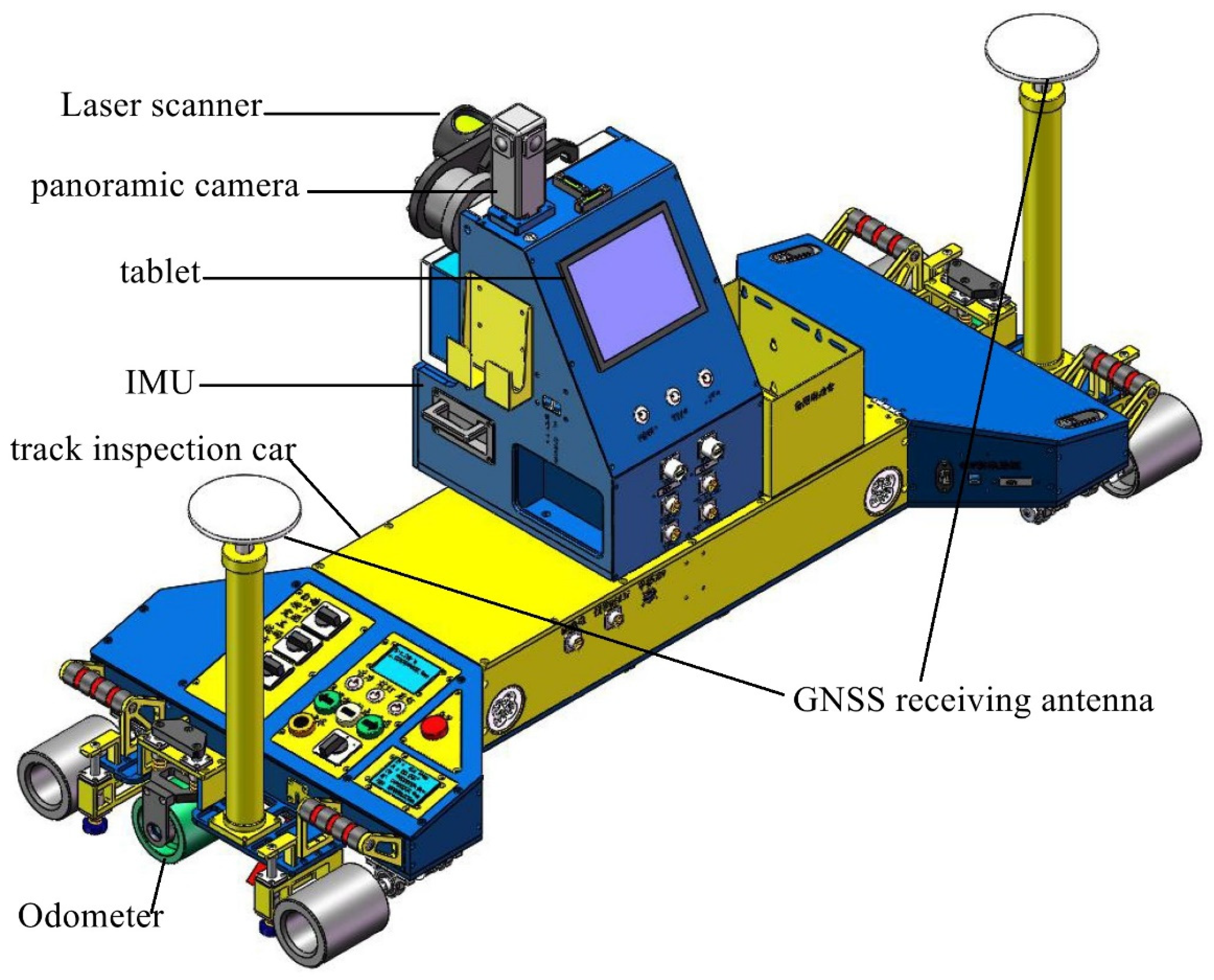
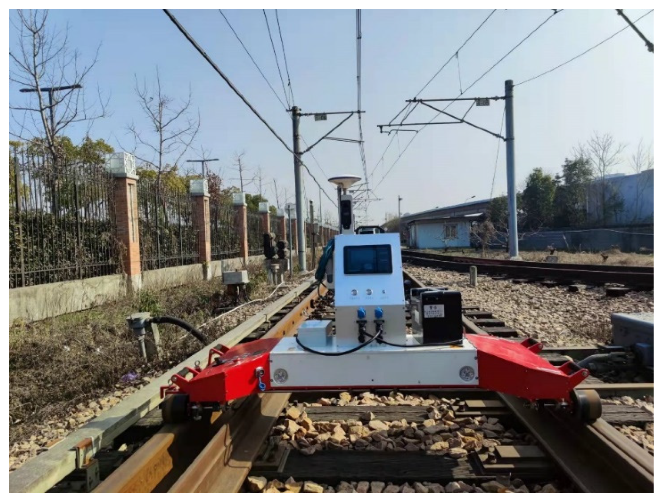
In order to achieve the purpose of three-dimensional absolute coordinate measurement, it is necessary to integrate the laser scanner and the position and attitude system into the system platform. Furthermore, the instrument platform is mounted on the mobile carrier to perform fast dynamic scanning during the carrier movement. Therefore, it is necessary to design a set of railway mobile laser scanning devices in-house. The self-developed system integrates two-dimensional cross-section laser scanners, INS, panoramic cameras, and a tablet into a mobile carrier that can run on the track.
Considering the ease of installation and disassembly of the platform, the occlusion of the camera’s field of view, the occlusion of the Global Navigation Satellite System (GNSS) antenna, and the stability of sensor installation, a multi-sensor integration box is designed. The platform integration design is shown in
Figure 1, which mainly includes: GNSS antennas, panoramic camera, laser scanner, tablet, and IMU. 10 mm aluminum alloy plates splice the main structure, and each plate has a weight reduction design. The outside is bent and welded by stainless steel plates to reduce exposed screws. The raw materials of each component must meet the requirements of lightweight and high rigidity. The data of scanner, INS, panoramic camera, and mileage are collected through a tablet, which adopts a capacitive touch screen and embedded wall-mounted installation. The present invention completes the startup of the device, the expansion of the power supply, and the transmission and downloading of data through the control panel, thereby simplifying the data transmission process. In the present invention, the scanner is fixed in the instrument case through the threads on both sides, which is convenient for installation and disassembly. A threaded interface is designed on the base of the instrument, which is suitable for various rail cars and official vehicles. The platform reserves total station and prism installation interfaces, and corresponding workbenches can be added according to subsequent needs.
The laser scanner selected in this paper is the German Z+F 9012 section scanner, which adopts the principle of laser ranging, emits laser pulses to the target surface, and records information such as distance, angle, and reflection intensity. To achieve fast and high-density acquisition of a large number of point cloud data of objects, the scanning rate of the system exceeds 1 million points per second, the maximum scanning speed is 200 rpm, and the distance resolution is 0.1 mm.
The inertial navigation system used in this article is the XD300A-DGI, which consists of a cost-effective closed-loop fiber optic gyroscope, an accelerometer, and a high-end GNSS receiving board. The bias stability of the inertial accelerometer is 5 × 10⁻⁵ g, and the bias stability of the gyro is 0.02°/h. The IMU consists of three accelerometers and three fiber optic gyroscopes. It is responsible for measuring the acceleration and angular velocity of the carrier and sending this information to the information processing circuit. The information processing circuit utilizes the acceleration and angular velocity measured by the inertial measurement unit for navigation and settlement. At the same time, using the satellite navigation information received by the GNSS board as a reference, comprehensive navigation is performed to correct the navigation error of the inertial navigation.
3. Methodology
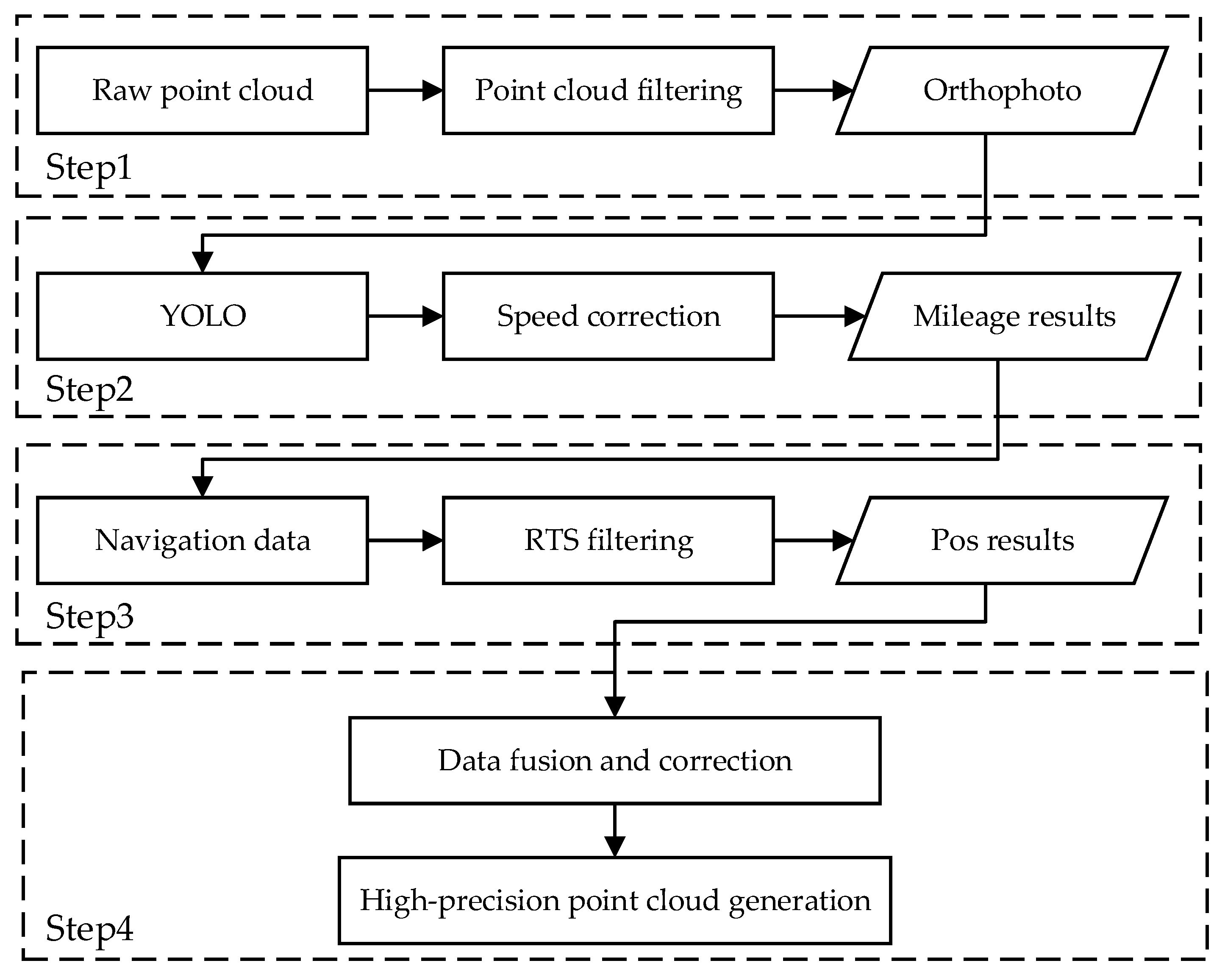
This paper divides the process of target detection and trajectory filtering into four steps: orthophoto generation, mileage localization method based on You Only Look Once (YOLO), location update and RTS trajectory filtering, and high-precision 3D point cloud reconstruction. The calculation flow chart is shown in
Figure 2.
3.1. Orthophoto Generation
The laser sensor emits a laser beam with a specific transmission power, and the laser beam is reflected and scattered when it reaches the surface of the object and is received by the laser sensor [
24]. The received echo power is obtained after processing by the internal system. The receiver converts the received power into voltage and digitally outputs an integer value, which is the intensity value. According to the scan lines, raster grayscale images are generated by performing projection expansion. The intensity value of the Z+F 9012 series laser scanner is stored in a 16-bit data length, and the acquired point cloud intensity range can be exported as [0, 1] or [0, 65,525] and other different grayscale ranges.
In order to highlight the difference in the point cloud intensity values of railway scanning feature objects, it is necessary to enhance the acquired point cloud intensity values. The full-scale grayscale histogram stretching method is adopted. The original intensity range is mapped to [0, 1] through a linear change. Let Q be the laser point set, and the original intensity value of each point is
W(
i),
i ∈ Q. Get the min and max in the raw intensity as follows:
Linearly map it to 0 and 255, respectively, to get the stretched strength value
:
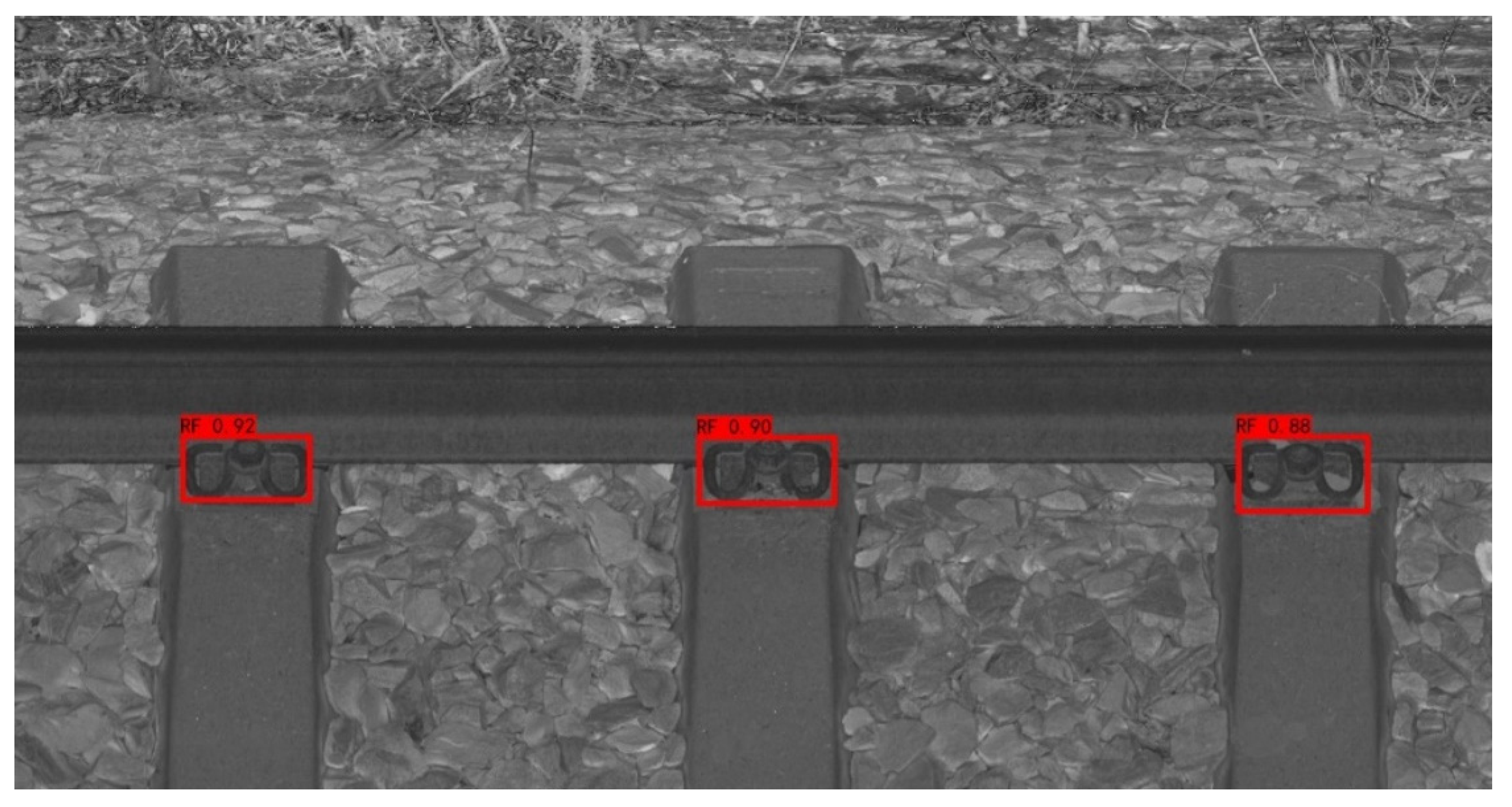
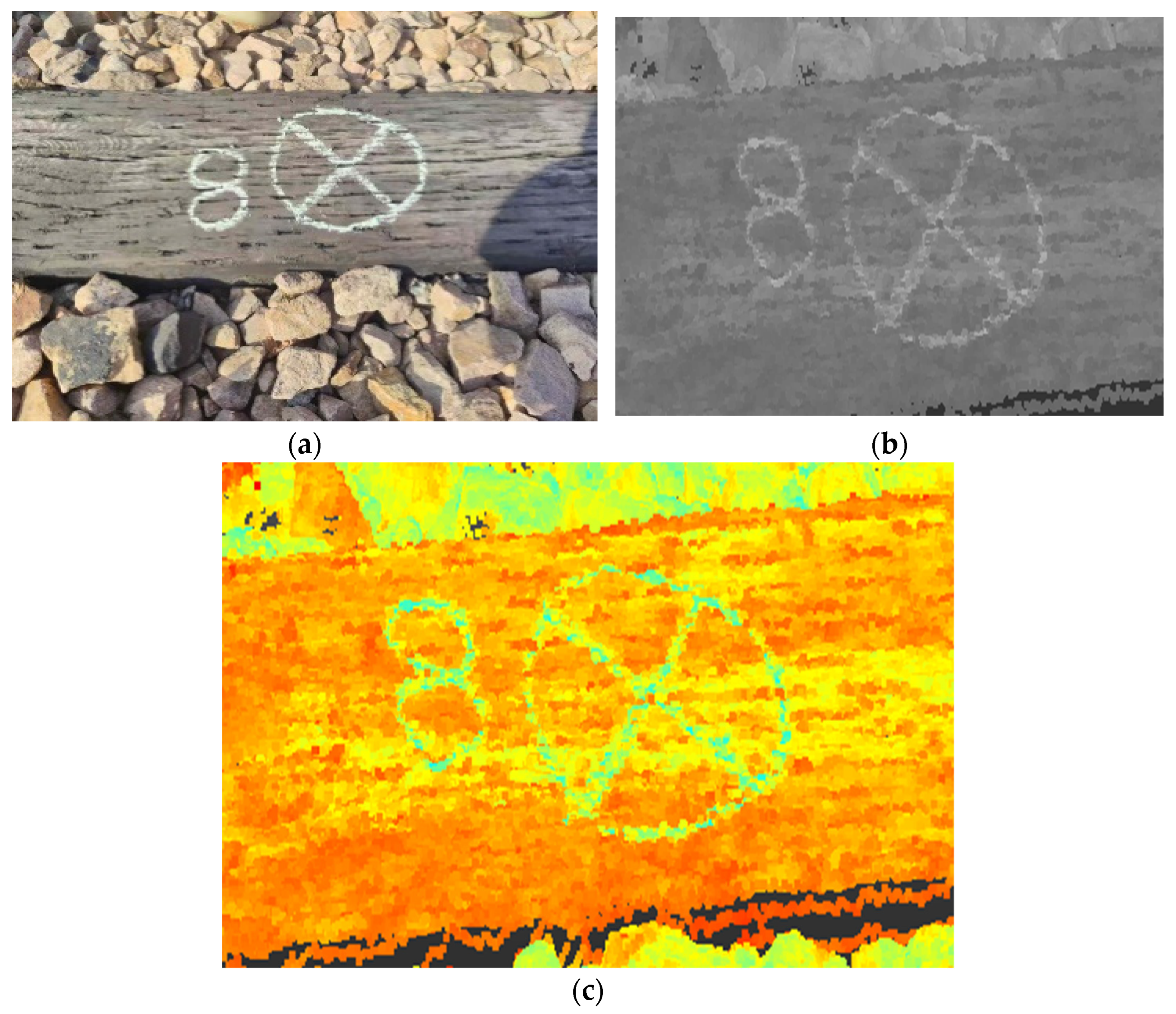
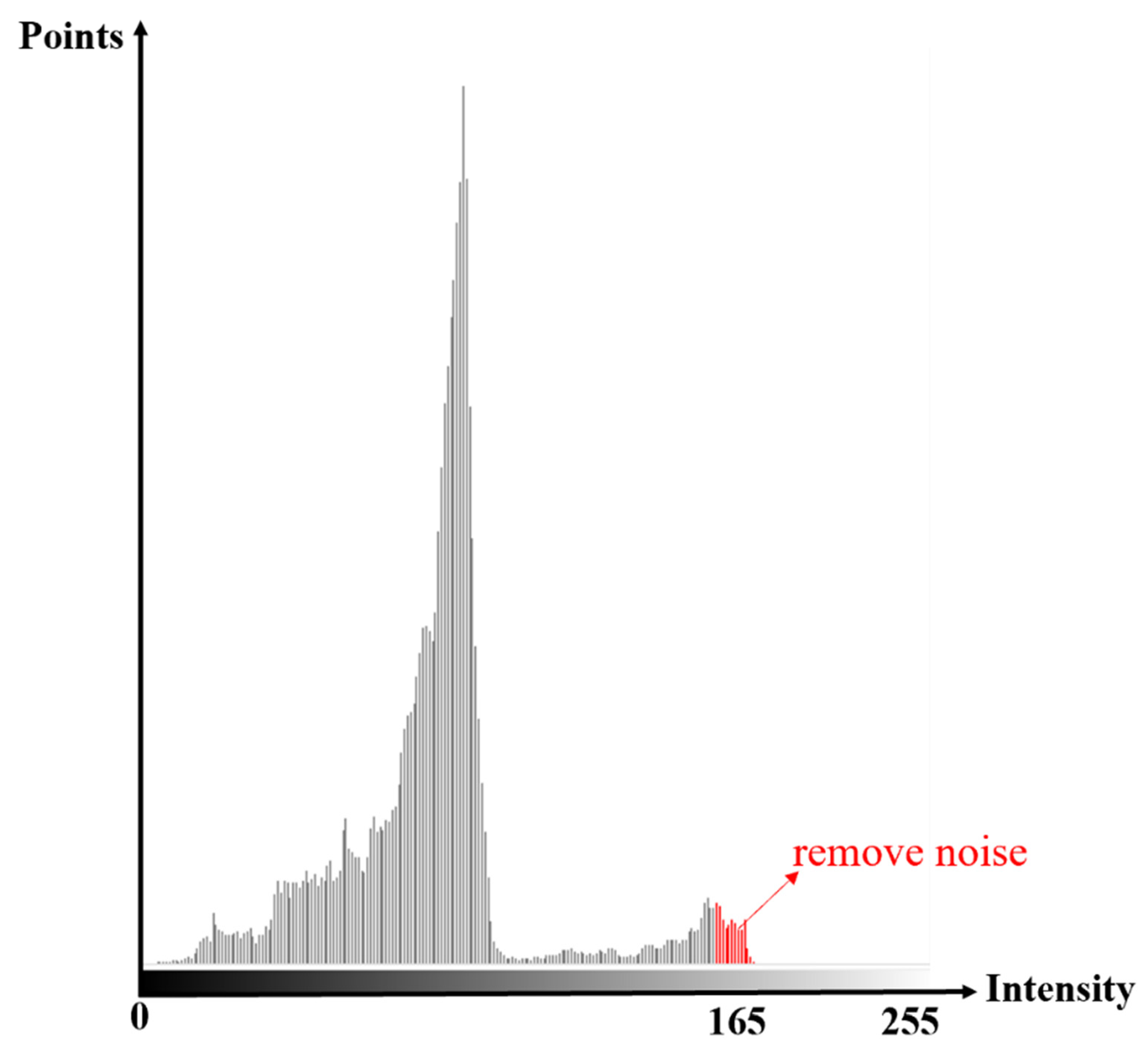
The original scanned point cloud has a small number of intensity minimum or maximum points. Only using this method to stretch the point cloud intensity value has certain defects. In order to solve this defect, on the basis of stretching the full-level grayscale histogram, an intensity value stretching method considering the number of point clouds is adopted. The minimum number of point clouds is used as a threshold to reduce the influence of intensity noise points. As a result, the intensity of the point cloud is firstly counted, the number of point clouds corresponding to each intensity value in the intensity value is obtained, and the histogram curve is drawn. As shown in
Figure 3, the minimum and maximum strengths with points greater than the threshold are counted as the minimum and maximum strengths of strength stretching. The intensity image is shown in
Figure 4.
A depth image, also known as a range image, refers to an image that uses the distance from the image collector to each point in the scene as a pixel value. The laser scanning system realizes the calculation of the depth image by comparing the time delay or phase of the transmitted signal and the received signal.
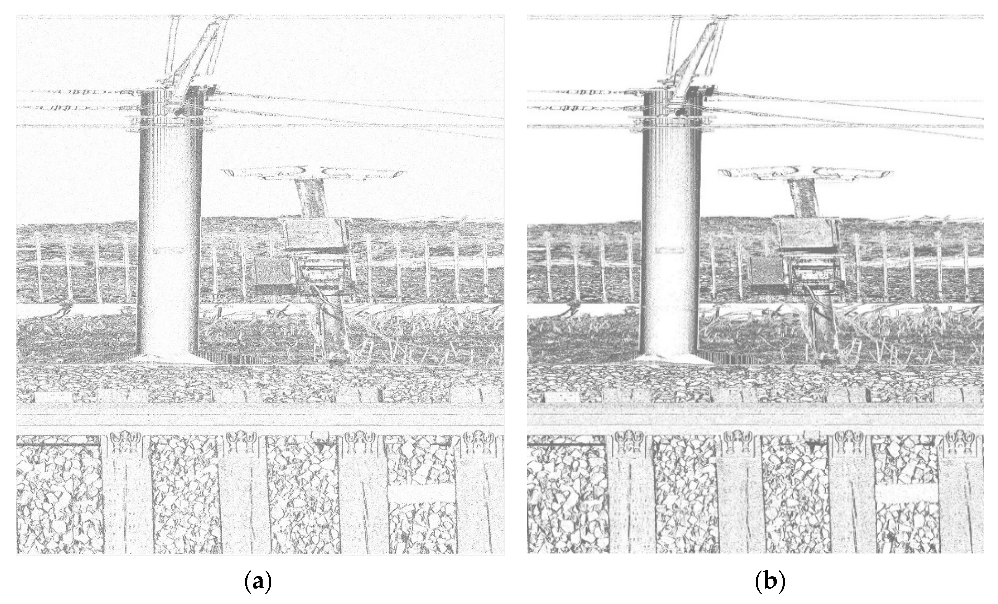
Firstly, the discrete laser point cloud data are resampled by the regular grid to obtain a digital depth (distance) matrix. Resampling is a method to determine the pixel value for any unknown point based on the four adjacent known pixel points. The pixel value of the unknown point is obtained by a first-order linear calculation in the horizontal and vertical directions. Different depth values are grayscale quantized and stretched. Taking this as the pixel value, we get a depth image that only contains the distance information. In this imaging process, interpolation errors are generated during resampling. For fewer errors, adaptive filtering of the resulting depth image is required.
Adaptive filtering is the process of dividing an image into sub-blocks and detecting the noise by applying it to the pixels in each sub-block. After adaptive filtering, the noise in the original image is suppressed, the main features of the image become more obvious, and the depth image is shown in
Figure 5.
The point cloud intensity filtering eliminates the influence of some external factors on the intensity value so that the point cloud intensity value is only related to the target reflectivity, which can improve detection accuracy. On the other hand, the distribution range characteristics of point cloud laser intensity values have been clarified by scanning various objects. The processing of point cloud depth images is mainly to enhance the expression of characteristic structures through image processing. Adaptive filtered images are used for target classification and identification based on geometric and spatial features of the structure.
3.2. Mileage Correction
3.2.1. YOLO Target Detection
At present, the method of mileage value acquisition is mainly based on an odometer. But the accuracy of the odometer is easily affected by complex environments such as wheel slippage, detection speed, and rail wear, resulting in cumulative errors in measurement results [
25]. In this study, the deep learning YOLOv3 target detection algorithm is used to extract regular feature points such as fasteners in the orthophoto. The method of equal-spaced correction is used to reduce the cumulative error effect caused by abnormal mileage values.
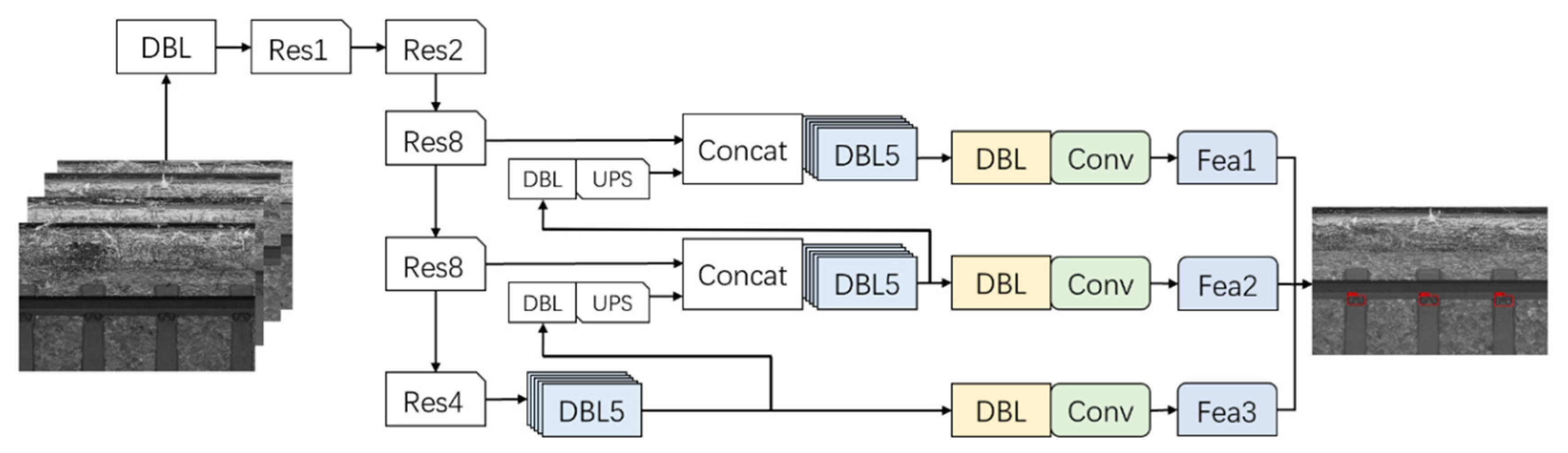
As one of the representative detection networks in the field of object detection, the YOLOv3 model is widely used in the field of rapid detection of small objects. YOLOv3 is a target detection algorithm with both accuracy and speed. It inherits and integrates the network structure of other target detection algorithms so that its overall performance has reached a high level. Its network structure is shown in
Figure 6 [
26,
27,
28]. As YOLOv4, YOLOv5, and others, have also been proposed one after another, it has been proved that the YOLO algorithm still has great potential for improvement [
29,
30].
Since the track fasteners to be identified are small object targets, the input of the network is modified from 416 × 416 × 3 to 533 × 533 × 3, and the resolution improvement is beneficial to retain more useful information. The multi-scale fusion operation of the feature pyramid is realized through multiple convolutions and up-sampling functions between the scale feature maps.YOLOv3 not only deepens the network depth through a large number of residual structures but also uses various methods such as feature fusion, multi-scale prediction, and bounding box regression to achieve a great improvement in detection speed and accuracy.
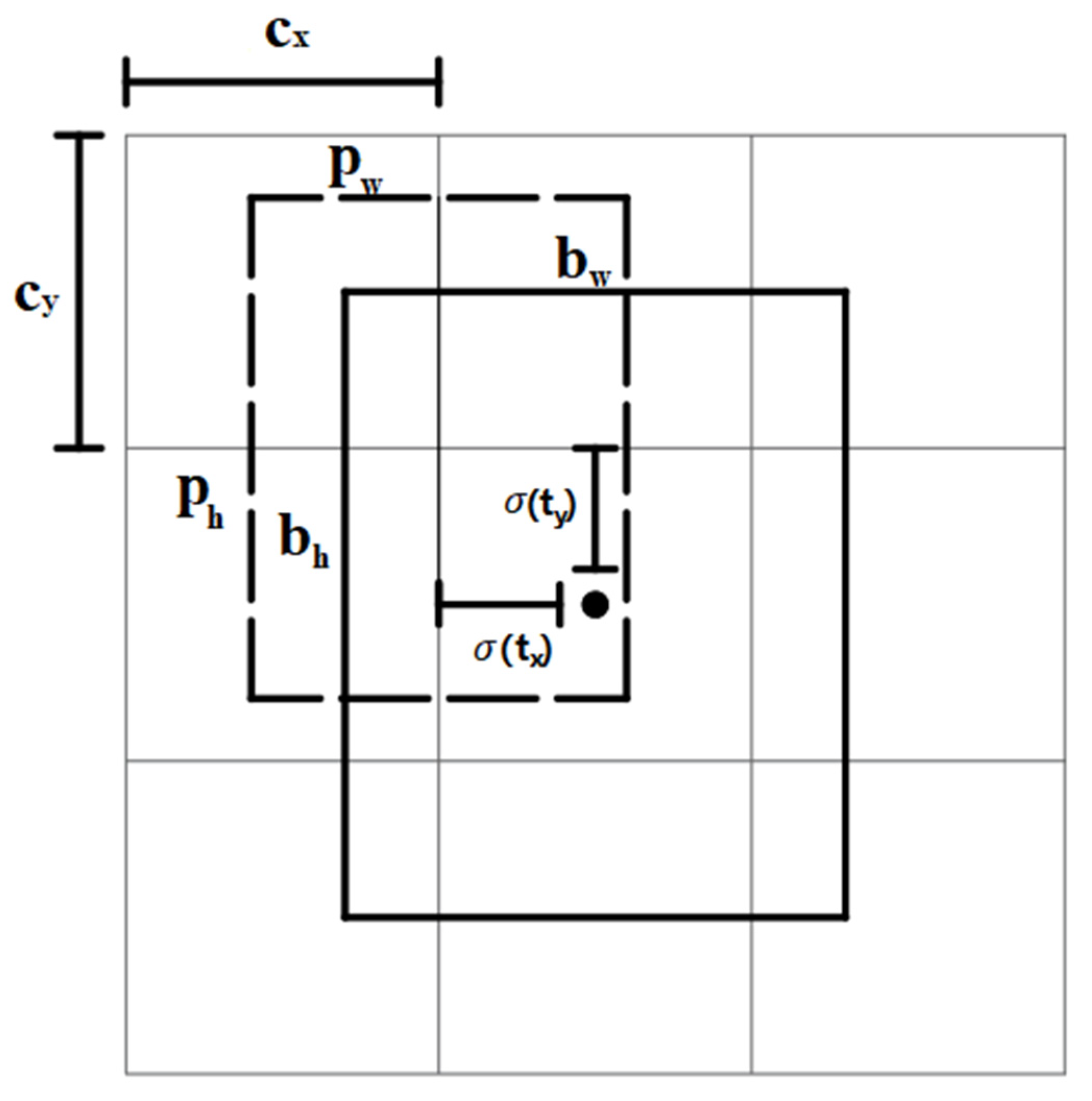
The relationship between the YOLOv3 target box and the prior box is shown in
Figure 7. YOLOv3 does not directly predict the position and size of the target but obtains the offset of the grid cell of the feature map by regression to determine the target’s center position. The size of the target is determined according to the scale factor of the target box size relative to the prior box.
The regression formula is:
In the formula, represents the center coordinates of the preset bounding box on the feature map; represents the width and height of the prior box on the feature map; represents the offset of the prediction center relative to the grid point; represents the predicted bounding box width and height scaling ratio; represents the final predicted target bounding box; σ represents the use of an activation function to scale the prediction offset into the interval 0 to 1.
In order to improve the speed of model training, the K-means method is used to perform cluster analysis of the data set, and the initial prediction frame parameters that are closer to the detection target in the orthophoto image are obtained. During the training process, in order to prevent overfitting caused by too many iterations, a loss value protection function is added to improve the stability of model training.
3.2.2. Performance Evaluation Indicators
The loss function is an important indicator for evaluating the model’s performance. During the model’s training process, the parameters in the network are continuously adjusted, and the value of the loss function loss is optimized to minimize the model’s value to complete the model’s training. The loss function of YOLOv3 consists of three parts, including confidence loss (
), class loss error (
) and localization loss (
),
are balance weight coefficients. The loss function can be specifically expressed by the following formula:
The target confidence loss (
) is expressed as:
In the formula, represents the confidence score, and oi represents the ratio of the predicted box to the ground-truth box.
The target class loss (
) is expressed as:
In the formula, Oij represents the binary cross-entropy loss, and Pij represents the probability of the existence of the j-th object in the predicted object bounding box.
The target localization loss is expressed as:
In the formula, represents the value of the coordinate offset processed by the activation function, and represents the coordinate offset between the real frame and the default frame.
The algorithm test in this paper uses Mean Average Precision (
), Recall, and Precision to evaluate the performance of the algorithm. The evaluation formulas are:
In the formula,
AP represents the accuracy rate corresponding to each target, and
m represents the total number of target object categories.
In the formula, TP is the positive detection rate, that is, the calibration is a positive sample, and the actual detection is also a positive sample; FP is the false detection rate, that is, the calibration is a negative sample, and the actual detection is a positive sample. FN is the missed detection rate; it is calibrated as a positive sample, and the actual detection is a negative sample.
The target detection system filters out useless target boxes below the threshold according to the settings of the confidence threshold and the intersect over the union threshold. If the threshold is too high, it may cause some real targets to be filtered out and missed. If the threshold is set too low, some targets for model error detection will not be filtered out and will be treated as normal targets. This paper selects the best confidence threshold through multiple tests. When the confidence threshold is 0.50, and the intersect over union threshold is 0.55, more targets are correctly detected, and no false targets occur. Finally, we use the above thresholds for model training to ensure that more correct targets are detected.
3.2.3. Mileage Constraints and Positioning
Due to the complex environment of mobile scanning, the YOLO target detection algorithm has certain errors, and only deep learning cannot extract all the coordinate information of feature points. Therefore, this paper first adopts the method of distance clustering to segment the target set of fasteners identified by deep learning. If the number of targets in the clustering set is less than three, the set is not calculated. This method can effectively eliminate the feature information that is wrongly identified and count the number of missing feature points. Secondly, the missing fastener feature points are complemented using Lagrangian interpolation, and their coordinate values can be expressed as:
In the formula, t is the missing feature node; p0, p1, p2, ..., pn are the feature points obtained by clustering. y0, y1, y2, ..., yn are the abscissa values in the pixel coordinate system corresponding to the cluster feature points.
According to the obtained abscissa information of the feature points and the starting and ending mileage information of the measurement interval, the accurate mileage value corresponding to each feature point can be obtained, which solves the problem that the image coordinates do not match the actual mileage in the mobile measurement. The main calculation process is as follows:
(1) Mileage constraint: Calculate the total length D of the interval according to the information of the starting and ending mileage plates. According to the target detection result, the pixel interval
of the feature point is obtained. Combined with the change value y of the abscissa of the start and end pixels, the interval value
of each feature point is calculated. We obtain the mileage value between the feature points according to the pixel value interpolation method:
In the formula, represents the length of the known start and end points, and represents the mileage value of the feature points identified by target detection. represents the pixel interval between start and end points, represents the pixel interval of consecutive feature points.
(2) Initial positioning: Starting from the initial feature point mileage, iteratively accumulate the interval values of each feature point to obtain the mileage value of each feature point. According to the position of the pixel in the pixel interval
, we obtain the mileage value of the pixel point
:
In the formula, represents the initial mileage of any pixels, and represents the pixel values within adjacent feature points.
(3) Speed analysis: According to the scanning frequency f of the laser scanner, the time interval
of the scanning line is calculated. The corresponding speed
is obtained based on the finite element method, and the mean filtering method is used to further optimize the speed value. The influence of the noise in the system on the speed value is weakened, and the speed value
of the moving carrier in each period is obtained.
In the formula, represents the mean filter, and represents the window size of mean filtering. represents the time interval between adjacent scan lines, represents the initial velocity value, and represents the filtered velocity value.
(4) Mileage correction: Correct the initial mileage value according to the optimized speed value to obtain the final mileage value
.
In the formula, represents the mileage value of adjacent pixels after filtering, and represents the mileage value of the target point after filtering.
3.3. Inertial Navigation Data Processing Model
3.3.1. Location Update Algorithm
Dead reckoning is a technology that uses the known position, combined with the moving speed and bearing, to estimate the existing position [
31]. Because it does not need to receive external signals, it is suitable for estimating the position of the mobile measurement system in the position without a GNSS signal. Furthermore, we can form an inertial navigation system with the data of the GNSS navigation data to overcome the shortcoming that the accumulated error will increase with time.
When the inertial navigation data are used as the original data for position update, the attitude update adopts the quaternion algorithm, and the formula is as follows:
In the formula, are real numbers, are both mutually orthogonal unit vectors and imaginary units .
The projection of the carrier measured by the accelerometer relative to the inertial frame into the local coordinate system, namely:
In the formula, represents the specific force output of the accelerometer, and represents the specific force projected to the local coordinate system. and represent the pose matrices of two adjacent moments, respectively.
Using rectangular integration for the velocity differential equation gives:
In the formula, represents the velocity of the motion carrier obtained in the current epoch, represents the velocity of the motion carrier in the previous epoch, Δt represents the epoch interval, is an obliquely symmetric matrix formed by the angular velocity of the carrier rotating relative to the local geographic coordinate system, and represents the local gravity vector at the location of the carrier.
It is easy to derive from the position differential equation:
Usually using trapezoidal integration to solve the above equation, we get:
In the formula, and represent the position of the motion carrier at adjacent times.
For the case of fusion calculation of odometer and inertial navigation data, it is necessary to use vehicle non-integrity constraints to assist in the calculation. For the convenience of research, the odometer measurement coordinate system is established, the y-axis is in the ground plane in contact with the carrier wheels and points to the front of the vehicle body, the z-axis is perpendicular to the ground plane and is positive, and the x-axis points to the right. Assuming that the carrier trolley does not drift, derail, and shake up and down when the vehicle runs as normal on the railway, the sky and lateral velocities can be set to 0 as constraints. According to the above definition, the speed output of the odometer in the navigation coordinate system can be obtained:
In the formula, represents the forward speed of the odometer, represents the speed vector of the odometer in the odometer coordinate system, and represents the speed vector of the odometer in the navigation coordinate system.
The components of the odometer in the east, north, and sky directions of the navigation system are:
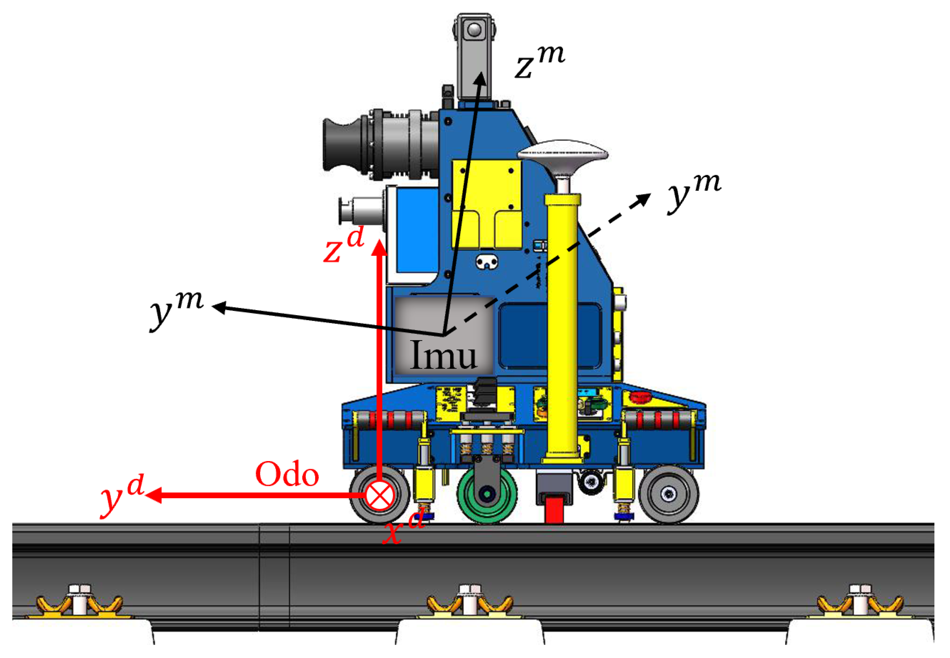
3.3.2. Installation Declination Error
In the inertial navigation system, the velocity measured by the odometer is usually projected to the inertial navigation coordinate system. In practical applications, the odometer coordinate system and the inertial navigation coordinate system often do not coincide, and an installation error needs to be calibrated and compensated, as shown in
Figure 8.
Assuming that the transformation matrix between the odometer coordinate system and the inertial navigation coordinate system is
,
represent the pitch angle, roll angle, and heading angle of the odometer coordinate system relative to the inertial navigation coordinate system. The attitude matrix is:
In the case that the three installation error angles are all small angles, the above attitude matrix can be simplified as follows:
Let
, then:
In the formula, I is the identity matrix; φ× represents the cross-product antisymmetric matrix constructed by each component of φ.
The projection of
on the inertial navigation coordinate system is:
The speed of the vehicle in the navigation system can be obtained from the inertial navigation system output and the attitude transformation matrix is obtained from the inertial navigation output. Taking the quantity on the left side of the equal sign in the formula as the measured value and φ as the estimated value, the corresponding state can be estimated by the recursive least squares method.
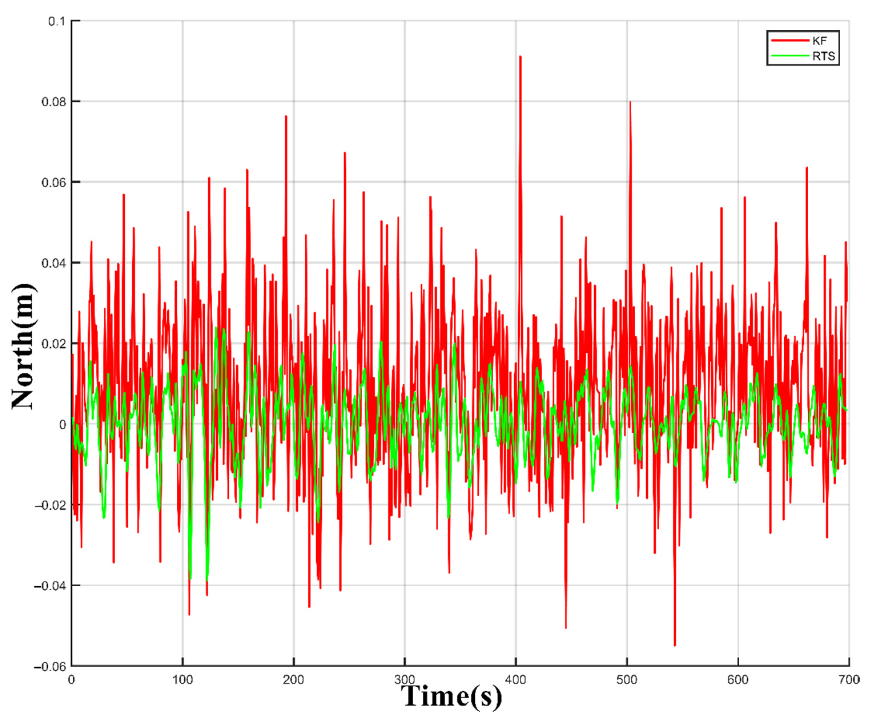
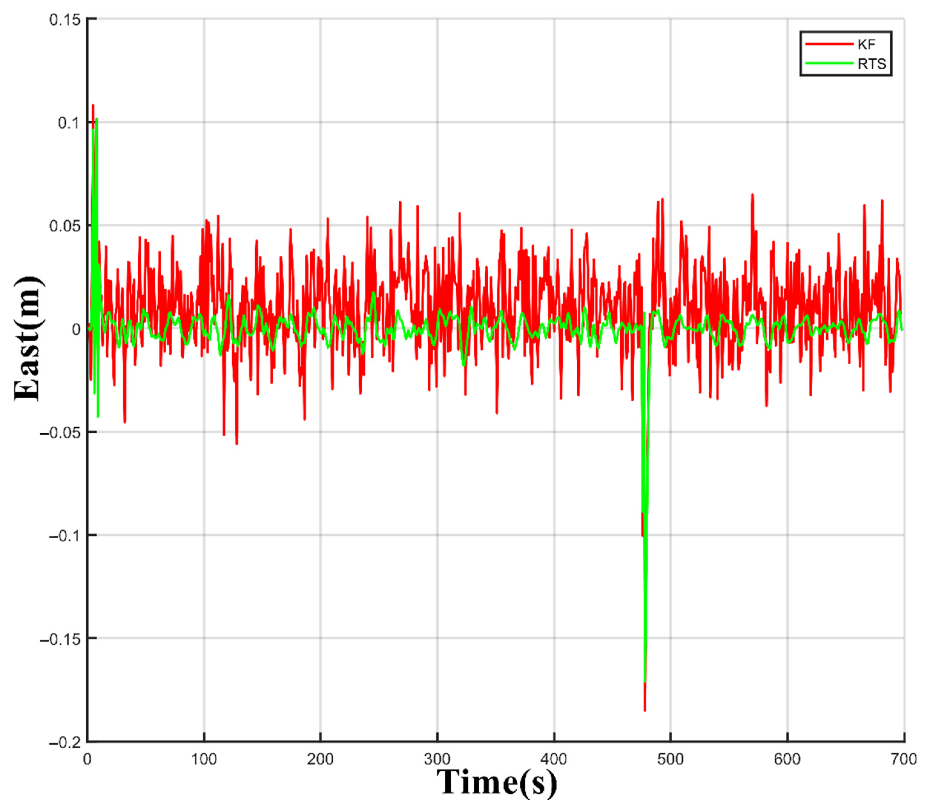
3.3.3. RTS Filtering
A Kalman filter is an estimation method. Kalman filtering can estimate parameters in the system in real-time, such as continuously changing position and velocity, among others. The estimator is updated with a series of noise-contaminated observations, which must be a function of the parameter to be estimated, but may not contain enough information to determine a unique estimate over a given time.
After obtaining adequate information, the Kalman filter uses prior knowledge, such as deterministic and statistical properties of system parameters, as well as observations to obtain the optimal estimate, which is a Bayesian estimate. On the basis of the provided initial estimates, the Kalman filter performs a weighted average of the prior values and the new values obtained from the latest observation data through recursive operations to obtain the latest state estimates [
32]. In order to achieve the optimal weighting of data, the Kalman filter has estimation uncertainty and can give the correlation measure between estimation errors of different parameters. This is achieved with step-by-step iterations of parameter estimation, which also incorporates the uncertainty of observations due to noise.
Since the 3D point cloud generation based on multi-sensor fusion uses the original data to estimate the trajectory position error as the observation update of the Kalman filter, when there is an observation update, the error of the position estimation and its covariance is tiny. However, due to the existence of residual systematic errors, the position measurement estimation error and its covariance between two observation updates will gradually increase with time. In order to obtain a high-accuracy position estimate in the whole measurement process, it is necessary to make full use of all observations to update the constraint error through an appropriate algorithm, which is a typically fixed interval smoothing problem. In the fixed interval smoothing algorithm, the commonly used methods mainly include the forward and backward Kalman filter smoothing algorithm and the RTS smoothing algorithm. The two algorithms are equivalent in theory, and the RTS smoothing algorithm is relatively simple to implement. In this paper, the RTS smoothing algorithm is used to process the data in the orbit measurement interval [
33,
34,
35].
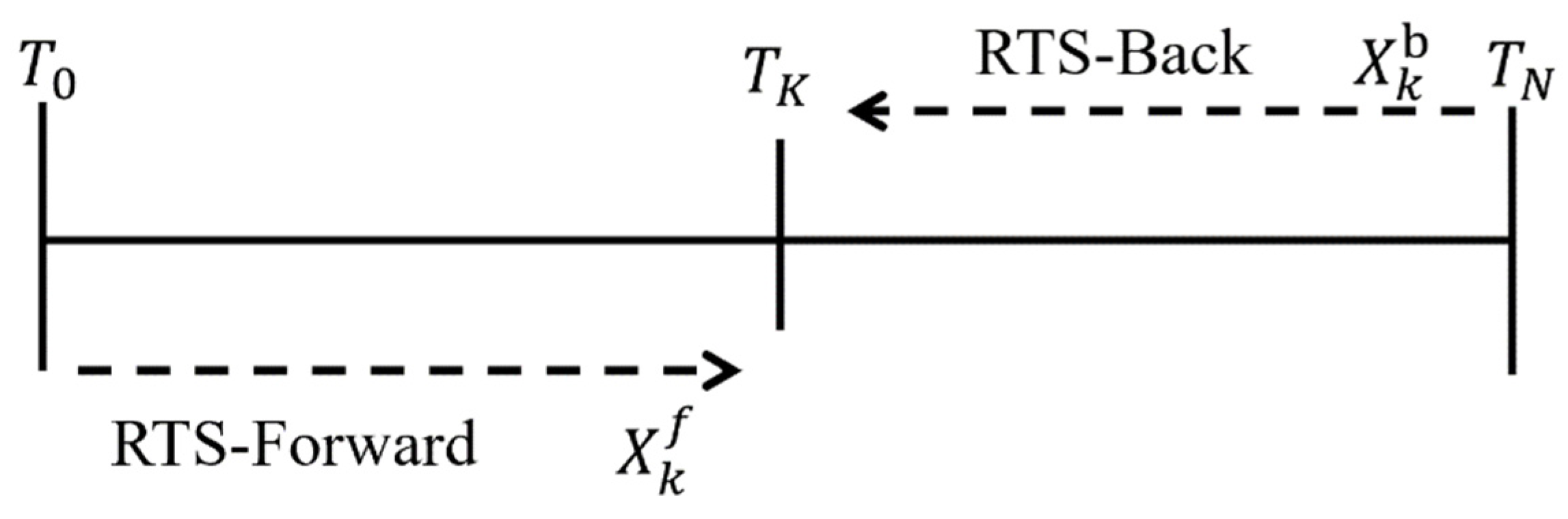
The RTS smoother consists of a typical forward Kalman filter and a reverse smoother. After each system propagation and observation update, the system state vector, error covariance matrix, and state transition matrix are recorded. After the data reaches the end, the data is smoothed from the endpoint to the start point in the reverse direction. The calculation flow of the RTS smoothing algorithm is shown in
Figure 9:
The forward filtering of the RTS smoothing algorithm is a typical Kalman filter, and the smooth estimated value of the state vector is a weighted combination of two filtering estimated values. The calculation process is as follows:
In the formula, and represent the optimal filter estimation value and its covariance matrix of the forward filtering state vector at time t, and represents the optimal one-step predicted value of the state vector and its covariance matrix at time t of the forward filtering, is the observation matrix at time t, and is the optimal gain matrix of the forward filtering at time t. represents the system state transition matrix, which can be obtained from the system error matrix , and is the discrete noise matrix at time t of the forward filter.
The inverse smoothing process can be expressed as:
In the formula, and are the optimal smoothing estimation value and its error covariance matrix of the RTS smoothing algorithm at time t. is the optimal smoothing gain matrix of the RTS smoother at time t.
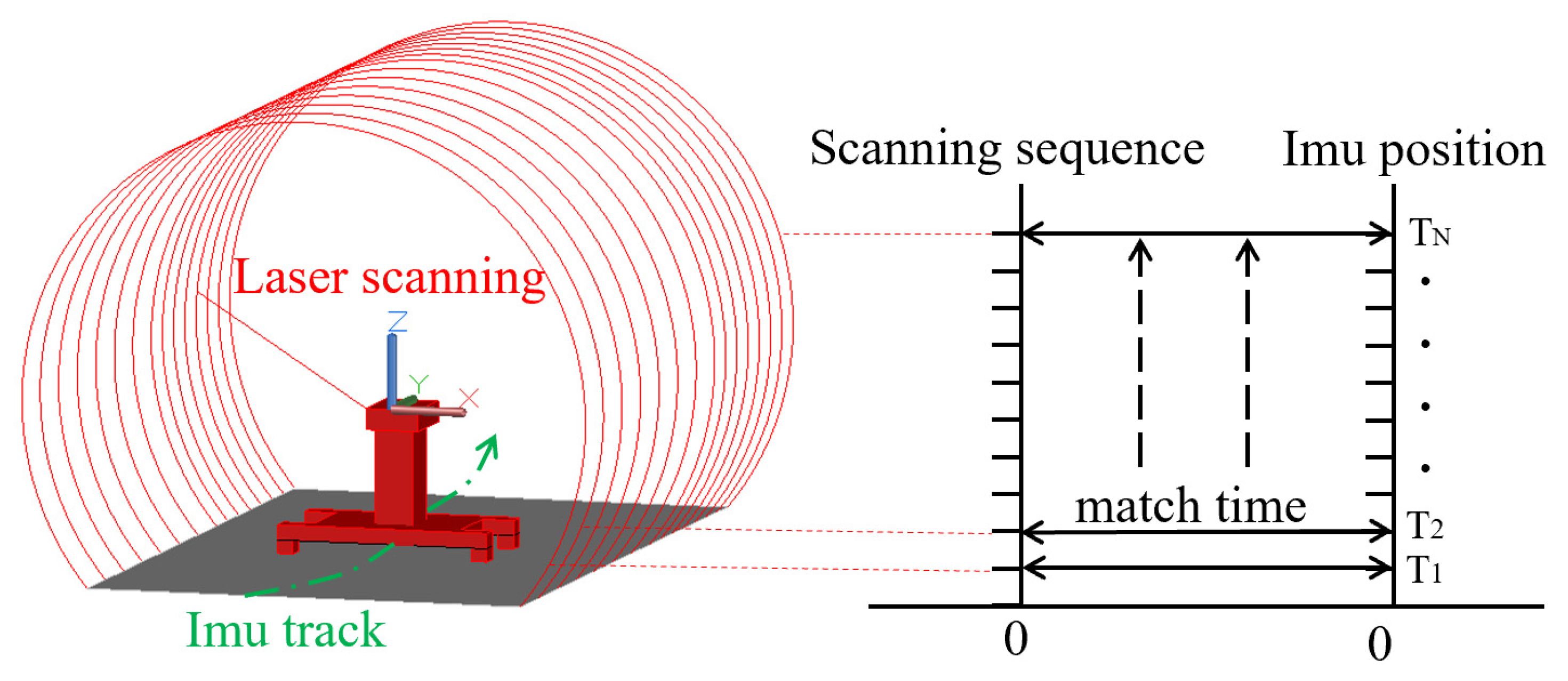
3.4. High-Precision Point Cloud Generation
One of the keys to multi-source data fusion of mobile scanning systems is time registration. First, the field data acquisition achieves zero-time identity through the synchronous control of integrated acquisition software. In the post-processing process, the data matching of the adjacent moments is carried out through the phase time interval to realize the consistency of the data, as shown in
Figure 10.
After the time synchronization between the sensors is completed, the relevant sensor data under the same time reference can be obtained, and the spatial calibration of the system hardware can unify the relevant sensor data on the same spatial reference. According to the transformation relationship between the coordinate systems and the model parameters, the scan data can be converted from the scanner coordinate system to the vehicle body coordinate system by using the calibration parameters of the system. Combined with the position and attitude data of the vehicle body coordinate system with the GNSS antenna phase center as the origin of the coordinate system calculated by the INS, the scanned data can be converted from the vehicle body coordinate system to the data in the absolute coordinate system. Finally, the 3D point cloud data based on the absolute coordinate system is obtained by completing the fusion processing of multi-source data.
The point cloud calculation formula for converting the point cloud data from the scanner coordinate system to the absolute coordinate system is:
In the formula, is the section coordinates based on the scanner coordinate system after the original Z+F 9012 scan data is parsed; the original data is recorded by the inertial navigation system. Combined with the body trajectory position parameters , the rotation matrix is provided by the combination of three attitude angles (yaw, pitch, roll); The translation matrix and rotation matrix are obtained from the system calibration obtained from the scanner coordinate system to the vehicle body coordinate system.
Through the above calculation formula, the original data obtained by the scanner can be used to post-process the data of the inertial navigation system, combined with the transformation principle of the coordinate system, and finally, the 3D point cloud data based on the absolute coordinate system can be obtained.
5. Discussion
In this study, the deep learning method is used to extract the track feature points, the Lagrange interpolation is used to complete the missing feature points, and the speed filtering method is used to optimize the mileage in segments. In an interval of 20 meters, the mileage accuracy is controlled within 1 decimeter so as to reduce the influence of the cumulative error caused by the odometer as much as possible. In the traditional method, it is necessary to reduce the influence of the cumulative error caused by the slippage of the odometer by increasing the fixing device between the trolley and the track. Still, this method will gradually increase the error over time and reduce the work efficiency. At present, the target detection algorithm used in this paper is YOLOv3, and more advanced target detection algorithms such as YOLOv7 can be used in the future to obtain better recognition accuracy and speed of track feature points.
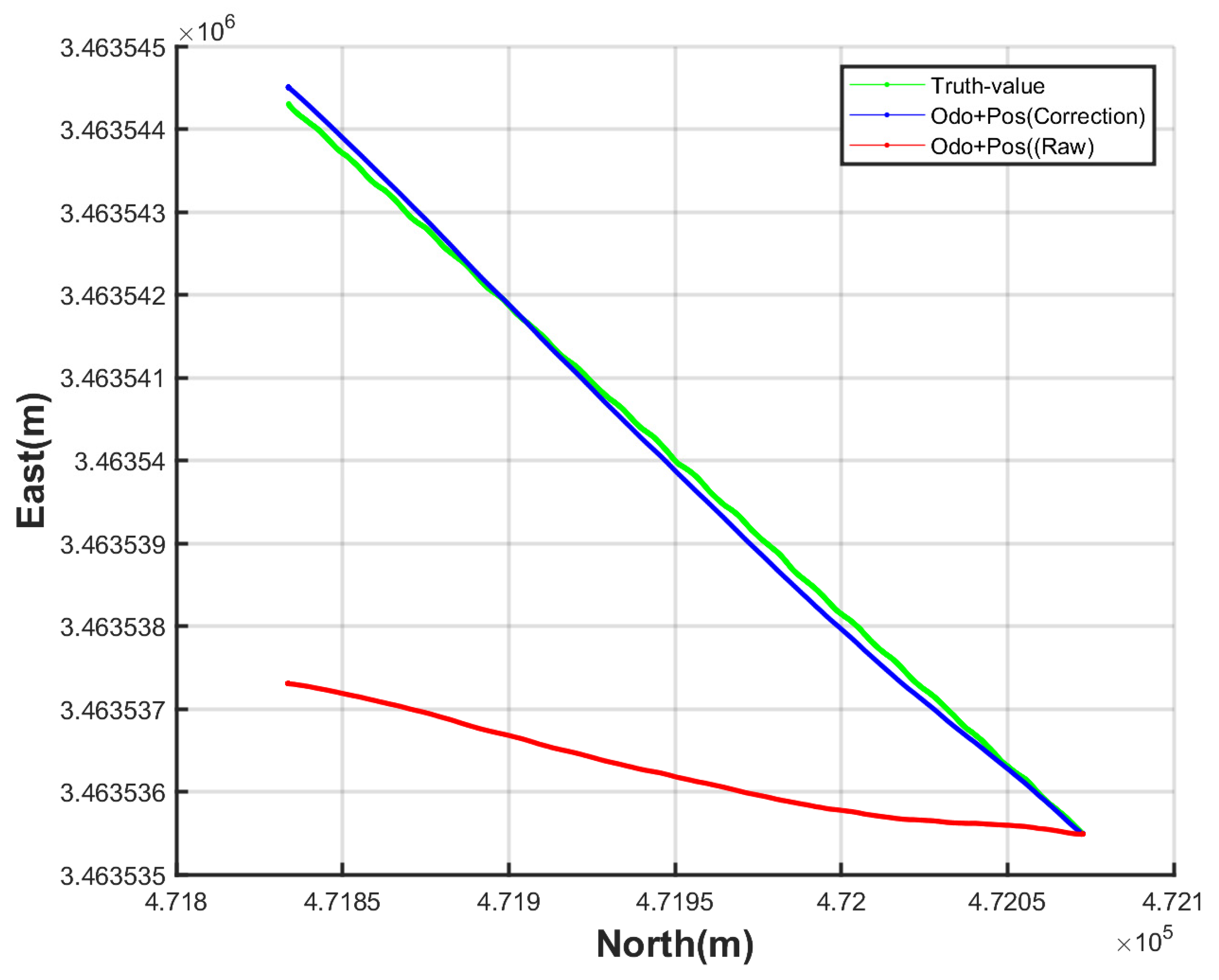
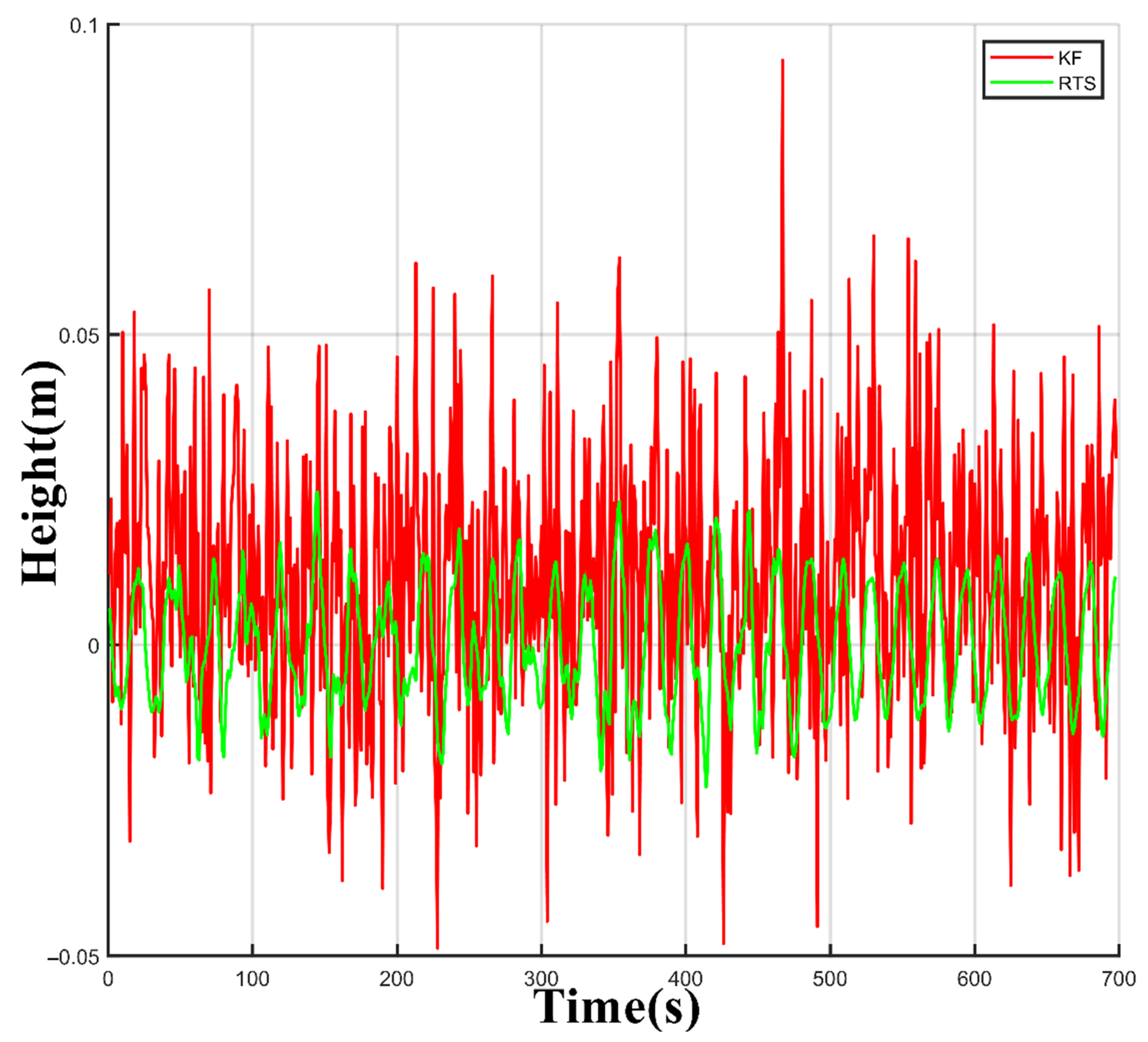
In this paper, the RTS smoothing algorithm is used to smooth the dead reckoning results, and the experiments show that smoothing has a great effect on improving the accuracy of post-processing. Due to the complex and changeable railway environment, the GNSS signal is often blocked. At this time, it is necessary to use an appropriate method to compensate for the drift of the inertial navigation system. In addition to the smoothing algorithm proposed in this paper, the commonly used method of dynamic zero-speed correction can only slow down the drift speed of the error but cannot completely limit the drift of the error. Therefore, in order to obtain better trajectory results in the subterranean environment, it is necessary to use higher-precision IMU in the future and continue to study and optimize the proposed IMU trajectory error model to improve the practicability of the system.
In the future, we will add visual sensors and simultaneous localization and mapping (SLAM) algorithms to optimize the trajectory to adapt to complex railway environments such as mountain tunnels. At the same time, the conversion relationship between the measurement coordinates and point cloud coordinates based on the control points is studied, and the trajectory data is further corrected by segmental fitting to obtain a higher-precision railway three-dimensional point cloud.
6. Conclusions
In this study, we adopt a mileage correction algorithm based on visual feature points and use deep learning to detect objects in the generated orthophoto. Then, RTS filtering is used to optimize the dead reckoning trajectory, and the real motion trajectory of the mobile carrier is restored. The multi-source data fusion method is used to obtain the railway point cloud data in the absolute coordinate system.
The experimental results show that the mileage correction method has good positioning accuracy and stability, and the mileage positioning error is within about 6 cm, which provides accurate mileage results for trajectory calculation. The 3D point cloud data is generated by combining the trajectory generated by the RTS filtering algorithm and the scanning data. The maximum errors of the 23 coordinate points measured are all within 7 cm. The average error of the point position is 1.60 cm, and the average error of the elevation is 2.39 cm.
Different from the traditional method that uses manual detection of railways, this paper proposes a new method using the combination of calibrated mileage and inertial navigation data. The mileage is calibrated segmentally using visual feature points, which avoids multiple stops of the mobile laser scanning system for calibration. It reduces the influence of the trajectory error increasing with time in the traditional method. There is no relevant research on this method yet.
The measurement method combined with laser scanning and inertial navigation can quickly obtain the real 3D scene point cloud in the absolute coordinate system. The speed and amount of information at the measuring point far exceed traditional methods. In the future, according to the point cloud data, we can complete the extraction of railway elements, including the track centerline, contact wire, and catenary wire. Moreover, 3D models of railway buildings can be built from point cloud data. At the same time, high-precision point cloud data can help us to complete the information of infrastructure along the route quickly. It is of great significance in railway digital survey and design, intelligent operation and maintenance, and digital transformation.


