Article

Assessing the Impact of Neighborhood Size on Temporal Convolutional Networks for Modeling Land Cover Change

by
Alysha van Duynhoven
* and
Suzana Dragićević
Spatial Analysis and Modeling Laboratory, Department of Geography, Simon Fraser University, 8888 University Drive, Burnaby, BC V5A1S6, Canada
*
Author to whom correspondence should be addressed.
Remote Sens. 2022, 14(19), 4957; https://doi.org/10.3390/rs14194957
Submission received: 15 July 2022 / Revised: 28 September 2022 / Accepted: 30 September 2022 / Published: 4 October 2022
(This article belongs to the Special Issue Machine Learning Techniques Applied to Geosciences and Remote Sensing)

Abstract

:
Land cover change (LCC) studies are increasingly using deep learning (DL) modeling techniques. Past studies have leveraged temporal or spatiotemporal sequences of historical LC data to forecast changes with DL models. However, these studies do not adequately assess the association between neighborhood size and DL model capability to forecast LCCs, where neighborhood size refers to the spatial extent captured by each data sample. The objectives of this research study were to: (1) evaluate the effect of neighborhood size on the capacity of DL models to forecast LCCs, specifically Temporal Convolutional Networks (TCN) and Convolutional Neural Networks (CNN-TCN), and (2) assess the effect of auxiliary spatial variables on model capacity to forecast LCCs. First, each model type and neighborhood setting configuration was assessed using data derived from multitemporal MODIS LC for the Regional District of Bulkley-Nechako, Canada, comparing subareas exhibiting different amounts of LCCs with trends obtained for the full region. Next, outcomes were compared with three other study regions. The modeling results were evaluated with three-map comparison measures, where the real-world LC for the next timestep, the real-world LC for the previous timestep, and the forecasted LC for the next year were used to calculate correctly transitioned areas. Across all regions explored, it was observed that increasing neighborhood sizes improved the DL model’s capabilities to forecast short-term LCCs. CNN–TCN models forecasted the most correct LCCs for several regions while reducing error due to quantity when provided additional spatial variables. This study contributes to the systematic exploration of neighborhood sizes on selected spatiotemporal DL techniques for geographic applications.

1. Introduction

Land cover changes (LCCs) arise from human activities and environmental processes that alter the condition of the Earth’s surface [1], contributing directly and indirectly to environmental changes in regional and global systems [2]. The interconnection of LC with local, regional, and global systems makes studying and forecasting LCCs a vital component in fields such as geography [3] and climatology [4]. The proliferation of open LC datasets has resulted in the increasing use of computational approaches such as deep learning (DL) methods for classification and modeling tasks [5]. Neural networks of expanding breadth and depth underpin DL algorithms, facilitating complex pattern recognition in remote sensing data sources [6]. To forecast LC given a remotely sensed image timeseries, temporal DL models called Recurrent Neural Networks (RNNs) and Temporal Convolutional Networks (TCNs) can be used to obtain patterns from sequences.
Many research studies use timeseries data extracted from each cell or pixel comprising historical raster GIS data layers to classify LC and to forecast LCCs presuming enough data is available [7,8]. For example, TCNs were used to project vegetation cover with multitemporal remotely sensed data [8]. However, these research studies extracted temporal sequences from each cell comprising the raster data layers, excluding consideration of proximal LC dynamics. While temporal sequences provide historical information of individual cells comprising a raster, influences occurring within the neighborhood of each cell are also important for LCC modeling [9]. In order to extract spatial features from a neighborhood in DL models, Convolutional Neural Networks (CNNs) are typically used to process neighborhoods provided as a grid of cells at each timestep before extracting temporal patterns [5]. Models containing CNN and temporal DL techniques are often referred to as “spatiotemporal” models and have been leveraged in past studies on land change applications. For example, a model composed of LSTM layers is considered a temporal model. Therefore, CNN and LSTM layers can be integrated to implement spatiotemporal models, such as CNN–LSTM.
Constructing a dataset from a multi-temporal geographic data source for spatiotemporal DL models requires a neighborhood to be specified. Previous research studies have used a variety of neighborhood settings for land change modeling and classification. For instance, land change classification and forecasting applications involving datasets with spatial resolutions of 30 meters used Moore neighborhoods spanning 3 × 3, 5 × 5, and 9 × 9 cells [10,11,12]. With finer spatial resolution training data samples, 9 × 9 neighborhoods were specified to classify LC with DL models [13]. With coarser spatial resolution data, 11 × 11 neighborhoods and below were found to better capture nearby land change interactions [14]. Neighborhood dimensions not following the Moore neighborhood convention also involved 10 × 10 [15], 32 × 32 [5], and 64 × 64 neighborhood settings [16] with 10 and 20 meter spatial resolution datasets. However, despite the range of neighborhood dimensions investigated in previous studies, the impact of neighborhood dimensions on DL models for the task of LCC forecasting is undetermined. While it is acknowledged that neighborhoods encompassing hundreds or thousands of pixels from fine spatial resolution data are commonly used in other applications such as change detection, the relationship between neighborhood size and a model’s capacity to forecast LCCs is unknown.
Only a few studies have explored the influence of neighborhood sizes on the outcomes of DL methods used for LC classification and modeling and were primarily selected for reasons such as to operate within computational constraints [16], to maintain available dataset qualities or formats [5], or to optimize overall accuracy measures [12]. They may also be specified arbitrarily [11,17]. It becomes difficult to determine optimal neighborhood settings from the current literature for the task of modeling LCC with DL. Thus, further systematic exploration of the relationship between neighborhood size and capacity of DL models to forecast LCCs is needed. Additionally, TCN and CNN–TCN models are unexplored with neighborhood settings beyond cell-level sequences for LCC forecasting or with other spatial drivers of LCC. Therefore, the main objectives this research study were to: (1) evaluate the effect of neighborhood size on the capacity of DL models to forecast LCCs, specifically TCN and CNN–TCN, and (2) assess the effect of auxiliary spatial variables on model capacity to forecast LCCs. Preliminary outcomes were explored with respect to datasets for the Regional District of Bulkley-Nechako in the province of British Columbia (BC), Canada, where trends were first explored for subareas and the entire region. Next, the findings obtained for the full region were compared with those obtained for three separate regions in the province. Lastly, the influence of spatial variables was compared across model and neighborhood configurations applied to all four regions. Experiments conducted on the respective datasets used two temporal DL models (LSTM and TCN) and two spatiotemporal models (CNN–LSTM and CNN–TCN). The purpose of using the LSTM and CNN–LSTM models was to provide a baseline for comparing the TCN and CNN–TCN model performance, because they are more commonly used. Outcomes were examined using change-focused metrics. The specific details of the research work are outlined in the next sections.

2. Methodology

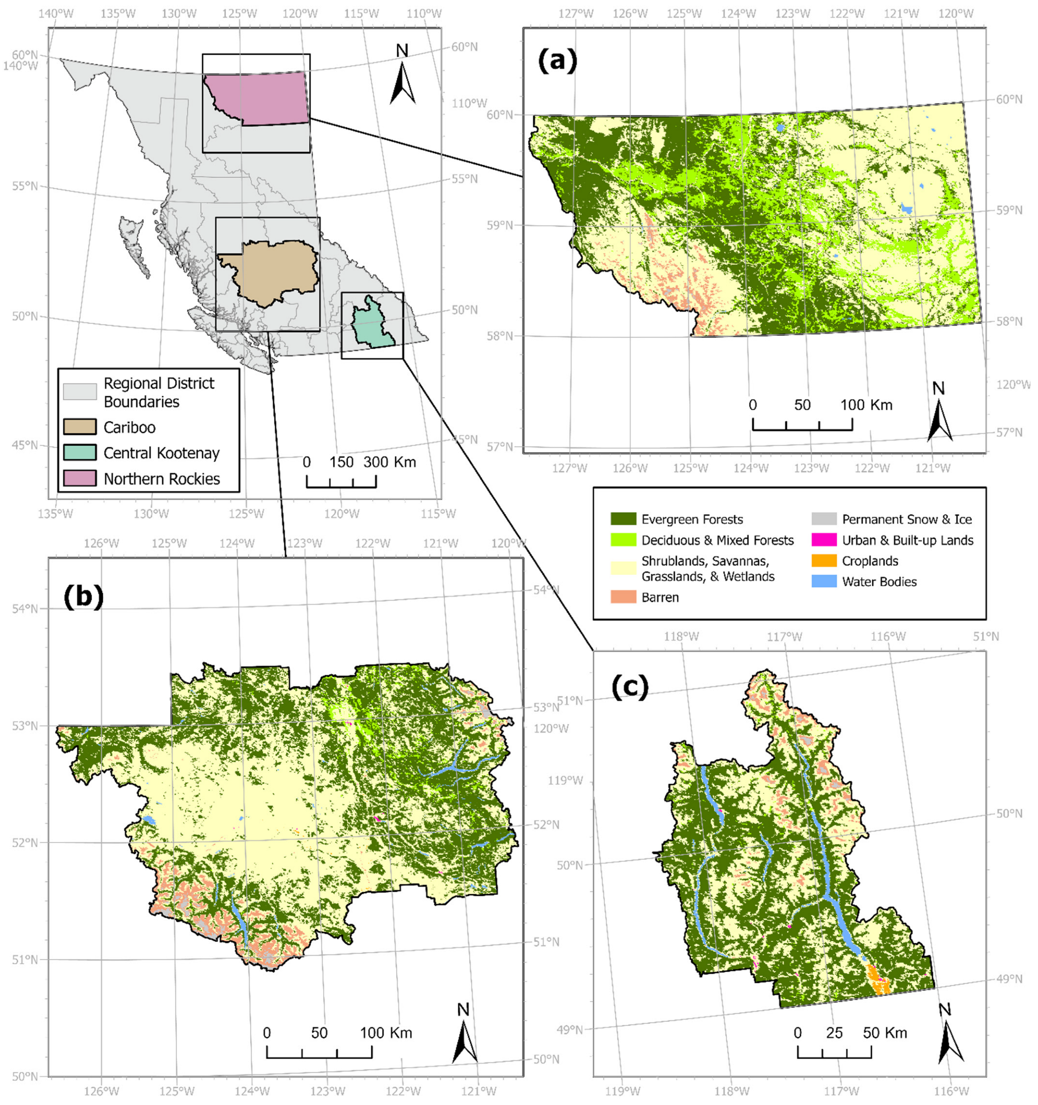
2.1. Study Area and Datasets

The primary experimental study area used was the Regional District of Bulkley-Nechako, located in northern BC (Figure 1). LCCs over the past two decades have been characterized by a notable loss of forested areas in this region (Table 1). The spatiotemporal LC dataset was obtained from the Terra and Aqua combined Moderate Resolution Imaging Spectroradiometer (MODIS) Land Cover Type (MCD12Q1) dataset [18] featuring yearly temporal resolution data from 2001 to 2019. The Land Cover Type 1: Annual International Geosphere–Biosphere Programme (IGBP) classification data layer featuring 17 LC classes was used for this study. In particular, the IGBP raster product was provided at a 0.05° spatial resolution, which is approximately 463.31 m spatial resolution in the Bulkley-Nechako region [19]. LC classes were aggregated based on previous research studies [20] to produce eight classes including: (a) evergreen forests, (b) deciduous and mixed forests, (c) shrublands, savannas, grasslands, and wetlands, (d) barren land, (e) permanent snow and ice, (f) urban and built-up lands, (g) croplands, and (h) water bodies. To support the exploration of trends across experiments, three alternative study areas were also considered (Figure 2). These include the Regional District of Central Kootenay, the Northern Rockies Regional Municipality, and the Cariboo Regional District, where the amount of change between 2001 and 2019 differs from the primary experimental study area (Table 1).
In addition to spatiotemporal LC data, seven static spatial variables were included to capture drivers of LCCs. The selected variables capture a single snapshot of factors related to accessibility and topography. Accessibility factors used in prior LCC applications and adopted in this research study include the proximity to various features, including proximity to population centers [21], roads [22], railways [23], lakes and rivers [24], and coastal waters [25]. These were derived by computing the Euclidean distance from each feature using the point and vector data layers available from Statistics Canada [26,27]. Topographic variables involved in prior LCC studies include elevation and slope [28]. The ASTER Global digital elevation model was used to source the elevation data and derive the slope data layer for this research study [29].
All datasets are reprojected to the NAD 1983 BC Environment Albers projected coordinate system where planar area measurements are preserved. Spatial data layers are resampled to or computed relative to the MODIS LC data, which has the coarsest spatial resolution. Bilinear interpolation was used to resample the DEM. Edge effects were minimized by eliminating the influence of cells outside of the study region, with a 2.78 km buffer from the edges of the study area [30].

2.2. Overview of Deep Learning Models

Four models were implemented in this research study, including two temporal DL models (LSTM and TCN) and two spatiotemporal models (CNN–LSTM and CNN–TCN). All models were implemented with Python 3.9.1 [31], the Keras API [32], and TensorFlow 2.5.0 [33]. The open-source KerasTCN API was used to implement the TCN and CNN–TCN models [34].

2.2.1. Temporal Models (LSTM and TCN)

LSTM models are extensively used to model temporal patterns [35]. The development of LSTM models occurred in response to the vanishing gradient problem that affected traditional RNN approaches for long timeseries data [36,37]. The unique features of an LSTM unit include “gating” functions and internal memory cells which maintain, drop, or inhibit the flow of information through an LSTM unit [38]. The main equations of an LSTM are expressed in previous studies [38]. The LSTM models specified in this research study feature two LSTM layers with 32 and 128 units, respectively, that use the default tanh activation function [11]. The layers are followed by a dropout regularization factor of 10% informed by previous studies [11,39]. Dropout regularization inhibits networks from overfitting by randomly dropping a specified percentage of neurons [40]. The fully-connected output layer features 9 neurons to forecast the likelihood of each of the 8 LC classes. The activation of the output layer is the Softmax function which is useful for multi-class forecasting and classification problems [41]. Neighborhood inputs are provided as one-dimensional arrays for each timestep, described in detail in Section 2.2.3.
TCNs are also used to obtain long-term patterns from sequential data [42]. While TCNs are used for extracting proximal temporal features, they also benefit from the highly parallelizable structure of CNNs, providing a less computationally intensive alternative to LSTM models. The primary components of a TCN model include a one-dimensional, fully convolutional network to extract temporal patterns and dilated causal convolutions, which prevent the purging of historical information [43]. Dilations enable the receptive field to expand exponentially, thus preserving longer-term information from sequential datasets. The formulation of TCNs has been discussed in detail in prior research studies [42]. The implemented TCN models are characterized by two layers featuring 32 and 128 filters, respectively, using the ReLU activation function. Filters characterizing a TCN refer to a vector of learnable weights. The dilations parameter setting is 1,2,4, and 8 [44], and the kernel size is set to 2 [45]. The kernel refers to a matrix of weights that is multiplied with each subset of the input sequence. To match the LSTM model implementation, a dropout factor of 10% is applied before the output layer featuring the Softmax activation function. Neighborhood inputs are provided as one-dimensional arrays for each timestep, described in Section 2.2.3.

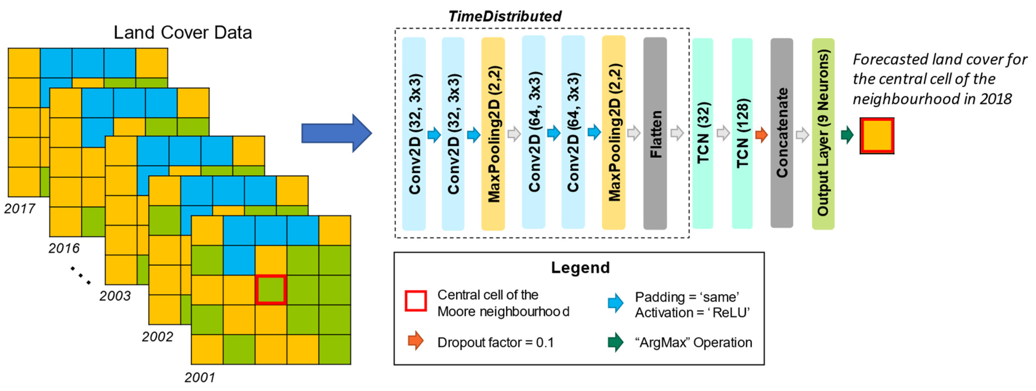
2.2.2. Spatiotemporal Models (CNN–LSTM and CNN–TCN)

In combinations of spatial and sequential DL techniques, spatial features are often first extracted using Convolutional Neural Networks (CNNs). CNNs can be used to obtain abstract spatial features from remotely sensed imagery [6]. The formulas describing CNNs have been disseminated in previous research studies [12]. Through a combination of convolutional layers and pooling layers, spatial patterns from a two-dimensional raster or image can be extracted [46]. This makes a CNN a useful construct for extending the spatial coverage of sequential DL models beyond per-cell timeseries to capture the states of neighboring cells [9]. As such, CNNs facilitate the extraction of spatial relationships present within a neighborhood at each timestep, while temporal relationships are captured using a sequential DL approach. Such models are commonly used for video recognition tasks (i.e., CNN–LSTM [47]) that require spatial dependencies to be first extracted before obtaining temporal dependencies from samples of independent videos. However, in geographic applications employing raster data layers, training datasets are populated by extracting spatiotemporal neighborhoods or “patches” across the study area, where the spatial coverage of each sample is specified by the neighborhood dimensions.
In this research study, CNN–LSTM and CNN–TCN were implemented to extract spatial relationships within neighborhoods of each cell for each timestep. These spatiotemporal DL models were implemented first with a single-branch input structure that accepts the LC data sequences only, adapted from prior model implementations [48,49]. LC sequences were provided as input to a branch consisting of four CNN layers and two 2 × 2 max-pooling operations (Figure 3). The CNN layers feature 32, 32, 64, and 64 filters, respectively, each followed with a ReLU activation function. Using multiple CNN layers and expanded filter sizes facilitates the extraction of increasingly complex spatial features [50]. The CNN layers were each parameterized with a 3 × 3 kernel, zero-padding, and a stride of one [11]. A 3 × 3 kernel size was specified given the sample input dimensions [51,52] and to obtain local relationships of LC from sample neighborhoods [53]. Likewise, while increasing kernel sizes may be beneficial for finer-scale spatial resolution data for the purpose of extracting larger scale features [54], the coarser spatial resolution of the data and sample input dimensions used in this research study are better suited to a smaller kernel size for considering the local context of LC. The CNN operations were followed by a dropout factor of 10%. The TimeDistributed functionality afforded by the Keras API enables these operations to be applied to each timestep in the sequence of LC data provided [11]. This facilitates the extraction of spatial features from each timestep. Outputs of this branch were flattened, then provided as inputs to the sequential layers. For example, TCN layers are shown in Figure 3 following the concatenation operation. In the CNN–LSTM approach, this was replaced with LSTM layers with 32 and 128 units, respectively. The general structure of the CNN–TCN model is inspired by a previous approach demonstrating how outputted feature vectors from CNNs were provided as inputs to TCNs for a video classification task [55]. However, the CNN–TCN model structure in this research study does not require the advanced CNN component for the MODIS LC data. The CNN–TCN model was implemented with TensorFlow and KerasTCN, with TCN layers parameterized the same as in Section 2.2.1.

2.2.3. Neighborhood Effects in Deep Learning Models

For each cell, the influence of neighborhood composition and changes within it are referred to as the “neighborhood effect” [56]. In this research study, DL models were used to obtain the strength of neighborhood effects and influential spatiotemporal patterns from samples without user intervention. The spatial coverage of neighborhood effects is controlled by specifying a neighborhood size, which is a highly influential parameter in land change modeling endeavors [56,57,58]. It should be noted that the term “neighborhood” is synonymous to spatiotemporal data “tiles” (i.e., [5]) or “patches” (i.e., [17,52]) prepared for DL model training datasets described in some research studies. The terms “tiles” or “patches” were previously used to refer to some M × M area obtained from an overall study region, where M refers to the number of cells along the longest edge of the cell neighborhood. This research study follows the Moore neighborhood convention, where a target cell refers to the cell located at the center of the neighborhood. For example, a 3 × 3 Moore neighborhood contains a target central cell and the eight surrounding cells [58]. Moore neighborhoods contain N cells given a distance range parameter r, where N = ( 2 r + 1 ) 2 . The neighborhood sizes explored in this study and their respective surface areas they cover given the spatial resolution of the dataset are presented in Table 2. The neighborhood dimensions selected to explore with the DL models are based on previous findings that showed that including cells 2.5 km to 3.5 km from the central cell captured the characteristics of neighborhoods with 500 m spatial resolution data [14].
In this research study, the task of LCC forecasting was framed as a spatiotemporal DL problem with respect to the CNN–LSTM and CNN–TCN modeling techniques. The intended effect of including neighborhoods in DL models is to capture a range of influence surrounding each cell by integrating information about state changes occurring near a central cell. For CNN–LSTM and CNN–TCN models, neighborhoods surrounding each target cell at each timestep are provided explicitly as the model’s input. For example, these models accept spatiotemporal inputs in the form of T × M × M × C, where T denotes the number of timesteps, M denotes the neighborhood dimension, and C denotes the number of LC classes. For the temporal models, LSTM and TCN, the neighborhood structure is not inherently preserved. In previous studies, the states of each neighboring cell were explicitly provided as variables to LSTM models in the form of a one-dimensional array for each timestep [11,17]. To provide neighborhoods of size 3 × 3 and larger to the temporal models, the process of “flattening” neighborhood information to compatible one-dimensional sequences was carried out. This means that the T × M × M × C spatiotemporal input sequence for each cell was transformed to a one-dimensional array with dimensions T × M × M × C, where M × M × C is the length of the input vector at each timestep.

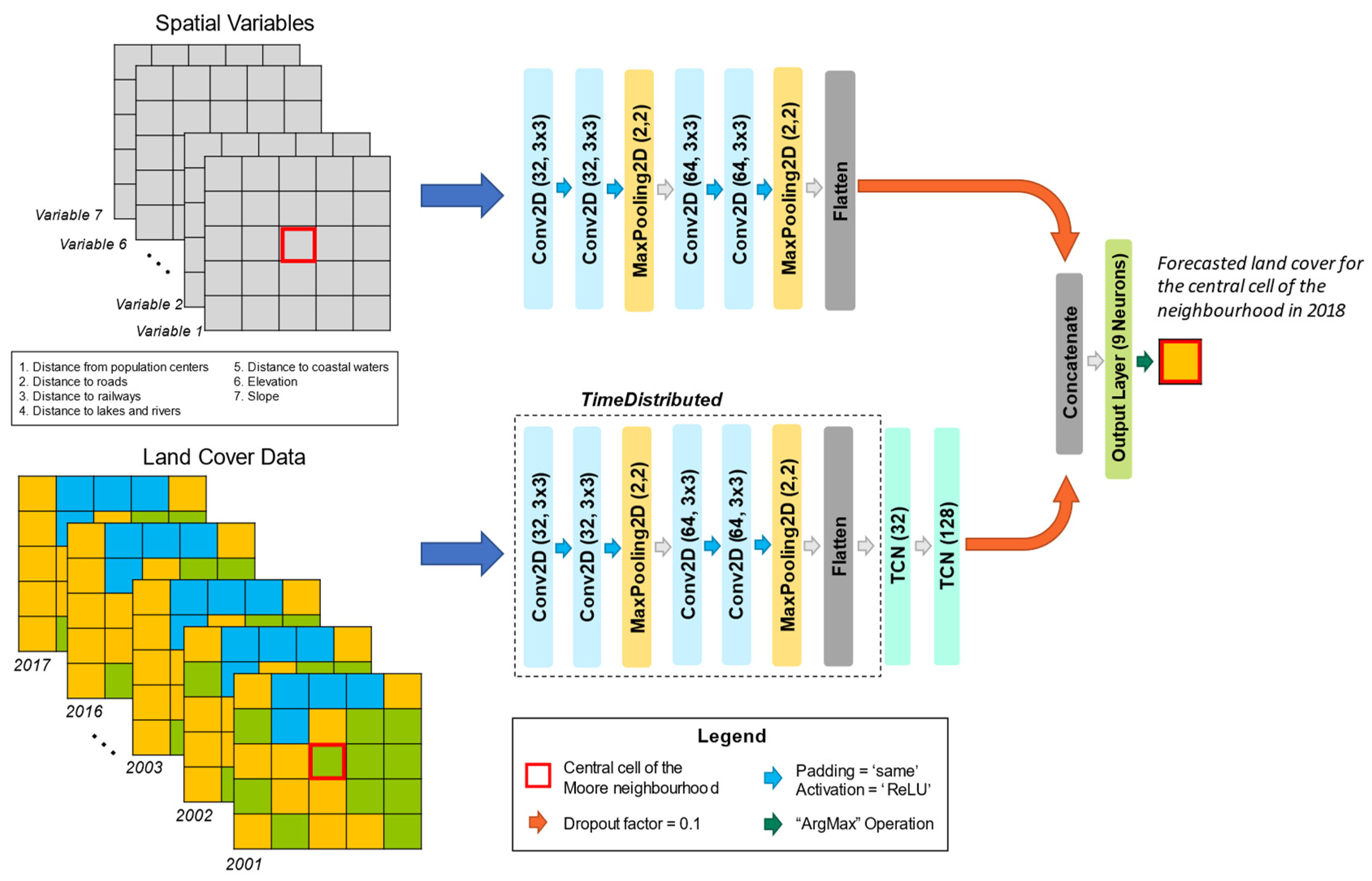
2.2.4. Adding Spatial Variables

To accommodate both spatiotemporal LC data and static spatial variables, the previous single-branch model was extended for the spatial variable input (Figure 4). This structure was expanded from previous studies [48,49]. For the multi-branch model implementation used to add the spatial variables for the Case 3 experiments, the LC input branch implementation is the same. The second branch of the model uses convolutional layers to extract spatial relationships from the seven spatial variables of each training sample. Six convolution layers, 2 × 2 max-pooling operations, and dropout regularization were used to process the auxiliary spatial features (Figure 4). The number of filters parameterizing each CNN layer of this branch was 32, 32, 64, and 64, respectively. Outputs of the spatial input branch were flattened and combined with outputs from the LC data branch using the concatenation operation. The activation function of all CNN layers is ReLU and the output layer with 9 neurons uses the Softmax function.

2.3. Overview of Experiments

The LSTM, TCN, CNN–LSTM, and CNN–TCN models were explored in three experimental cases. Real-world multi-temporal MODIS LC data and static spatial variables were used to forecast one year of LCCs for the selected study regions. LSTM and CNN–LSTM models were used as a baseline to compare TCN and CNN–TCN models, as the former are more common in geographic applications. Case 1 considered the LC data of the Regional District of Bulkley-Nechako (R1) to explore whether trends in the model’s capacity to forecast LCCs for three subareas is similar to that observed for the full region from which they were extracted from (Figure 1). Next, Case 2 explored the respective models on separate study regions, including the Regional District of Central Kootenay (R2), the Northern Rockies Regional Municipality (R3), and the Cariboo Regional District (R4) (Figure 2). Outcomes from Case 1 and the additional regions were compared to identify recurring trends. Lastly, Case 3 explored the effect of the spatial variables branch across model types and neighborhood sizes.
The temporal resolution of the models was one year. A “rolling-window” forecasting scheme used a specified interval to train the model, while the interval is advanced by one year to test the model by evaluating its capacity to project the next timestep [59]. The LCC modeling task was framed as a multi-class forecasting task, where each cell was assigned the most likely LC type according to the per-class probabilities produced by the model. Training datasets are formed in the same way as previous work [20]. The training datasets for each study region and subarea were comprised of 17 timesteps of annual LC data, where (t0, t1, …, t16) are used for the training data sequences and t17 providing the training label, with 20% of the training dataset withheld for validation purposes. The test dataset input sequences span (t1, t2, …, t17), with t18 being the forecasted LC data. The first timestep t0 was supplied with LC data for 2001. Therefore, the training datasets include LC data from 2001 to 2018, where 2001 to 2017 were used as input for model training and the 2018 LC data layer providing the training label. Sequences from 2002 to 2018 were then used to forecast the 2019 LC of BC. Training data samples of size T × M × M × C were obtained for every cell in the study area, excluding those within the specified distance from study region boundaries to manage edge effects (Section 2.1). This means that every cell with its surrounding neighborhood provides a sample within the training dataset. Each model type and neighborhood configuration were provided the same training datasets for the respective regions.
In all experimental cases, the LSTM, TCN, CNN–LSTM, and CNN–TCN models were run with neighborhood dimension settings of 1 × 1, 3 × 3, 5 × 5, 7 × 7, 9 × 9, and 11 × 11. In Cases 1 and 2, the model configurations trained with LC data only (Figure 3) are referred to as LSTMM×M, TCNM×M, CNN–LSTMM×M, and CNN–TCNM×M where M refers to the neighborhood size setting (Table 2). For Case 3, models trained with LC data and the static spatial variables are referred to as CNN–TCNM×M (LC+SVs) (Figure 4).

2.4. Model Assessment

Change-focused measures provide a means to compare the model output with the real-world data for areas that have undergone LCCs. These were selected because measures including overall accuracy and traditional Kappa statistics are impacted by the prevalence of non-changing areas, along with other issues that conceal the true nature of map agreement [60,61]. Therefore, three-map comparison measures have been used to differentiate changed and persistent areas by comparing an initial map representing the real-world LC states at time t0, a reference map representing the real-world LC at time tn, and the forecasted LC map for time tn [60]. Measures that involve three-map comparison include Figure of Merit (FOM), Producer’s Accuracy (PA), and User’s Accuracy (UA), as expressed in previous work [62,63,64,65] and in Appendix A. FOM indicates the ratio of correctly forecasted changes versus the total amount of real-world and projected changes. Derived from components of FOM (Table A1), PA expresses the area forecasted correctly as changed versus the real-world changed areas, while UA expresses the amount of correctly changed area versus the real-world changed areas. FOM, PA, and UA measures were selected for the purpose of determining the model’s capacity to forecast LCCs, providing the primary means of quantifying model performance for full region experiments in Cases 1 and 2.
To investigate the types of spatial errors associated with each forecast, the total error or disagreement between real-world change and forecasted change can be explored with respect to error due to quantity (EQ) and error due to allocation (EA), as expressed in prior works [64,65,66] and in Appendix A. EQ indicates the difference in forecasted and real-world changed area, while EA indicates the amount of area allocated incorrectly as changed or to the wrong LC class. Both are expressed in terms of disagreeing area. The EQ and EA measures provide a disaggregated view of projected changes compared to FOM, PA, and UA, highlighting instead the disagreement in quantity and spatial disagreement of observed versus forecasted changes. Further descriptions and interpretation of the selected measures are included in Table A1. The EQ and EA measures were used to assess the impact of spatial variables added to models in Case 3. Additionally, simulation maps exhibiting correctly changed or persistent areas along with different types of forecasting errors were used to support the visual assessment of outcomes associated with the best performing models for each full study region, selected according to the highest FOM values found across Cases 2 and 3.
The initial reference year selected for a three-map comparison determines areas flagged as changed. The measures were computed using the 2018 LC data as the initial map, the 2019 LC data as the reference map, and the forecasted 2019 LC data in the three-map comparison evaluation measures. The goal was to show the model’s capacity to forecast changes overall for the one-year interval. This means that though the models output the probability of each LC class for each cell in a study region, the correctly forecasted changes for each class were summed to attain the overall change measures used in this research study. Thus, the change from each LC class was treated the same way. The surface area that underwent transitions between 2018 and 2019 is shown in Table 3.

3. Results

3.1. Case 1: Regional District of Bulkley-Nechako Experiment Results

3.1.1. Subarea Experiment Results

Trends across neighborhood sizes and DL models were explored for three subareas within the Regional District of Bulkley-Nechako (R1). Subarea A underwent the least amount of change, while Subarea C underwent the most amount of change (Table 3). For Subarea A, the highest FOM measure was 9.7%, associated with forecasts from LSTM7×7 (Figure 5a). For this subarea, there was no distinctive trend in FOM values versus neighborhood size increments. For Subarea B, the top FOM value (10.6%) was associated with the CNN–TCN9×9 model (Figure 5b). For outcomes obtained for Subarea B, the overall trend observed was that the top FOM values increase until the 9 × 9 neighborhood specification. For Subarea C, the highest FOM value (9.4%) was associated with the TCN7×7 model (Figure 5c). The FOM values generally increase as neighborhood dimensions increase until the 9 × 9 neighborhood dimensions. The exceptions to this trend are the TCN5×5 and TCN7×7 models, where FOM values are distinctively higher at 5.8% and 9.4%, respectively (Figure 5c).
The LSTM, TCN, CNN–LSTM, and CNN–TCN models also showed different trends with respect to each subarea. With Subarea A, FOM measures indicated inconsistent model performance. The exception was the LSTM models, which produced the highest FOM values for many of the neighborhood sizes (Figure 5a). The CNN–LSTM1×1 and TCN9×9 models produced the only FOM values that surpassed LSTM model performance for Subarea A. Considering Subareas B and C, the highest performing models varied between LSTM, TCN, and CNN–TCN. For Subareas A and B, which exhibited low to moderate amounts of LCCs, the LSTM models attained the highest FOM values with 1 × 1, 3 × 3, 5 × 5, and 7 × 7 neighborhood dimensions. For Subareas B and C, which exhibited moderate to large amounts of LCCs, the CNN–TCN models obtained the highest FOM values with 9 × 9 and 11 × 11 neighborhoods.

3.1.2. Entire Regional District of Bulkley-Nechako Experiment Results

Following the application of the respective models to various subareas of the Regional District of Bulkley-Nechako, new models were trained using the LC for the full study region to determine whether subarea trends continued for the larger extent. For the full study region, 31.8% of the LC differed between 2001 and 2019, and 5.6% differed between 2018 and 2019 (Table 3). Therefore, the percentage of changed area characterizing the full study region is most similar to that observed for Subarea B. The largest FOM and PA values were 3.0% and 3.2%, respectively, obtained with CNN–TCN9×9 (Figure 6a,b). Meanwhile, the highest UA was 41.7%, obtained by CNN–LSTM3×3, indicating that more of its forecasted changes were at correct real-world locations (Figure 6c).

3.2. Case 2: Comparison with Alternative Regions

To explore the transferability of outcomes attained in Case 1 for the Regional District of Bulkley-Nechako (R1), three other regions were considered. These include the Regional District of Central Kootenay (R2), the Northern Rockies Regional Municipality (R3), and the Cariboo Regional District (R4). FOM values obtained with respect to models trained with each dataset generally increased as neighborhood size expanded (Table 4). Many of the highest amounts of correctly forecasted changes were associated with neighborhood specifications of 7 × 7, 9 × 9, and 11 × 11, as indicated by FOM and PA (Table 4 and Table 5). This follows a similar trend to those observed in Case 1. However, the same drop-off of FOM and PA values after CNN–TCN9×9 was not observed for the alternative regions (R2-R4). Instead, CNN–TCN11×11 attained higher FOM and PA measures, which were also some of the highest for each of the alternative regions (Table 4 and Table 5). For the temporal models, a similar decrease in FOM values obtained after LSTM9×9 followed the observed trend in Figure 5b,c, and Figure 6a. Trends across UA values were also similar to those observed in Case 1, where smaller neighborhoods of 1 × 1, 3 × 3, and 5 × 5, were associated with the highest UA values in R4, R2, and R3, respectively (Table 6). While the UA measures indicated that a higher proportion of forecasted changed areas intersected with real-world changed areas with several configurations using smaller neighborhoods, this measure is also swayed by correct forecasts of persistence (Table A1). Meanwhile, the PA measures indicate that more correctly changed area with less persistent area forecasted incorrectly was attained with the larger neighborhood settings of 7 × 7, 9 × 9, and 11 × 11 for all regions.

3.3. Case 3: Spatial Variables Experiment Results

In Case 3, the model configurations trained with LC data only (Figure 3) from Case 2 were compared with models trained with the addition of spatial variables (Figure 4) for the four separate study regions (R1-R4). For R1, the highest FOM was 4.1%, obtained by CNN–TCN9×9(LC+SVs) (Table 7). This exceeded the largest FOM obtained in Case 2 (3%), which was obtained with CNN–TCN9×9 (Figure 6a, Table 4). R2 was associated with several anomalous outcomes. For instance, while many model and neighborhood size configurations for R2 benefitted from the addition of spatial variables, the highest FOM (5.1%) obtained by LSTM9×9 in Case 2 was not surpassed. Likewise, this region showed the singular instance (CNN–LSTM9×9) where CNN–LSTM did not attain an improved FOM value given the spatial variable input. Meanwhile, TCN9×9(LC+SVs) and CNN–TCN9×9(LC+SVs) attained the highest FOM values for R3 and R4, respectively. Across all four study regions and all model types, the overall trends of FOM values increasing with neighborhood size observed in Case 2 continued, with the auxiliary input of static spatial variables providing common drivers of LCC.
Considering the error types associated with the respective model and neighborhood configurations, EQ generally decreased with neighborhood size across models explored in both Case 2 and 3 (Table 8). However, the addition of spatial variables was observed to reduce the EQ for many model types and neighborhood size combinations (Table 8). This means that the amount of real-world changed area and amount of forecasted changed area is typically closer than many of the shown forecasts that were produced with models trained using only the LC data. Meanwhile, EA increased overall as neighborhoods expanded for each model and study region (Table 9), with less distinct patterns between models trained with and without the auxiliary spatial variables. This suggests that while quantity disagreement is reduced with neighborhood size increments and the static spatial variables, the precise allocations of the greater quantities of changed areas are not necessarily being allocated to the correct real-world locations. This can be observed in the simulation maps where areas are forecasted incorrectly as changed or as the wrong change (Figure 7).

4. Discussion

4.1. Influence of Neighborhood Size

Overall, the general trend across Cases 1–3 was that increasing neighborhood dimensions improved the model’s capacity to forecast changes. While UA measures associated with smaller neighborhood settings (3 × 3 and 5 × 5) in Cases 1 and 2 were typically higher, UA values associated with larger neighborhoods were also affected by more numerous persistent cells forecasted incorrectly as changed. Meanwhile, the FOM and PA measures indicated more real-world changed areas were forecasted correctly with larger neighborhood specifications of 7 × 7, 9 × 9, and 11 × 11 across the comparison of full region forecasts explored in Cases 2 and 3. The highest FOM values were obtained with 9 × 9 neighborhood specifications for each full region.
In Case 1, it was observed that influence of neighborhood size increased within areas exhibiting greater amounts of LCCs. For example, FOM values for Subareas A and C mostly increased with neighborhood size until the 9 × 9 neighborhood specification. With fewer LCCs in Subarea A, the effect of neighborhood sizes was less dramatic. It is also suspected that the LC classes characterizing Subarea A introduced challenges, as imbalances of LC classes and changes are open problems for LCC forecasting with DL [67]. It has also been stated that when real-world maps contain a small percentage of changed areas, it becomes increasingly challenging to forecast correct changes [68]. Thus, further work is needed to explore the size and composition of training datasets, the number of per-category samples available, and expanded neighborhood sizes to improve the forecasting of scarcer changes.
In Case 2, the trend of increasing FOM values was also maintained. The outcomes obtained for the study regions compared in Case 2 aligned with the initial hypothesis that expanding neighborhood sizes would improve the capacity of all DL model types to forecast changes. In Case 3, this trend was not affected by the addition of spatial variables.

4.2. Influence of Model Selection

In Case 1, it was observed that LSTM models yielded high FOM values for low to moderately changed subareas (A and B), while TCN and CNN–TCN models yielded higher FOM values for moderate to highly-changed subareas (B and C) of the Regional District of Bulkley-Nechako (R1). The LSTM models forecasted more real-world LCCs with smaller neighborhood specifications, aligning with findings from previous research that showed LSTMs benefited from small neighborhoods [17]. A similar trend of LSTM benefitting from small neighborhood dimensions more than other model types was observed in Cases 2 and 3 for the Regional District of Central Kootenay (R2), where the amount of change was less than the other full study regions (Table 3, Table 4 and Table 7). This may be indicative that the LSTM models may be suitable for smaller study areas exhibiting sparse or lesser amounts of changes.
In Cases 1–3, it was observed that CNN–LSTM and CNN–TCN generally benefitted from larger neighborhood settings, including 7 × 7, 9 × 9, and 11 × 11. For example, FOM values obtained for Subareas B and C in Case 1 with CNN–TCN9×9 and CNN–TCN11×11 were higher than those obtained with LSTM. In Cases 2 and 3, the highest FOM measures were obtained with CNN–TCN9×9 (R1) and CNN–TCN11×11 (R3). TCN models also routinely obtained FOM, PA, and UA measures comparable to LSTM models in Cases 1 and 2. For example, the TCN models also yielded some of the highest FOM values with the TCN5×5 and TCN7×7 for Subarea C of Case 1 and R3 of Case 2. This suggests TCN and CNN–TCN models are viable alternatives to LSTM and CNN–LSTM for forecasting LCCs. Consistent improvements in FOM were observed for TCN and CNN–TCN for R2, R3, and R4 of Cases 2 and 3. However, the inconsistent behavior of TCN and CNN–TCN for the full Regional District of Bulkley-Nechako (R1) with increasing neighborhood size requires further consideration. For example, while the CNN–TCN9×9 model yielded the highest FOM and PA in Case 1 for the full region, CNN–TCN7×7 and CNN–TCN11×11 models showed distinctly reduced values for these metrics. Given that the Regional District of Bulkley-Nechako (R1) exhibited the highest amount of changed area among the four study regions, future work involving TCN and CNN–TCN models may benefit from differentiating real-world changes from classification errors to improve the training datasets of areas that exhibit more numerous LCCs.

4.3. Influence of Spatial Variables

In Case 3, FOM measures indicated adding spatial variables improved the capacity to forecast LCCs while simultaneously reducing the quantity of error (EQ) for most models and neighborhood settings. This suggests that the addition of spatial variables reduced biases toward persistent areas, aligning with the expectation that adding the static spatial data of LC drivers would benefit the ability of models to forecast LCCs. The effect of adding spatial variables was generally consistent for CNN–LSTM and CNN–TCN models. However, the additional spatial variables had a lesser effect on LSTM’s capacity to forecast changes with respect to all study regions (Table 7). The increases of FOM and decreases of EQ were also observed as neighborhood sizes expanded, indicating the spatial variables did not cause deviation from the trends observed in Cases 1 and 2. However, reducing the disagreement between quantities of projected and observed changed areas simultaneously increased allocation errors (EA) in many model configurations with the additional spatial variables. Likewise, there were still many changed areas forecasted incorrectly as persistent observed in the simulation maps (Figure 7). The increases of EA with neighborhood size correspond with a previous research study which illustrated that models considering neighborhood effects are not always associated with more precise allocations of changes [56]. Despite the inverse behavior of EQ and EA measures, both are equally important to evaluating LCC model forecasts [63]. This necessitates further work to improve the allocation of changed areas. Future work may also consider the effect of adding spatiotemporally varying drivers of LCCs, such as distance to roads as infrastructure changes over time.

5. Conclusions

This research study demonstrated that increasing neighborhood size generally increase model capacity to forecast LCCs in study areas exhibiting moderate amounts of changes. The key models examined were temporal convolutional networks (TCNs) and CNN–TCNs. Overall, increasing neighborhood sizes generally improved change-focused measures. LSTM showed better capacity to forecast LCCs with smaller neighborhoods in low to moderately changed areas, while CNN–TCN exhibited the highest capacity to forecast LCCs with 9 × 9 and 11 × 11 neighborhoods in moderate to largely changed areas. TCN and CNN–TCN obtained similar change-focused measures as LSTM and CNN–LSTM models for various settings, suggesting these models are a viable choice for LCC modeling tasks in future research studies. Overall, adding spatial variables was generally beneficial for the CNN–LSTM and CNN–TCN models, with improvements observed across in model capacity to forecast LCCs. Likewise, adding the static spatial variables as inputs to the CNN–LSTM and CNN–TCN models reduced errors due to quantity across most neighborhood dimensions explored for each study region. However, the benefits of adding spatial variables were less for the LSTM models.
It is acknowledged that outcomes of this research study hinge upon the datasets selected for this work. For instance, the amount of change forecasted by a model depends upon the amount of change observed in the data used to develop it [62]. Future work can consider exploring the impact of spatial resolution and neighborhood specifications on DL model capacity to forecast LCCs, as these settings may impact LCC modeling with DL techniques. In addition, the selection of the initial map used in three-map comparison measures should be carefully considered for evaluating DL models’ capacities to forecast LCCs, especially with rolling-window forecasting techniques. For instance, the duration of LC class persistence should be explicitly considered, as a one-year forecast may not aptly capture more dynamic areas exhibiting changes over longer time periods. Future work may also consider evaluation strategies to determine how well sequential components of the models capture changes that occur at varying temporal scales. From all EQ and EA measures obtained, it is observed that work is still required to improve model capacity to forecast realistic quantities and allocations LCCs simultaneously before attempting to forecast LC for multiple years. Likewise, the gains and losses of each LC class should be explicitly considered in future research studies.
With the smallest neighborhood dimensions, LCC projections were often little better than utilizing the previous timestep as the forecasted map. However, increasing neighborhood size reduced errors due to quantity of LCCs, suggesting future models and training schemes should first consider neighborhood effects prior to using DL models for forecasting LCCs. Integrating further consideration of the unique characteristics of geographic data may also improve change-focused measures and reduce allocation errors. The results collectively indicate that future LCC modeling studies should investigate adequate neighborhood sizes with respect to new datasets, quantities of observed changes, and model specifications.

Author Contributions

Conceptualization, Formal analysis, Investigation, Methodology, Writing—original draft, Writing—review & editing, A.v.D. and S.D; Funding acquisition, Supervision, S.D.; Software, A.v.D. All authors have read and agreed to the published version of the manuscript.

Funding

This research was funded by Natural Sciences and Engineering Research Council (NSERC) of Canada Postgraduate Scholarship-Doctoral Grant (PGS-D) and Discovery Grant RGPIN-2017-03939.

Data Availability Statement

Publicly available datasets were used in this study. The datasets can be found at: https://lpdaac.usgs.gov/products/mcd12c1v006 (MODIS/Terra+Aqua Land Cover Global Land Cover Dataset), https://asterweb.jpl.nasa.gov/gdem.asp (ASTER Digital Elevation Model), https://www12.statcan.gc.ca/census-recensement/2011/geo/bound-limit/bound-limit-2016-eng.cfm (Population Centres, Coastal Waters, Rivers, and Digital Boundary Files of Canadian Provinces and Territories), https://open.canada.ca/data/en/dataset/ac26807e-a1e8-49fa-87bf-451175a859b8 (National Railway Network), and https://open.canada.ca/data/en/dataset/57d5ffae-3048-4a19-9b4c-eab12f6322c5 (Canadian Census Road Network File).

Acknowledgments

The authors are grateful for the full support of this study by Natural Sciences and Engineering Research Council (NSERC) of Canada Postgraduate Scholarship-Doctoral Grant (PGS-D) and Discovery Grant awarded to the first and second authors, respectively. The authors also appreciate the constructive feedback from the three anonymous reviewers. The authors are grateful to the SFU Open Access Fund for sponsoring the publication of this paper.

Conflicts of Interest

The authors declare no conflict of interest.

Appendix A

To compute the change-focused measures in this research study, three-map comparison metrics are selected. Given an initial map, a reference real-world map for the next timestep, and a forecasted map of the next timestep, three-map comparison measures consider changed locations explicitly by computing the differences between the initial and reference real-world maps. The measures, formulations, and interpretations are included in Table A1, where each are comprised of the following components as expressed in previous work [62,63]:
  • A = amount of area that underwent real-world change but was forecasted incorrectly as persistent.
  • B = amount of area that underwent real-world change and was forecasted correctly as changed.
  • C = amount of area that underwent real-world change but was forecasted incorrectly to the wrong land cover class.
  • D = amount of area that was remained persistent in the real-world but was forecasted incorrectly as changed.
Table A1. Equations of measures used in model assessment.
MeasureEquationDescription and InterpretationReference
Figure of Merit
(FOM)
F O M = B ( A   +   B   +   C   +   D ) × 100 Measure of overlap between real-world and forecasted changes. It provides the ratio of correctly forecasted changes (B) versus the union of projected and reference changes. FOM values assume values from 0-100%, where 0% indicates complete disagreement between real-world and forecasted changes, and 100% indicates perfect agreement between real-world and forecasted changes.[62,64,65]
Producer’s Accuracy (PA) P A = B ( A   +   B   +   C ) × 100 Measure indicating the proportion of correctly changed area (B) versus all real-world changes observed. PA values closer to 0% indicate few correctly forecasted areas versus the observed real-world changes, while values closer to 100% suggest that high amounts of observed real-world changes were forecasted correctly.[62,63]
User’s Accuracy
(UA)
U A = B ( B   +   C   +   D ) × 100 Measure indicating the proportion of correctly changed area (B) versus all forecasted changes produced by the model. UA values closer to 0% suggest few correctly forecasted areas versus all projected changes, while values closer to 100% suggest that high amounts of the projected changes intersected with their real-world change locations.[62,63]
Error due to Quantity
(EQ)
E Q = | D ( A + C ) | Measure of error associated with the amount of changed area forecasted. EQ is expressed as the difference between amounts of area that have undergone changes. If low amounts of changed areas are forecasted compared to the real-world reference data, the EQ will be high. If a model forecasted similar amounts of changed areas to that observed in the real-world, the EQ will be low.[64,65,66]
Error due to Allocation (EA) E A = 2 × min ( D , ( A + C ) ) Measure of error associated with the locations of changed area forecasted. EA is expressed as the area that has been wrongly allocated. If many changes are forecasted at incorrect locations, the EA will be higher. If forecasted changes are allocated to the right locations, then EA will be lower.[64,65,66]

References

  1. Foley, J.A.; Defries, R.; Asner, G.P.; Barford, C.; Bonan, G.; Carpenter, S.R.; Chapin, F.S.; Coe, M.T.; Daily, G.C.; Gibbs, H.K.; et al. Global consequences of land use. Science 2005, 309, 570–574. [Google Scholar] [CrossRef] [PubMed] [Green Version]
  2. Van Asselen, S.; Verburg, P.H. Land cover change or land-use intensification: Simulating land system change with a global-scale land change model. Glob. Chang. Biol. 2013, 19, 3648–3667. [Google Scholar] [CrossRef] [PubMed]
  3. Meyer, W.B.; Turner, B.L. Land-use/land-cover change: Challenges for geographers. GeoJournal 1996, 39, 237–240. [Google Scholar] [CrossRef]
  4. Gibbard, S.; Caldeira, K.; Bala, G.; Phillips, T.J.; Wickett, M. Climate effects of global land cover change. Geophys. Res. Lett. 2005, 32, 1–4. [Google Scholar] [CrossRef] [Green Version]
  5. Sefrin, O.; Riese, F.M.; Keller, S. Deep learning for land cover change detection. Remote Sens. 2021, 13, 78. [Google Scholar] [CrossRef]
  6. Ma, L.; Liu, Y.; Zhang, X.; Ye, Y.; Yin, G.; Johnson, B.A. Deep learning in remote sensing applications: A meta-analysis and review. ISPRS J. Photogramm. Remote Sens. 2019, 152, 166–177. [Google Scholar] [CrossRef]
  7. Sun, Z.; Di, L.; Fang, H. Using long short-term memory recurrent neural network in land cover classification on Landsat and Cropland data layer time series. Int. J. Remote Sens. 2019, 40, 593–614. [Google Scholar] [CrossRef]
  8. Yan, J.; Chen, X.; Chen, Y.; Liang, D. Multistep Prediction of Land Cover from Dense Time Series Remote Sensing Images with Temporal Convolutional Networks. IEEE J. Sel. Top. Appl. Earth Obs. Remote Sens. 2020, 13, 5149–5161. [Google Scholar] [CrossRef]
  9. Wang, J.; Bretz, M.; Dewan, M.A.A.; Delavar, M.A. Machine learning in modelling land-use and land cover-change (LULCC): Current status, challenges and prospects. Sci. Total Environ. 2022, 822, 153559. [Google Scholar] [CrossRef]
  10. Luo, C.; Meng, S.; Hu, X.; Wang, X.; Zhong, Y. Cropnet: Deep Spatial-Temporal-Spectral Feature Learning Network for Crop Classification from Time-Series Multi-Spectral Images. In Proceedings of the IEEE International Geoscience and Remote Sensing Symposium (IGARSS), Waikoloa, HI, USA, 26 September–2 October 2020; pp. 4187–4190. [Google Scholar] [CrossRef]
  11. Masolele, R.N.; De Sy, V.; Herold, M.; Marcos Gonzalez, D.; Verbesselt, J.; Gieseke, F.; Mullissa, A.G.; Martius, C. Spatial and temporal deep learning methods for deriving land-use following deforestation: A pan-tropical case study using Landsat time series. Remote Sens. Environ. 2021, 264, 112600. [Google Scholar] [CrossRef]
  12. Xiao, B.; Liu, J.; Jiao, J.; Li, Y.; Liu, X.; Zhu, W. Modeling dynamic land use changes in the eastern portion of the hexi corridor, China by cnn-gru hybrid model. GISci. Remote Sens. 2022, 59, 501–519. [Google Scholar] [CrossRef]
  13. Gray, P.C.; Chamorro, D.F.; Ridge, J.T.; Kerner, H.R.; Ury, E.A.; Johnston, D.W. Temporally Generalizable Land Cover Classification: A Recurrent Convolutional Neural Network Unveils Major Coastal Change through Time. Remote Sens. 2021, 13, 3953. [Google Scholar] [CrossRef]
  14. Verburg, P.H.; de Nijs, T.C.M.; van Eck, J.R.; Visser, H.; de Jong, K. A method to analyse neighbourhood characteristics of land use patterns. Comput. Environ. Urban Syst. 2004, 28, 667–690. [Google Scholar] [CrossRef]
  15. Cao, C.; Dragićević, S.; Li, S. Short-term forecasting of land use change using recurrent neural network models. Sustainability 2019, 11, 5376. [Google Scholar] [CrossRef] [Green Version]
  16. Liu, Q.; Zhou, F.; Hang, R.; Yuan, X. Bidirectional-Convolutional LSTM Based Spectral-Spatial Feature Learning for Hyperspectral Image Classification. Remote Sens. 2017, 9, 1330. [Google Scholar] [CrossRef] [Green Version]
  17. Sharma, A.; Liu, X.; Yang, X. Land cover classification from multi-temporal, multi-spectral remotely sensed imagery using patch-based recurrent neural networks. Neural Netw. 2018, 105, 346–355. [Google Scholar] [CrossRef] [Green Version]
  18. Sulla-Menashe, D.; Friedl, M. The Terra and Aqua combined Moderate Resolution Imaging Spectroradiometer (MODIS) Land Cover Type (MCD12Q1) Version 6 data product. In NASA EOSDIS L. Process. DAAC. 2018. Available online: https://lpdaac.usgs.gov/dataset_discovery/modis/modis_products_table/mcd12q1_v006 (accessed on 30 January 2022).
  19. Ministry of Municipal Affairs. Regional Districts—Legally Defined Administrative Areas of BC. In Br. Columbia Data Cat. 2020. Available online: https://catalogue.data.gov.bc.ca/dataset/regional-districts-legally-defined-administrative-areas-of-bc (accessed on 3 October 2021).
  20. van Duynhoven, A.; Dragićević, S. Exploring the sensitivity of recurrent neural network models for forecasting land cover change. Land 2021, 10, 282. [Google Scholar] [CrossRef]
  21. Kleemann, J.; Baysal, G.; Bulley, H.N.N.; Fürst, C. Assessing driving forces of land use and land cover change by a mixed-method approach in north-eastern Ghana, West Africa. J. Environ. Manag. 2017, 196, 411–442. [Google Scholar] [CrossRef]
  22. Cao, M.; Zhu, Y.; Quan, J.; Zhou, S.; Lü, G.; Chen, M.; Huang, M. Spatial sequential modeling and predication of global land use and land cover changes by integrating a global change assessment model and cellular automata. Earth’s Futur. 2019, 7, 102–1116. [Google Scholar] [CrossRef]
  23. Phiri, D.; Morgenroth, J.; Xu, C. Long-term land cover change in Zambia: An assessment of driving factors. Sci. Total Environ. 2019, 697, 134206. [Google Scholar] [CrossRef]
  24. Van Berkel, D.; Shashidharan, A.; Mordecai, R.S.; Vatsavai, R.; Petrasova, A.; Petras, V.; Mitasova, H.; Vogler, J.B.; Meentemeyer, R.K. Projecting urbanization and landscape change at large scale using the FUTURES model. Land 2019, 8, 144. [Google Scholar] [CrossRef] [Green Version]
  25. Guo, A.; Zhang, Y.; Hao, Q. Monitoring and Simulation of Dynamic Spatiotemporal Land Use/Cover Changes. Complexity 2020, 2020, 3547323. [Google Scholar] [CrossRef]
  26. Statistics Canada. 2016 Census—Boundary Files. 2016. Available online: https://www12.statcan.gc.ca/census-recensement/2011/geo/bound-limit/bound-limit-2016-eng.cfm (accessed on 10 May 2022).
  27. Statistics Canada. 2016 Census Road Network File. 2016. Available online: https://open.canada.ca/data/en/dataset/57d5ffae-3048-4a19-9b4c-eab12f6322c5 (accessed on 29 July 2022).
  28. Hakim, A.M.Y.; Matsuoka, M.; Baja, S.; Rampisela, D.A.; Arif, S. Predicting land cover change in the mamminasata area, indonesia, to evaluate the spatial plan. ISPRS Int. J. Geo-Inf. 2020, 9, 481. [Google Scholar] [CrossRef]
  29. NASA/METI/AIST/Japan Spacesystems and U.S./Japan ASTER Science Team “ASTER Global Digital Elevation Model V003”. In NASA EOSDIS L. Process. DAAC. Available online: https://lpdaac.usgs.gov/products/astgtmv003/ (accessed on 10 June 2022).
  30. Fotheringham, A.S.; Rogerson, P.A. GIS and spatial analytical problems. Int. J. Geogr. Inf. Syst. 1993, 7, 3–19. [Google Scholar] [CrossRef]
  31. van Rossum, G. Python Language Reference; Python Software Foundation: Amsterdam, The Netherlands, 2009; ISBN 9780954161781. [Google Scholar]
  32. Chollet, F. Keras: The Python Deep Learning library. In Keras.Io. 2015. Available online: https://keras.io/ (accessed on 26 May 2022).
  33. Abadi, M.; Agarwal, A.; Barham, P.; Brevdo, E.; Chen, Z.; Citro, C.; Corrado, G.S.; Davis, A.; Dean, J.; Devin, M.; et al. TensorFlow: Large-Scale Machine Learning on Heterogeneous Distributed Systems. arXiv 2016, arXiv:1603.04467. [Google Scholar]
  34. Remy, P. Temporal Convolutional Networks for Keras. 2020. Available online: https://github.com/philipperemy/keras-tcn (accessed on 1 May 2022).
  35. Oprea, S.; Martinez-Gonzalez, P.; Garcia-Garcia, A.; Castro-Vargas, J.A.; Orts-Escolano, S.; Garcia-Rodriguez, J.; Argyros, A. A Review on Deep Learning Techniques for Video Prediction. IEEE Trans. Pattern Anal. Mach. Intell. 2020, 44, 2806–2826. [Google Scholar] [CrossRef]
  36. Hochreiter, S.; Schmidhuber, J. Long Short-Term Memory. Neural Comput. 1997, 9, 1735–1780. [Google Scholar] [CrossRef]
  37. Gers, F.A.; Schmidhuber, J.; Cummins, F. Learning to forget: Continual prediction with LSTM. Neural Comput. 2000, 12, 2451–2471. [Google Scholar] [CrossRef]
  38. Donahue, J.; Hendricks, L.A.; Guadarrama, S.; Rohrbach, M.; Venugopalan, S.; Darrell, T.; Saenko, K. Long-term recurrent convolutional networks for visual recognition and description. In Proceedings of the IEEE Computer Society Conference on Computer Vision and Pattern Recognition, Boston, MA, USA, 8–12 June 2015; pp. 2625–2634. [Google Scholar] [CrossRef] [Green Version]
  39. Rawat, A.; Kumar, A.; Upadhyay, P.; Kumar, S. Deep learning-based models for temporal satellite data processing: Classification of paddy transplanted fields. Ecol. Inform. 2021, 61, 101214. [Google Scholar] [CrossRef]
  40. Pham, V.; Bluche, T.; Kermorvant, C.; Louradour, J. Dropout Improves Recurrent Neural Networks for Handwriting Recognition. In Proceedings of the 2014 14th International Conference on Frontiers in Handwriting Recognition, Hersonissos, Greece, 1–4 September 2014; IEEE: Crete, Greece, 2014; pp. 285–290. [Google Scholar] [CrossRef] [Green Version]
  41. Bishop, C.M. Pattern Recognition and Machine Learning; Springer: New York, NY, USA, 2006; ISBN 0387310738. [Google Scholar]
  42. Bai, S.; Kolter, J.Z.; Koltun, V. An Empirical Evaluation of Generic Convolutional and Recurrent Networks for Sequence Modeling. arXiv 2018, arXiv:1803.01271. [Google Scholar]
  43. Gan, Z.; Li, C.; Zhou, J.; Tang, G. Temporal convolutional networks interval prediction model for wind speed forecasting. Electr. Power Syst. Res. 2021, 191, 106865. [Google Scholar] [CrossRef]
  44. Lara-Benítez, P.; Carranza-García, M.; Riquelme, J.C. An Experimental Review on Deep Learning Architectures for Time Series Forecasting. Int. J. Neural Syst. 2021, 31, 2130001. [Google Scholar] [CrossRef] [PubMed]
  45. Hewage, P.; Behera, A.; Trovati, M.; Pereira, E.; Ghahremani, M.; Palmieri, F.; Liu, Y. Temporal convolutional neural (TCN) network for an effective weather forecasting using time-series data from the local weather station. Soft Comput. 2020, 24, 16453–16482. [Google Scholar] [CrossRef] [Green Version]
  46. Kattenborn, T.; Leitloff, J.; Schiefer, F.; Hinz, S. Review on Convolutional Neural Networks (CNN) in vegetation remote sensing. ISPRS J. Photogramm. Remote Sens. 2021, 173, 24–49. [Google Scholar] [CrossRef]
  47. Hsu, H.K.; Tsai, Y.H.; Mei, X.; Lee, K.H.; Nagasaka, N.; Prokhorov, D.; Yang, M.H. Learning to tell brake and turn signals in videos using CNN-LSTM structure. In Proceedings of the 2017 IEEE 20th International Conference on Intelligent Transportation Systems (ITSC), Yokohama, Japan, 16–19 October 2017; pp. 1–6. [Google Scholar] [CrossRef]
  48. Huang, C.-J.; Kuo, P.-H. A Deep CNN-LSTM Model for Particulate Matter (PM2.5) Forecasting in Smart Cities. Sensors 2018, 18, 2220. [Google Scholar] [CrossRef] [Green Version]
  49. Chen, R.; Wang, X.; Zhang, W.; Zhu, X.; Li, A.; Yang, C. A hybrid CNN-LSTM model for typhoon formation forecasting. Geoinformatica 2019, 23, 375–396. [Google Scholar] [CrossRef]
  50. Nikparvar, B.; Thill, J.-C. Machine Learning of Spatial Data. ISPRS Int. J. Geo-Inf. 2021, 10, 600. [Google Scholar] [CrossRef]
  51. Wan, L.; Zhang, H.; Lin, G.; Lin, H. A small-patched convolutional neural network for mangrove mapping at species level using high-resolution remote-sensing image. Ann. GIS 2019, 25, 45–55. [Google Scholar] [CrossRef]
  52. Memon, N.; Parikh, H.; Patel, S.B.; Patel, D.; Patel, V.D. Automatic land cover classification of multi-resolution dualpol data using convolutional neural network (CNN). Remote Sens. Appl. Soc. Environ. 2021, 22, 100491. [Google Scholar] [CrossRef]
  53. Lee, H.; Kwon, H. Going Deeper with Contextual CNN for Hyperspectral Image Classification. IEEE Trans. Image Process. 2017, 26, 4843–4855. [Google Scholar] [CrossRef] [Green Version]
  54. Liu, C.; Zeng, D.; Wu, H.; Wang, Y.; Jia, S.; Xin, L. Urban land cover classification of high-resolution aerial imagery using a relation-enhanced multiscale convolutional network. Remote Sens. 2020, 12, 311. [Google Scholar] [CrossRef] [Green Version]
  55. Kastaniotis, D.; Tsourounis, D.; Fotopoulos, S. Lip Reading modeling with Temporal Convolutional Networks for medical support applications. In Proceedings of the 2020 13th International Congress on Image and Signal Processing, BioMedical Engineering and Informatics (CISP-BMEI), Chengdu, China, 17–19 October 2020; pp. 366–371. [Google Scholar] [CrossRef]
  56. van Vliet, J.; Naus, N.; van Lammeren, R.J.A.; Bregt, A.K.; Hurkens, J.; van Delden, H. Measuring the neighbourhood effect to calibrate land use models. Comput. Environ. Urban Syst. 2013, 41, 55–64. [Google Scholar] [CrossRef]
  57. Kocabas, V.; Dragicevic, S. Assessing cellular automata model behaviour using a sensitivity analysis approach. Comput. Environ. Urban Syst. 2006, 30, 921–953. [Google Scholar] [CrossRef]
  58. Roodposhti, M.S.; Hewitt, R.J.; Bryan, B.A. Towards automatic calibration of neighbourhood influence in cellular automata land-use models. Comput. Environ. Urban Syst. 2020, 79, 101416. [Google Scholar] [CrossRef]
  59. Kong, Y.L.; Huang, Q.; Wang, C.; Chen, J.; Chen, J.; He, D. Long short-term memory neural networks for online disturbance detection in satellite image time series. Remote Sens. 2018, 10, 452. [Google Scholar] [CrossRef] [Green Version]
  60. Foody, G.M. Explaining the unsuitability of the kappa coefficient in the assessment and comparison of the accuracy of thematic maps obtained by image classification. Remote Sens. Environ. 2020, 239, 111630. [Google Scholar] [CrossRef]
  61. Olofsson, P.; Foody, G.M.; Herold, M.; Stehman, S.V.; Woodcock, C.E.; Wulder, M.A. Good practices for estimating area and assessing accuracy of land change. Remote Sens. Environ. 2014, 148, 42–57. [Google Scholar] [CrossRef]
  62. Pontius, R.G.; Boersma, W.; Castella, J.C.; Clarke, K.; Nijs, T.; Dietzel, C.; Duan, Z.; Fotsing, E.; Goldstein, N.; Kok, K.; et al. Comparing the input, output, and validation maps for several models of land change. Ann. Reg. Sci. 2008, 42, 11–37. [Google Scholar] [CrossRef] [Green Version]
  63. Paegelow, M.; Camacho Olmedo, M.T.; Mas, J.; Houet, T. Benchmarking of LUCC modelling tools by various validation techniques and error analysis. CyberGeo 2015, 2014. [Google Scholar] [CrossRef]
  64. Yubo, Z.; Zhuoran, Y.; Jiuchun, Y.; Yuanyuan, Y.; Dongyan, W.; Yucong, Z.; Fengqin, Y.; Lingxue, Y.; Liping, C.; Shuwen, Z. A Novel Model Integrating Deep Learning for Land Use/Cover Change Reconstruction: A Case Study of Zhenlai County, Northeast China. Remote Sens. 2020, 12, 3314. [Google Scholar] [CrossRef]
  65. Shoyama, K. Assessment of land-use scenarios at a national scale using intensity analysis and figure of merit components. Land 2021, 10, 379. [Google Scholar] [CrossRef]
  66. Yang, Y.; Zhang, S.; Liu, Y.; Xing, X.; De Sherbinin, A. Analyzing historical land use changes using a Historical Land Use Reconstruction Model: A case study in Zhenlai County, northeastern China. Sci. Rep. 2017, 7, 41275. [Google Scholar] [CrossRef] [PubMed]
  67. Karpatne, A.; Jiang, Z.; Vatsavai, R.R.; Shekhar, S.; Kumar, V. Monitoring land-cover changes: A machine-learning perspective. IEEE Geosci. Remote Sens. Mag. 2016, 4, 8–21. [Google Scholar] [CrossRef]
  68. Camacho Olmedo, M.T.; Pontius, R.G.; Paegelow, M.; Mas, J.F. Comparison of simulation models in terms of quantity and allocation of land change. Environ. Model. Softw. 2015, 69, 214–221. [Google Scholar] [CrossRef]
Figure 1. 2001 land cover of the primary study area of the Regional District of Bulkley-Nechako, BC. Data are displayed with the NAD 1983 BC Environment Albers projected coordinate system. Subareas A, B, and C are subsets of the Regional District of Bulkley-Nechako involved in exploring and identifying preliminary experimental trends in subsequent sections.
Remotesensing 14 04957 g001
Figure 2. 2001 land cover of the additional study areas of (a) the Northern Rockies Regional Municipality, (b) the Cariboo Regional District, and (c) the Regional District of Central Kootenay. Data are displayed with the NAD 1983 BC Environment Albers projected coordinate system.
Remotesensing 14 04957 g002
Figure 3. Configuration for training a single-branch CNN–TCN model accepting LC data sequences with a 5 × 5 Moore neighborhood.
Remotesensing 14 04957 g003
Figure 4. Configuration for training a multi-branch CNN–TCN model accepting the spatiotemporal LC data sequences and static spatial variables with a 5 × 5 Moore neighborhood.
Remotesensing 14 04957 g004
Figure 5. FOM measures computed for (a) Subarea A, (b) Subarea B, and (c) Subarea C in the Regional District of Bulkley-Nechako.
Remotesensing 14 04957 g005
Figure 6. Measures of (a) Figure of Merit (FOM), (b) Producer’s Accuracy (PA), and (c) User’s Accuracy (UA) obtained for the full Regional District of Bulkley-Nechako.
Remotesensing 14 04957 g006
Figure 7. Simulation maps of forecasts with the highest FOM for each region: (a) the Regional District of Bulkley Nechako forecasted by CNN–TCN9×9(LC+SVs), (b) the Regional District of Central Kootenay forecasted by LSTM9×9, (c) the Northern Rockies Regional Municipality forecasted by TCN9×9(LC+SVs), and (d) the Cariboo Regional District forecasted by CNN–TCN9×9(LC+SVs).
Remotesensing 14 04957 g007
Table 1. Area covered by each land cover class in 2001 and 2019 for (R1) the Regional District of Bulkley-Nechako, (R2) the Regional District of Central Kootenay, (R3) the Northern Rockies Regional Municipality, and (R4) the Cariboo Regional District.
Study RegionYearEvergreen ForestsDeciduous and Mixed ForestsShrublands, Savannas, Grasslands, and WetlandsBarrenPermanent Snow and IceUrban and Built-Up LandsCroplandsWater Bodies
(R1) Bulkley-Nechako200146,710.592383.5720,373.90802.61314.6916.74230.542949.41
201933,772.891692.1533,669.00665.01167.8616.74211.873586.52
% Change−27.70%−29.01%65.26%−17.14%−46.66%0%−8.10%21.60%
(R2) Central Kootenay200111,194.45227.977759.48525.4871.4823.61108.62698.07
20199250.07227.759586.01501.23116.9923.6169.55833.95
% Change−17.37%−0.09%23.54%−4.62%63.66%0%−35.97%19.46%
(R3) Northern Rockies200126,927.2114,911.4839,286.831503.04119.140.860.21196.20
201932,664.8212,936.6235,361.151403.22137.600.860.21440.48
% Change21.31%−13.24%−9.99%−6.64%15.50%0%0%124.51%
(R4) Cariboo200130,322.901603.9343,009.012240.82466.8824.9023.83844.25
201921,650.691601.3551,251.262116.32539.6524.9017.601334.75
% Change−28.60%−0.16%19.16%−5.56%15.59%0%−26.13%58.10%
Table 2. Surface area covered by a training sample with each neighborhood configuration. A Moore neighborhood encompasses N cells given a range parameter r specifying the distance from the central cell, where N = ( 2 r + 1 ) 2 .
Range from Central Cell (r)Neighborhood Size (M × M)# of Cells or Land Cover States Contributing to Neighborhood Effects (N)Spatial Coverage Considered for Neighborhood Effects (km2)
01 × 110.21
13 × 391.93
25 × 5255.37
37 × 74910.52
49 × 98117.39
511 × 1112125.97
Table 3. Summary of the total changed area across all LC classes for each experimental study region between 2001–2019, and 2018–2019. The change summaries are a summation of net change area for each LC class from the real-world LC data between 2001 and 2019, and 2018 and 2019.
CaseStudy RegionChanged Area between
2001 and 2019 (km2)
Changed Area between
2018 and 2019 (km2)
1Subarea A 1365.35 (17.02%)66.33 (3.09%)
Subarea B 1661.15 (30.80%)138.88 (6.47%)
Subarea C 11150.36 (53.59%)187.61 (8.74%)
Full Regional District of Bulkley-Nechako23,452.10 (31.79%)4317.00 (5.85%)
2Regional District of Central Kootenay4015.83 (19.49%)310.40 (1.51%)
Northern Rockies Regional Municipality12,000.71 (14.47%)1940.51 (2.34%)
Cariboo Regional District17,611.03 (22.42%)2932.67 (3.73%)
1 Subareas A, B, and C are subsets of the Full Regional District of Bulkley-Nechako (Figure 1).
Table 4. Figure of merit (FOM) values obtained for (R1) the Regional District of Bulkley-Nechako, (R2) the Regional District of Central Kootenay, (R3) the Northern Rockies Regional Municipality, and (R4) the Cariboo Regional District.
Figure of Merit (%)
RegionM × MLSTMTCNCNN–LSTMCNN–TCN
R11 × 10.250.540.250.51
3 × 31.391.391.001.04
5 × 51.831.581.252.14
7 × 72.041.901.671.53
9 × 92.441.461.923.01
11 × 111.952.272.441.72
R21 × 11.821.651.141.03
3 × 33.363.002.092.89
5 × 54.314.152.653.56
7 × 74.334.612.533.28
9 × 95.113.794.733.79
11 × 114.523.864.144.24
R31 × 10.050.420.080.22
3 × 31.622.181.001.40
5 × 52.322.231.381.37
7 × 73.193.251.531.92
9 × 93.092.882.102.47
11 × 112.552.792.313.65
R41 × 10.600.650.490.59
3 × 33.733.522.983.33
5 × 54.604.285.765.40
7 × 75.935.896.666.11
9 × 97.296.865.976.50
11 × 116.877.376.437.02
Table 5. Producer’s accuracy (PA) values obtained for (R1) the Regional District of Bulkley-Nechako, (R2) the Regional District of Central Kootenay, (R3) the Northern Rockies Regional Municipality, and (R4) the Cariboo Regional District.
Producer’s Accuracy (%)
RegionM × MLSTMTCNCNN–LSTMCNN–TCN
R11 × 10.250.550.250.51
3 × 31.431.421.011.06
5 × 51.891.621.282.22
7 × 72.111.971.731.57
9 × 92.551.502.003.20
11 × 112.022.402.591.80
R21 × 11.911.741.191.07
3 × 33.623.172.193.07
5 × 54.864.552.843.96
7 × 74.935.222.793.74
9 × 95.794.295.534.57
11 × 115.084.435.105.55
R31 × 10.050.450.080.22
3 × 31.662.271.021.44
5 × 52.402.301.411.40
7 × 73.373.411.581.98
9 × 93.253.012.192.59
11 × 112.662.932.484.06
R41 × 10.600.660.490.59
3 × 33.913.703.113.52
5 × 54.894.516.375.96
7 × 76.476.487.436.80
9 × 98.217.676.657.43
11 × 117.568.437.308.44
Table 6. User’s accuracy (UA) values obtained for (R1) the Regional District of Bulkley-Nechako, (R2) the Regional District of Central Kootenay, (R3) the Northern Rockies Regional Municipality, and (R4) the Cariboo Regional District.
User’s Accuracy (%)
RegionM × MLSTMTCNCNN–LSTMCNN–TCN
R11 × 128.0227.0329.8225.12
3 × 336.4235.7541.6838.66
5 × 536.9636.1034.4035.82
7 × 735.7735.0832.9535.79
9 × 934.6931.6932.0331.96
11 × 1133.7827.7129.3026.67
R21 × 128.9922.8120.7519.23
3 × 330.5835.0028.4031.70
5 × 526.8831.2627.3625.58
7 × 725.5627.8620.2120.15
9 × 929.6723.7523.9217.57
11 × 1128.1022.5217.2014.72
R31 × 130.776.2716.2821.02
3 × 338.7635.2935.2733.15
5 × 540.2640.5138.7840.38
7 × 736.6538.6732.3534.20
9 × 937.2337.6432.6533.88
11 × 1136.0735.1124.6725.44
R41 × 156.2540.8356.4138.77
3 × 343.7541.8042.0937.48
5 × 543.2444.1537.4335.92
7 × 740.7739.0038.7436.89
9 × 939.0638.9936.1733.76
11 × 1142.6236.3834.6428.93
Table 7. Figure of Merit (FOM) values obtained for (R1) the Regional District of Bulkley-Nechako, (R2) the Regional District of Central Kootenay, (R3) the Northern Rockies Regional Municipality, and (R4) the Cariboo Regional District. “LC+SV” refers to the model configuration provided the added spatial variables input (Figure 3), with differences between FOM values in Case 2 shown under the respective “Diff” columns for each model type. Values in bold and with * indicate the FOM is highest for the region across Cases 2 and 3.
Effect of Adding Spatial Variables on Figure of Merit (%)
LSTMTCNCNN–LSTMCNN–TCN
RegionM × MLC+SVDiff.LC+SVDiff.LC+SVDiff.LC+SVDiff.
R11 × 10.29+0.040.64+0.100.86+0.611.02+0.51
3 × 31.29−0.101.41+0.021.70+0.702.38+1.34
5 × 51.86+0.031.33−0.253.51+2.263.28+1.14
7 × 72.26+0.221.76−0.143.44+1.773.40+1.87
9 × 92.44+0.002.40+0.943.87+1.954.10 *+1.09
11 × 111.7−0.251.74−0.533.28+0.843.56+1.84
R21 × 11.96+0.143.00+1.351.49+0.352.50+1.47
3 × 33.73+0.373.63+0.633.00+0.912.90+0.01
5 × 54.15−0.162.33−1.823.53+0.883.33−0.23
7 × 74.08−0.254.74+0.133.15+0.623.12−0.16
9 × 95.03−0.083.90+0.114.23−0.503.92+0.13
11 × 114.9+0.383.59−0.274.25+0.114.64+0.40
R31 × 10.24+0.190.73+0.310.87+0.791.37+1.15
3 × 31.71+0.091.90−0.281.56+0.562.33+0.93
5 × 52.29−0.031.79−0.441.84+0.462.20+0.83
7 × 72.29−0.902.59−0.662.06+0.532.68+0.76
9 × 93.08−0.013.51 *+0.632.71+0.613.07+0.60
11 × 112.72+0.173.11+0.323.12+0.813.39−0.26
R41 × 10.60.000.95+0.301.14+0.651.79+1.20
3 × 33.9+0.173.45−0.074.92+1.944.86+1.53
5 × 55.64+1.045.28+1.006.06+0.305.40+0.00
7 × 76.81+0.886.69+0.807.03+0.375.24−0.87
9 × 96.83−0.466.860.007.32+1.357.40 *+0.90
11 × 116.72−0.156.87−0.507.04+0.617.17+0.15
Table 8. Area associated with error due to quantity (EQ) values obtained for (R1) the Regional District of Bulkley-Nechako, (R2) the Regional District of Central Kootenay, (R3) the Northern Rockies Regional Municipality, and (R4) the Cariboo Regional District. “LC Only” refers to models considering the LC data as the only input (Figure 2), while “LC+SV” refers to models provided the added spatial variables input (Figure 3). The lowest EQ values for each model type and region are indicated in bold and with *.± indicates if LC+SV added or reduced EQ.
Effect of Adding Spatial Variables on Error due to Quantity (km2)
LSTMTCNCNN–LSTMCNN–TCN
M × MLC OnlyLC+SVLC OnlyLC+SVLC OnlyLC+SVLC OnlyLC+SV
R11 × 142804279 (−)42354221 (−)42834214 (−)42364175 (−)
3 × 341534160 (+)41504156 (+)42144114 (−)42034025 (−)
5 × 541024089 (−)41304166 (+)41623872 (−)40563894 (−)
7 × 740704041 (−)40794105 (+)40983865 (−)41353898 (−)
9 × 940064001 (−)41193994 (−)40573830 * (−)38963758 * (−)
11 × 1140653950 * (−)39533891 * (−)39473839 (−)40353801 (−)
R21 × 1842832 (−)837785 (−)853850 (−)855816 (−)
3 × 3798776 (−)822773 (−)835813 (−)815804 (−)
5 × 5742758 (+)773805 (+)812776 (−)764777 (+)
7 × 7731712 * (−)736729 (−)783763 (−)739759 (+)
9 × 9729691 (−)743726 (−)700717 (+)674676 (+)
11 × 11744639 (−)729649 * (−)645597 * (−)573549 * (−)
R31 × 135673549 (−)33183371 (+)35543469 (−)35353390 (−)
3 × 334243405 (−)33463385 (+)34713420 (−)34213312 (−)
5 × 533643362 (−)33763413 (+)34453390 (−)34523343 (−)
7 × 732563349 (+)32653281 (+)34053372 (−)33723254 (−)
9 × 932703246 (−)32973227 (−)33433291 (−)33083206 (−)
11 × 1133162969 * (−)32822997 * (−)32223124 * (−)30182974 * (−)
R41 × 138223794 (−)38033747 (−)38303678 (−)38063590 (−)
3 × 335213489 (−)35253504 (−)35793382 (−)35033341 (−)
5 × 534313275 (−)34743289 (−)32103235 (+)32293251 (+)
7 × 732573136 (−)32253093 (−)31303080 (−)31573291 (+)
9 × 930602989 (−)31093063 (−)31602882 * (−)30232868 (−)
11 × 1131872934 * (−)29762803 * (−)30612905 (−)2752 *2807 (+)
Table 9. Area associated with error due to allocation (EA) obtained for (R1) the Regional District of Bulkley-Nechako, (R2) the Regional District of Central Kootenay, (R3) the Northern Rockies Regional Municipality, and (R4) the Cariboo Regional District. “LC Only” refers to models considering the LC data as the only input (Figure 2), while “LC+SV” refers to models provided the added spatial variables input (Figure 3). ± indicates if LC+SV added or reduced EA.
Effect of Adding Spatial Variables on Error due to Allocation (km2)
LSTMTCNCNN–LSTMCNN–TCN
M × MLC OnlyLC+SVLC OnlyLC+SVLC OnlyLC+SVLC OnlyLC+SV
R11 × 15250 (−)118137 (+)46132 (+)118194 (+)
3 × 3205201 (−)212197 (−)119255 (+)137371 (+)
5 × 5266291 (+)234184 (−)199567 (+)331545 (+)
7 × 7311350 (+)306268 (−)289588 (+)228527 (+)
9 × 9402410 (+)267428 (+)347617 (+)565735 (+)
11 × 11330578 (+)521690 (+)517651 (+)409699 (+)
R21 × 183100 (+)97173 (+)7473 (−)73122 (+)
3 × 3140176 (+)100183 (+)92119 (+)117137 (+)
5 × 5231203 (−)173147 (−)126179 (+)202181 (−)
7 × 7251292 (+)236247 (+)186212 (+)255220 (−)
9 × 9240313 (+)240270 (+)303279 (−)371364 (−)
11 × 11223416 (+)265423 (+)420509 (+)556592 (+)
R31 × 1527 (+)474344 (−)27140 (+)55260 (+)
3 × 3176206 (+)288231 (−)127186 (+)197343 (+)
5 × 5242249 (+)226184 (−)150226 (+)137292 (+)
7 × 7389273 (−)367383 (+)219245 (+)255431 (+)
9 × 9369416 (+)332422 (+)299355 (+)340494 (+)
11 × 11319983 (+)367897 (+)519651 (+)815920 (+)
R41 × 13187 (+)66154 (+)26276 (+)65397 (+)
3 × 3379428 (+)387434 (+)324552 (+)444635 (+)
5 × 5483698 (+)425700 (+)812740 (−)805762 (−)
7 × 7709866 (+)772957 (+)890953 (+)882698 (−)
9 × 99691139 (+)912999 (+)8901298 (+)11021318 (+)
11 × 117651251 (+)11201485 (+)10381279 (+)15671451 (−)
Publisher’s Note: MDPI stays neutral with regard to jurisdictional claims in published maps and institutional affiliations.

