Author Contributions
Conceptualization, M.D.; methodology, M.D.; software, M.D.; validation, M.B., P.H. and A.V.E.; formal analysis, M.D.; investigation, M.B. and P.H.; resources, M.D.; data curation, M.D.; writing—original draft preparation, M.D.; writing–review and editing, M.B. and P.H.; visualization, M.D.; supervision, M.B. and P.H.; project administration, M.B. and P.H.; funding acquisition, A.V.E. All authors have read and agreed to the published version of the manuscript.
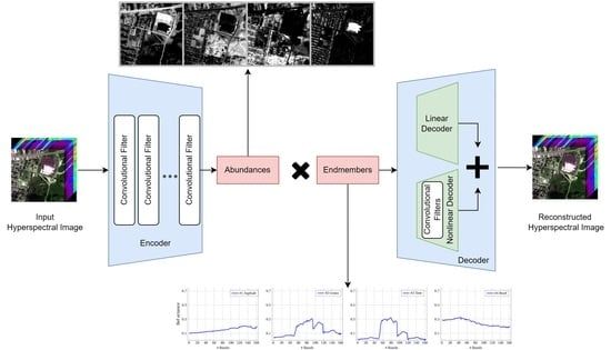
Figure 1.
Representation of hyperspectral unmixing using an autoencoder.
Figure 1.
Representation of hyperspectral unmixing using an autoencoder.
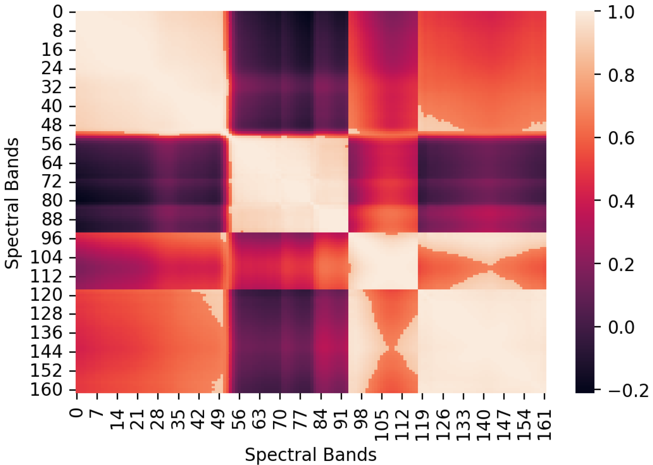
Figure 2.
Heatmap of the correlation matrix of the spectral bands of the Urban Dataset.
Figure 2.
Heatmap of the correlation matrix of the spectral bands of the Urban Dataset.
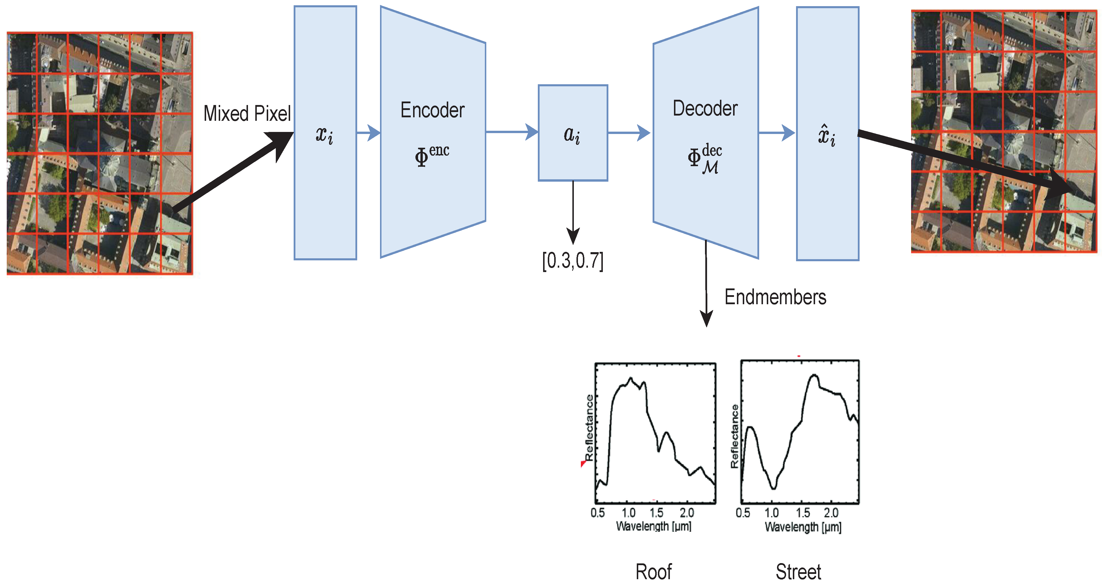
Figure 3.
Diagram of the proposed system.
Figure 3.
Diagram of the proposed system.
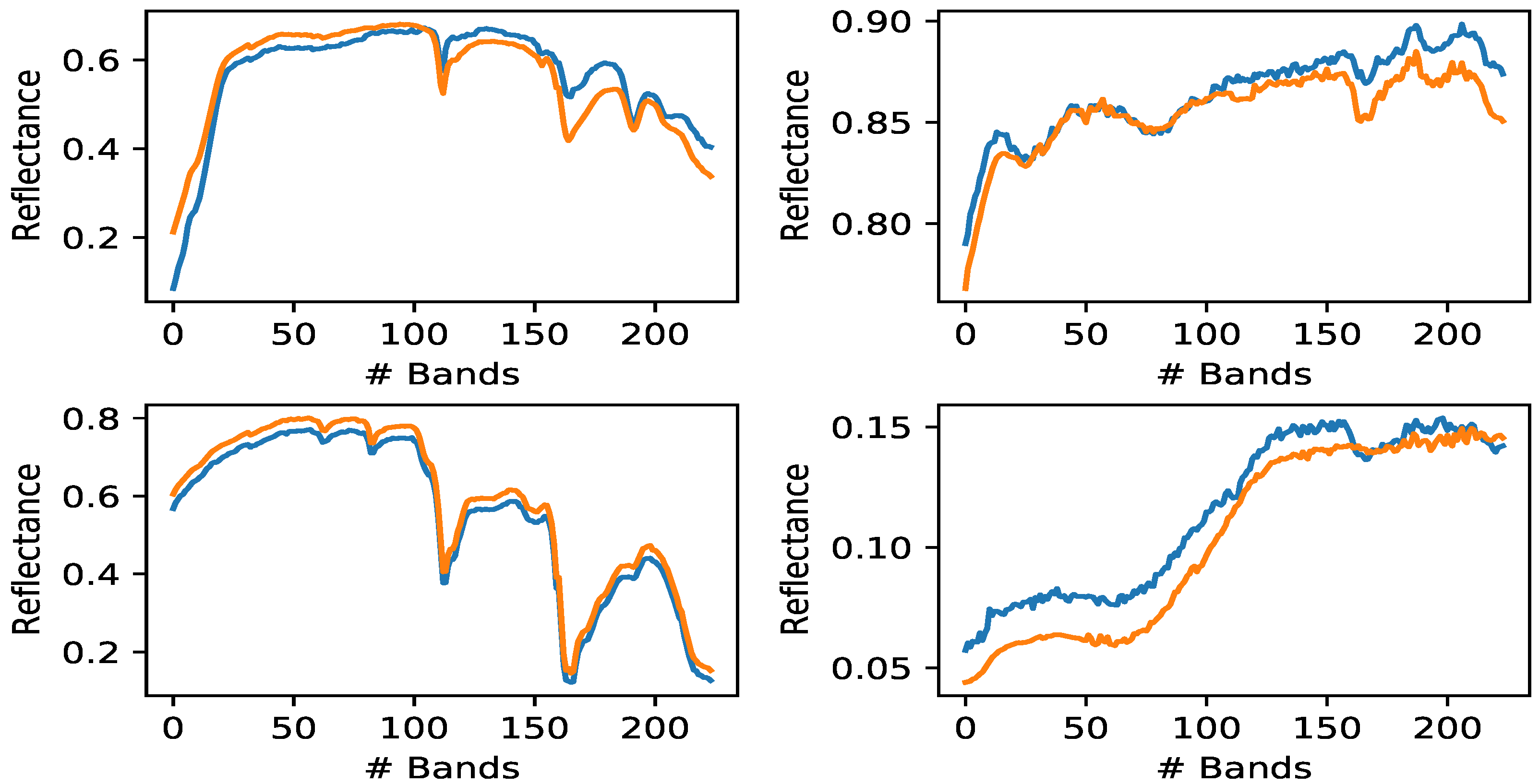
Figure 4.
Comparison between extracted endmembers and the four ground truth synthetic endmembers. Orange curves: true endmembers; Blue curves: extracted endmembers (SNR = 20 dB, bilinear model case).
Figure 4.
Comparison between extracted endmembers and the four ground truth synthetic endmembers. Orange curves: true endmembers; Blue curves: extracted endmembers (SNR = 20 dB, bilinear model case).
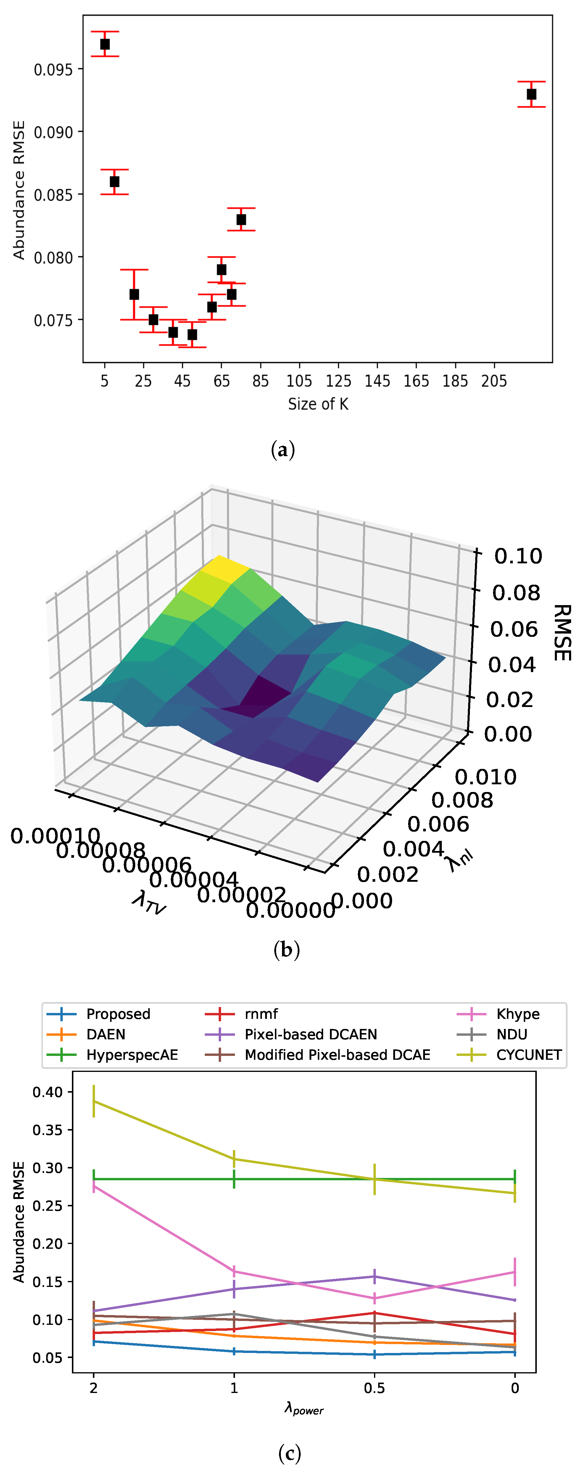
Figure 5.
Model performance as function of regularization parameters and kernel size. (a) Abundance RMSE vs. kernel size K of the proposed model. (b) Abundance RMSE vs. regularization parameters and . (c) Abundance RMSE vs. regularization parameter .
Figure 5.
Model performance as function of regularization parameters and kernel size. (a) Abundance RMSE vs. kernel size K of the proposed model. (b) Abundance RMSE vs. regularization parameters and . (c) Abundance RMSE vs. regularization parameter .
Figure 6.
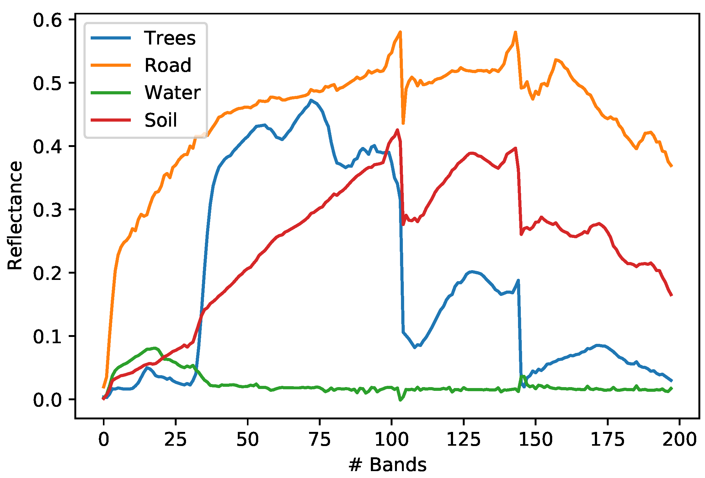
Endmembers extracted by the proposed method for the Jasper Ridge.
Figure 6.
Endmembers extracted by the proposed method for the Jasper Ridge.
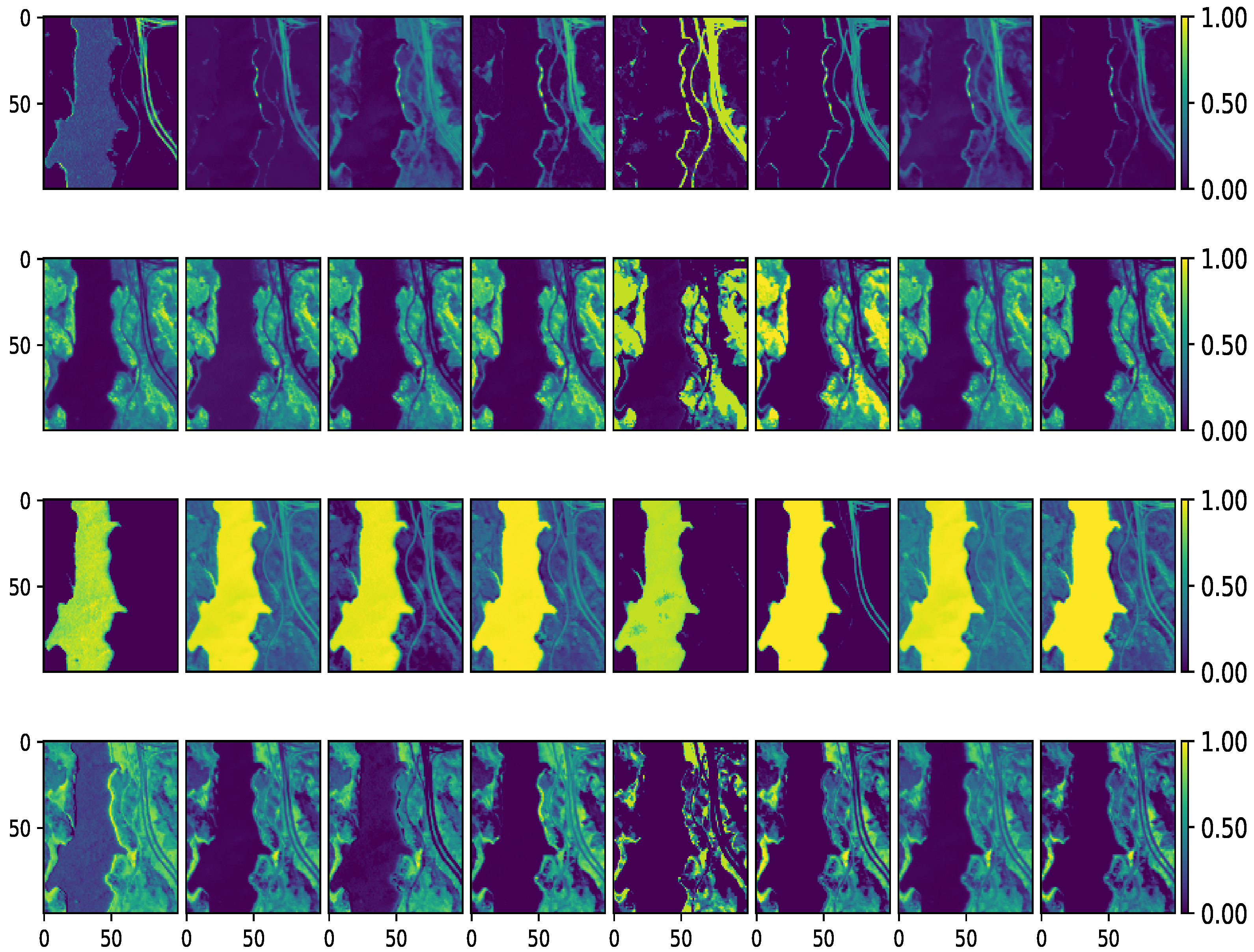
Figure 7.
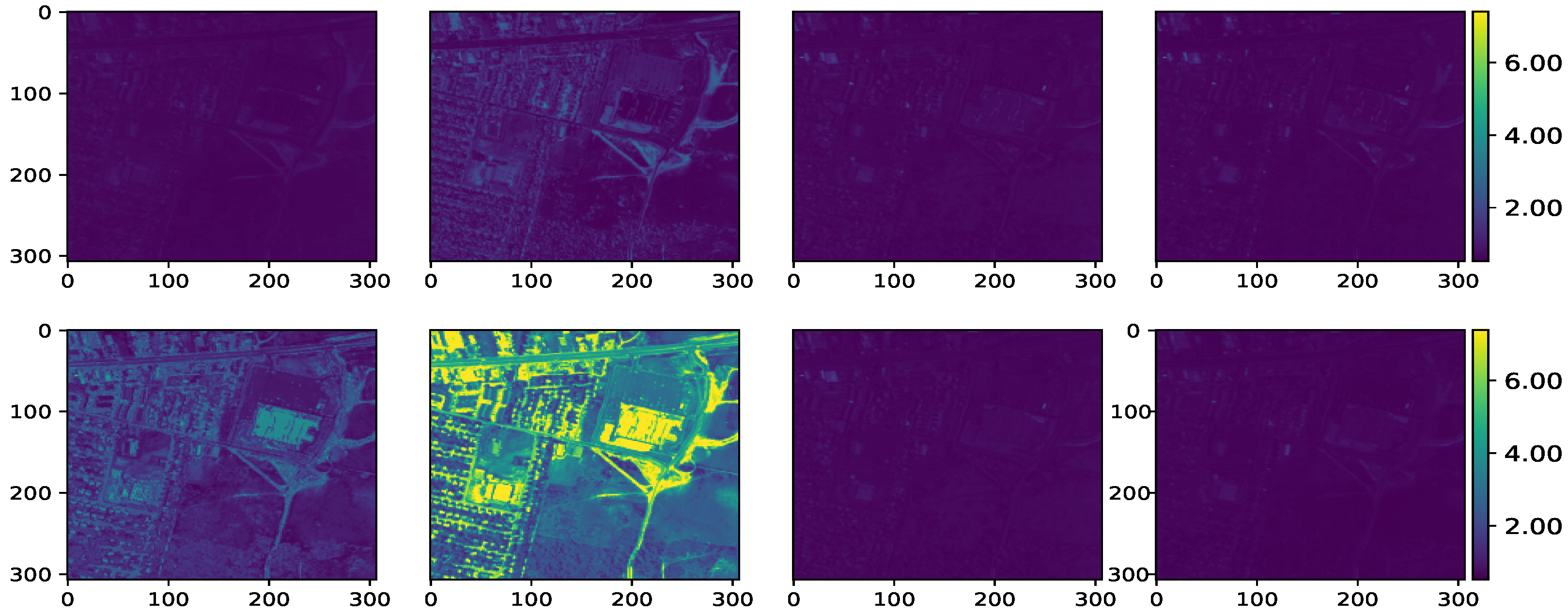
Estimated abundance maps of Jasper Ridge dataset. From left to right: VCA-K-Hype, N-FINDR-NDU, rNMF, DAEN, CYCUNET, Pixel-based DCAE, Modified Pixel-based DCAE, and the proposed method, respectively. From top to bottom: Road, Trees, Water, and Soil, respectively.
Figure 7.
Estimated abundance maps of Jasper Ridge dataset. From left to right: VCA-K-Hype, N-FINDR-NDU, rNMF, DAEN, CYCUNET, Pixel-based DCAE, Modified Pixel-based DCAE, and the proposed method, respectively. From top to bottom: Road, Trees, Water, and Soil, respectively.
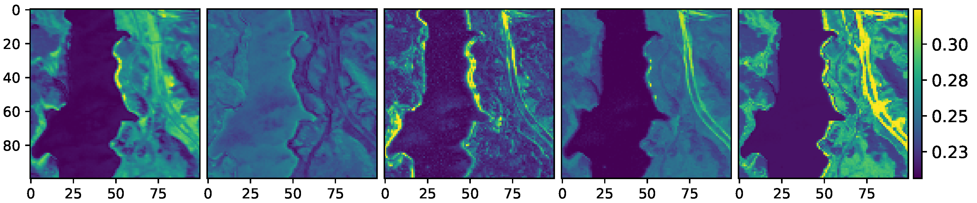
Figure 8.
Energy of the nonlinear components of the Jasper Ridge data. From left to right: VCA-K-Hype, N-FINDR-NDU, rNMF, DAEN, and the proposed method, respectively.
Figure 8.
Energy of the nonlinear components of the Jasper Ridge data. From left to right: VCA-K-Hype, N-FINDR-NDU, rNMF, DAEN, and the proposed method, respectively.
Figure 9.
Maps of reconstruction error of the Jasper Ridge data. From upper left to right: VCA-K-Hype, N-FINDR-NDU, rNMF, DAEN. From bottom left to right: CYCUNET, Pixel-based DCAE, Modified Pixel-based DCAE, and the proposed method, respectively.
Figure 9.
Maps of reconstruction error of the Jasper Ridge data. From upper left to right: VCA-K-Hype, N-FINDR-NDU, rNMF, DAEN. From bottom left to right: CYCUNET, Pixel-based DCAE, Modified Pixel-based DCAE, and the proposed method, respectively.
Figure 10.
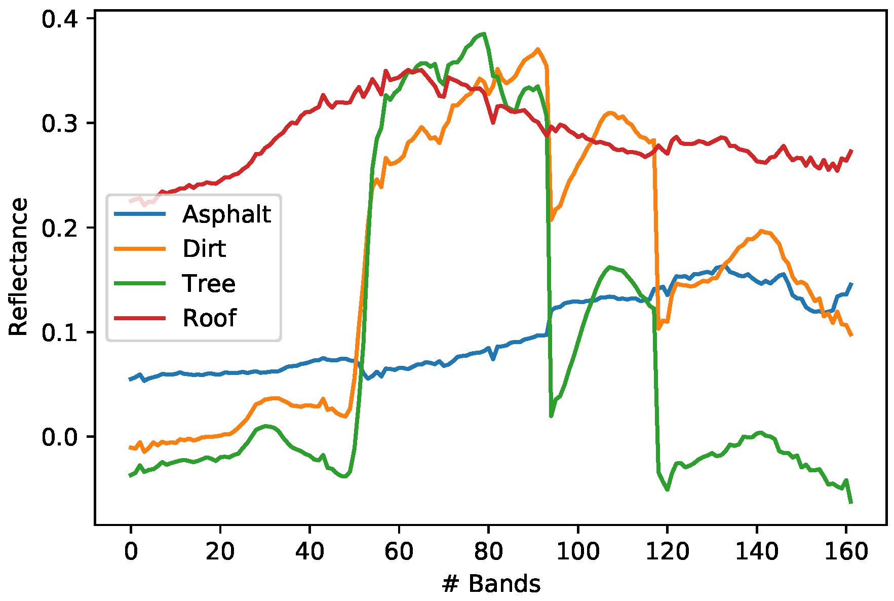
Urban dataset endmembers.
Figure 10.
Urban dataset endmembers.
Figure 11.
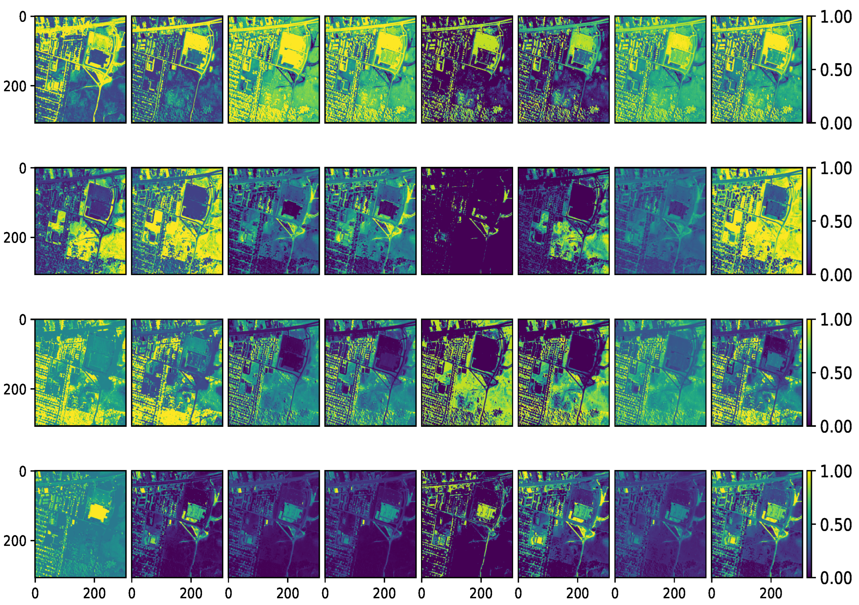
Estimated abundance maps of Urban dataset. From left to right: VCA-K-Hype, N-FINDR-NDU, rNMF, DAEN, CYCUNET, Pixel-based DCAE, Modified Pixel-based DCAE and the proposed method, respectively. From top to bottom: Asphalt, Dirt, Tree, and Roof, respectively.
Figure 11.
Estimated abundance maps of Urban dataset. From left to right: VCA-K-Hype, N-FINDR-NDU, rNMF, DAEN, CYCUNET, Pixel-based DCAE, Modified Pixel-based DCAE and the proposed method, respectively. From top to bottom: Asphalt, Dirt, Tree, and Roof, respectively.
Figure 12.
Energy of the nonlinear components of the Urban data. From left to right: VCA-K-Hype, N-FINDR-NDU, rNMF, DAEN and the proposed method, respectively.
Figure 12.
Energy of the nonlinear components of the Urban data. From left to right: VCA-K-Hype, N-FINDR-NDU, rNMF, DAEN and the proposed method, respectively.
Figure 13.
Maps of reconstruction error of the Urban data. From upper left to right: VCA-K-Hype, N-FINDR-NDU, rNMF, DAEN. From bottom left to right: CYCUNET, Pixel-based DCAE, Modified Pixel-based DCAE, and the proposed method, respectively.
Figure 13.
Maps of reconstruction error of the Urban data. From upper left to right: VCA-K-Hype, N-FINDR-NDU, rNMF, DAEN. From bottom left to right: CYCUNET, Pixel-based DCAE, Modified Pixel-based DCAE, and the proposed method, respectively.
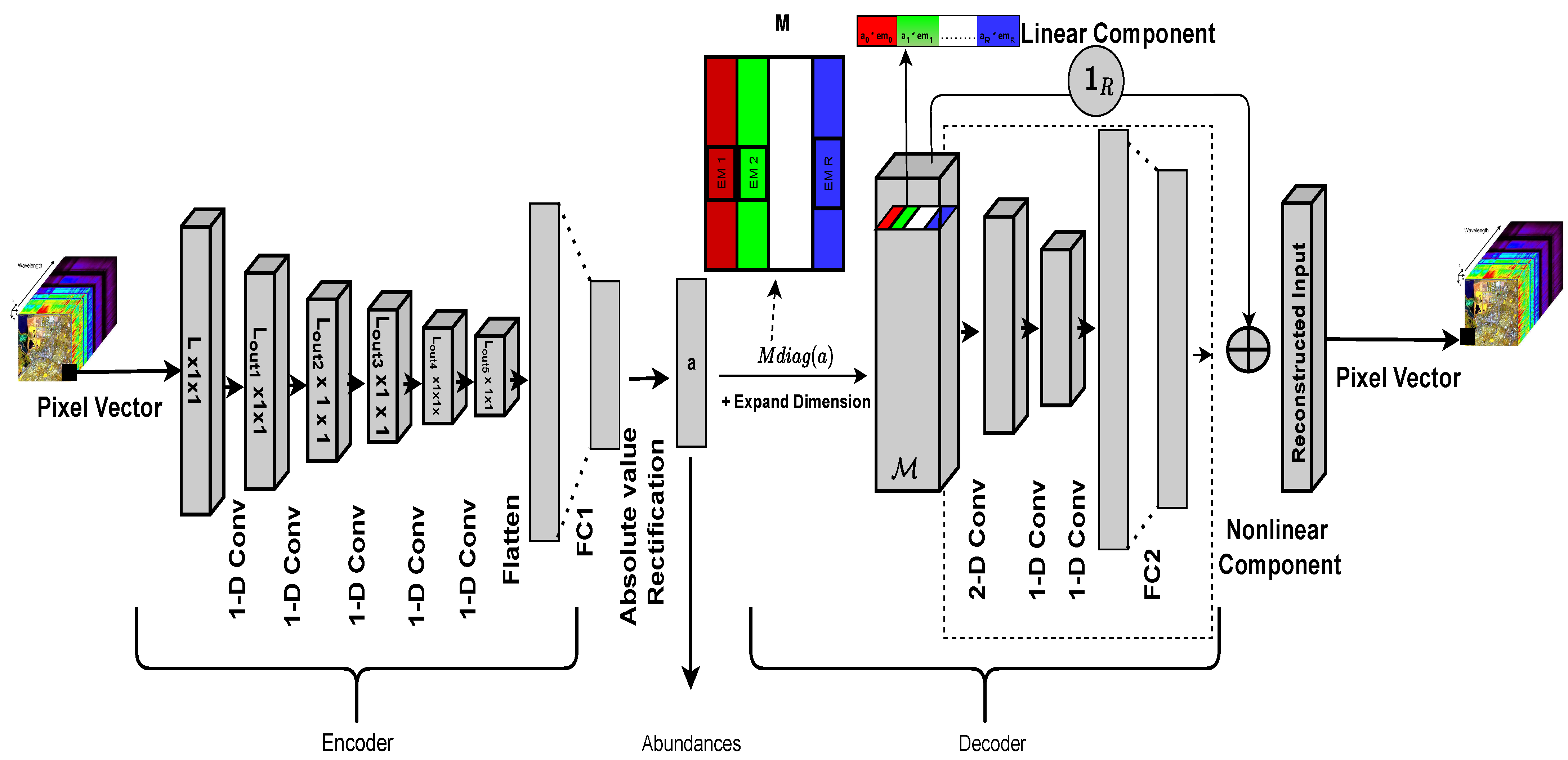
Table 1.
Architecture of the proposed network.
Table 1.
Architecture of the proposed network.
| | Layers | Number of Filters | Size of Each Filter | Activation Function | Pooling | Output Size |
|---|
| Encoder | 1-D Conv | 16 | | ReLU | Max Pooling | |
| 1-D Conv | 32 | | ReLU | Max Pooling | |
| 1-D Conv | 64 | | ReLU | Max Pooling | |
| 1-D Conv | 64 | | ReLU | Max Pooling | |
| 1-D Conv | 64 | | ReLU | Max Pooling | |
| FC1 | 1 | - | ReLU | - | |
| Absolute Value Rectification | - | - | - | - | |
| Decoder | Linear | 1 | - | ReLU | No | |
| 2-D Conv | 64 | (K, R) | ReLU | No | |
| 1-D Conv | 64 | K | ReLU | No | |
| 1-D Conv | 128 | K | ReLU | No | |
| FC2 | 1 | - | ReLU | - | |
Table 2.
Benchmark methods used for comparison.
Table 2.
Benchmark methods used for comparison.
| Method | Description |
|---|
| VCA & K-Hype | Vertex Component Analysis is a classic
geometric method and K-Hype is a linear/nonlinear fluctuation model that approximates the nonlinearity with the kernel trick [12]. |
| N-FINDR & NDU | N-FINDR is a classic endmember extraction method and NDU performs a nonlinear abundance estimation using neighborhood information [34]. |
| r-NMF | Robust non-negative matrix factorization performs robust nonlinear endmember and abundance estimation via block-coordinate descent algorithm [35]. |
| HyperspecAE | Hyperspectral Linear Unmixing Using A Neural Network Autoencoder [19]. |
| DAEN | Deep autoencoder network for linear/nonlinear fluctuation unmixing [22]. |
| CYCUNET | Cycle-consistency Unmixing Network by Learning Cascaded Autoencoders [36]. |
| Pixel-based DCAE | Deep Convolutional Autoencoder for Linear Hyperspectral Unmixing [18]. |
| Modified Pixel-based DCAE | Deep Convolutional Autoencoder for Linear Hyperspectral Unmixing [18] trained with MSE loss function and in an unsupervised way. |
Table 3.
Abundance RMSE comparison of the synthetic data (best results are highlighted in red).
Table 3.
Abundance RMSE comparison of the synthetic data (best results are highlighted in red).
| | SNR = 20 dB | SNR = 30 dB |
|---|
| | Linear | Bilinear | PNMM | Linear | Bilinear | PNMM |
| NFINDR + NDU | 0.0632 ± 0.0045 | 0.1073 ± 0.0023 | 0.0801 ± 0.0034 | 0.0593 ± 0.0074 | 0.0889 ± 0.0033 | 0.0794 ± 0.0062 |
| VCA + K-Hype | 0.1626 ± 0.0185 | 0.1634 ± 0.0077 | 0.1607 ± 0.0186 | 0.0674 ± 0.0050 | 0.0782 ± 0.0033 | 0.1113 ± 0.0097 |
| rNMF | 0.0808 ± 0.0107 | 0.0871 ± 0.0041 | 0.1127 ± 0.0029 | 0.0824 ± 0.0062 | 0.0859 ± 0.0050 | 0.1142 ± 0.0014 |
| HyperspecAE | 0.2848 ± 0.0122 | 0.2848 ± 0.0123 | 0.2848 ± 0.0126 | 0.2848 ± 0.0131 | 0.2849 ± 0.0135 | 0.2848 ± 0.0138 |
| DAEN | 0.0665 ± 0.0100 | 0.0782 ± 0.0020 | 0.0894 ± 0.0067 | 0.0679 ± 0.0062 | 0.0678 ± 0.0045 | 0.0941 ± 0.0040 |
| CYCUNET | 0.2662 ± 0.0124 | 0.2846 ± 0.0205 | 0.3574 ± 0.0231 | 0.3950 ± 0.0156 | 0.4228 ± 0.0189 | 0.3823 ± 0.0164 |
| Pixel-based DCAE | 0.1255 ± 0.0020 | 0.1407 ± 0.0120 | 0.1431 ± 0.0220 | 0.0563 ± 0.0042 | 0.0611 ± 0.0240 | 0.1216 ± 0.0111 |
| Modified Pixel-based DCAE | 0.2449 ± 0.0112 | 0.0999 ± 0.0116 | 0.0967 ± 0.0107 | 0.2554 ± 0.0072 | 0.2684 ± 0.0104 | 0.1126 ± 0.0108 |
| Proposed method | 0.0571 ± 0.0060 | 0.0578 ± 0.0051 | 0.0614 ± 0.0055 | 0.0578 ± 0.0064 | 0.0578 ± 0.0055 | 0.0586 ± 0.0042 |
| | SNR = 40 dB | | | |
| | Linear | Bilinear | PNMM | | | |
| NFINDR + NDU | 0.0577 ± 0.0082 | 0.0907 ± 0.0026 | 0.0659 ± 0.0070 | | | |
| VCA + K-Hype | 0.0583 ± 0.0029 | 0.0758 ± 0.0027 | 0.0792 ± 0.0104 | | | |
| rNMF | 0.0871 ± 0.0089 | 0.0942 ± 0.0059 | 0.1155 ± 0.0009 | | | |
| HyperspecAE | 0.2848 ± 0.0141 | 0.2849 ± 0.0145 | 0.2848 ± 0.0138 | | | |
| DAEN | 0.0608 ± 0.0067 | 0.0695 ± 0.0065 | 0.0896 ± 0.0042 | | | |
| CYCUNET | 0.3562 ± 0.0185 | 0.3562 ± 0.0241 | 0.4044 ± 0.0217 | | | |
| Pixel-based DCAE | 0.0463 ± 0.0630 | 0.0618 ± 0.0840 | 0.1159 ± 0.0060 | | | |
| Modified Pixel-based DCAE | 0.1134 ± 0.0073 | 0.1037 ± 0.0068 | 0.1009 ± 0.0103 | | | |
| Proposed method | 0.0595 ± 0.0058 | 0.0577 ± 0.0058 | 0.0620 ± 0.0029 | | | |
Table 4.
Endmember SAD comparison of the synthetic data (best results are highlighted in red).
Table 4.
Endmember SAD comparison of the synthetic data (best results are highlighted in red).
| | SNR = 20 dB | SNR = 30 dB | SNR = 40 dB |
|---|
| | Linear | Bilinear | PNMM | Linear | Bilinear | PNMM | Linear | Bilinear | PNMM |
| NFINDR + NDU/ Pixel-based DCAE | 0.0998 | 0.1343 | 0.1675 | 0.0652 | 0.0856 | 0.1544 | 0.0621 | 0.0842 | 0.1534 |
| VCA + K-Hype | 0.0645 | 0.0929 | 0.0991 | 0.0531 | 0.0558 | 0.1066 | 0.0532 | 0.0586 | 0.0951 |
| rNMF | 0.0829 | 0.1016 | 0.1402 | 0.0853 | 0.1081 | 0.1345 | 0.1087 | 0.1098 | 0.1334 |
| HyperspecAE | 0.0989 | 0.1103 | 0.1789 | 0.0852 | 0.1185 | 0.1544 | 0.8215 | 0.1424 | 0.1534 |
| DAEN | 0.0750 | 0.0788 | 0.0904 | 0.0751 | 0.1108 | 0.1014 | 0.0823 | 0.1208 | 0.1133 |
| CYCUNET | 0.1197 | 0.1259 | 0.1547 | 0.0513 | 0.0761 | 0.0894 | 0.03723 | 0.0679 | 0.0758 |
| Modified Pixel-based DCAE | 0.2537 | 0.1060 | 0.1340 | 0.2596 | 0.3347 | 0.1450 | 0.1255 | 0.1032 | 0.1319 |
| Proposed method | 0.0423 | 0.0577 | 0.1193 | 0.0305 | 0.0380 | 0.0905 | 0.0294 | 0.0397 | 0.0919 |
Table 5.
Endmember SID comparison of the synthetic data (best results are highlighted in red).
Table 5.
Endmember SID comparison of the synthetic data (best results are highlighted in red).
| | SNR = 20 dB | SNR = 30 dB | SNR = 40 dB |
|---|
| | Linear | Bilinear | PNMM | Linear | Bilinear | PNMM | Linear | Bilinear | PNMM |
| NFINDR + NDU/ Pixel-based DCAE | 0.0421 | 0.0589 | 0.0641 | 0.0080 | 0.0116 | 0.0189 | 0.0035 | 0.0070 | 0.0116 |
| VCA + K-Hype | 0.0405 | 0.0226 | 0.0109 | 0.0036 | 0.0029 | 0.2405 | 0.0051 | 0.0047 | 0.0133 |
| rNMF | 0.0124 | 0.0128 | 0.0317 | 0.0146 | 0.0140 | 0.0290 | 0.0192 | 0.0146 | 0.0288 |
| HyperspecAE | 0.0625 | 0.0432 | 0.0789 | 0.0765 | 0.0125 | 0.0256 | 0.0081 | 0.0450 | 0.0480 |
| DAEN | 0.0142 | 0.0146 | 0.0272 | 0.0095 | 0.0322 | 0.0546 | 0.0091 | 0.0350 | 0.0470 |
| CYCUNET | 0.0411 | 0.0434 | 0.064 | 0.0079 | 0.0115 | 0.0189 | 0.0034 | 0.007 | 0.0115 |
| Modified Pixel-based DCAE | 0.1201 | 0.1172 | 0.0794 | 0.0793 | 0.1847 | 0.1532 | 0.1793 | 0.1224 | 0.1188 |
| Proposed method | 0.0113 | 0.0095 | 0.0233 | 0.0033 | 0.0047 | 0.0051 | 0.0034 | 0.0058 | 0.0055 |
Table 6.
Re-comparison of the real airborne data (best results are highlighted in red).
Table 6.
Re-comparison of the real airborne data (best results are highlighted in red).
| | RE |
|---|
| Method | Jasper Ridge | Urban |
| KHYPE | 0.0151 ± 0.0009 | 0.0115 ± 0.0002 |
| NDU | 0.0185 ± 0.0009 | 0.0376 ± 0.0003 |
| rNMF | 0.0131 ± 0.0004 | 0.0120 ± 0.0003 |
| HyperspecAE | 0.0877 ± 0.0052 | 0.0702 ± 0.0013 |
| DAEN | 0.01 ± 0.0009 | 0.0059 ± 0.0005 |
| CYCUNET | 0.0303 ± 0.0007 | 0.0764 ± 0.0007 |
| Pixel-based DCAE | 0.0771 ± 0.0009 | 0.229 ± 0.0012 |
| Modified Pixel-based DCAE | 0.0113 ± 0.0003 | 0.0113 ± 0.0003 |
| 3-D-CNN Autoencoder Network (results from [24]) | 0.0118 | 0.0116 |
| Proposed method | 0.0068 ± 0.0002 | 0.0096 ± 0.0002 |
Table 7.
The average computation time for each dataset.
Table 7.
The average computation time for each dataset.
| Method | Time [Sec] |
|---|
| | Synthetic | Jasper | Urban |
| NDU | 1410 | 1380 | 7840 |
| K-Hype | 19 | 25 | 190 |
| rNMF | 90 | 95 | 170 |
| HyperspecAE | 450 | 330 | 950 |
| DAEN | 670 | 492 | 1426 |
| Cycunet | 50 | 52 | 380 |
| Pixel-based DCAE | 590 | 433 | 1255 |
| Modified Pixel-based DCAE | 600 | 441 | 1279 |
|
Proposed method | 650 | 477 | 1383 |


