Deep Learning for InSAR Phase Filtering: An Optimized Framework for Phase Unwrapping

Abstract

Interferometric Synthetic Aperture Radar (InSAR) data processing applications, such as deformation monitoring and topographic mapping, require an interferometric phase filtering step. Indeed, the filtering quality significantly impacts the deformation and terrain height estimation accuracy. However, the existing classical and deep learning-based phase filtering methods provide artefacts in the filtered areas where a large amount of noise prevents retrieving the original signal. In this way, we can no longer distinguish the underlying informative signal for the next processing step. This paper proposes a deep convolutional neural network filtering method, developing a novel learning strategy to preserve the initial phase noise input into these crucial areas. Thanks to the encoder–decoder powerful phase feature extraction ability, the network can predict an accurate coherence and filtered interferometric phase, ensuring reliable final results. Furthermore, we also address a novel Synthetic Aperture Radar (SAR) interferograms simulation strategy that, using initial parameters estimated from real SAR images, considers physical behaviors typical of a real acquisition. According to the results achieved on simulated and real InSAR data, the proposed filtering method significantly outperforms the classical and deep learning-based ones.

1. Introduction

Over the last years, one of the leading remote sensing techniques has been Synthetic Aperture Radar Interferometry (InSAR), which represents one of the best tools to perform complex tasks, such as topography mapping and deformation monitoring. The valuable information about Earth’s surface is encoded using an interferometric phase that exploits the phase difference between two or more Synthetic Aperture Radar (SAR) complex images i.e., the single-look complex (SLC). Like all the coherent imaging systems, SAR images are characterized by an intrinsic noise-like process that depends on several physical phenomena, such as the scattering mechanism, acquisition geometry, sensor parameters and target temporal decorrelation [1,2]. Other artefacts, such as those generated by atmospheric conditions, do not generate coherence loss, and they are not considered here. This noise affects the interferometric phase measurement and makes phase filtering an essential procedure for the whole processing pipeline. Indeed, in order to extract accurate information from the signal, correct phase unwrapping procedures must be performed to retrieve the absolute phase value by adding to each pixel multiples of $2\pi$ phase values. Therefore, good phase detail features preservation (e.g., the fringes and edges) is required during the noise filtering to ensure the measurement accuracy in the subsequent processing steps. In addition to the filtering process, the coherence maps must be accurately estimated. In fact, based on the correlation degree information provided by the coherence, we can select a set of reliably filtered pixels candidates for the phase unwrapping procedure. Thus, interferometric phase filtering and coherence map estimation are fundamental key factors for most InSAR application techniques.

In recent decades, researchers have proposed several approaches to estimate both the interferometric phase and coherence map. The most common phase filtering techniques can be categorized into four groups: the frequency domain, wavelet domain, spatial domain and non-local (NL) methods. Adaptive spatial-domain filters such as Lee [3], estimating the phase noise standard deviation and selecting an adaptive directional window, reduce the noise while achieving a compromise between the loss of the fringe details and the residual noise. Several improved versions have appeared after following the basic Lee filter [4,5,6,7]. However, this window processing operation that tries to increase the ability to maintain the phase detail brings excessive smoothing and curved fringes distortion.

Goldstein and Werner proposed the first frequency-domain method [8], which tries to suppress phase noise, enhancing the signal power spectrum. To increase the overall performance, one of its improvements [9] presented a technique for regulating the filtering intensity by predicting the dominant component from the signal’s local power spectrum. Further modifications have been introduced to create a filtering parameter based on the coherence value to enhance the filtering capacity for low-coherence areas. However, all the frequency-domain filtering approaches always result in a loss of phase details as they suppress the high-frequency components of the fringes. Furthermore, the accuracy of the power spectrum estimation, which determines the performance of the frequency-domain filters, always relies on the phase noise and window size considered.

The first wavelet-domain filter approach (WInPF) based on a complex phase noise model is proposed by Lopez-Martinez and Fabregas [10]. The performance obtained has demonstrated that the spatial-domain approach has a more robust ability to reduce noise, while the wavelet-domain filters have a higher capability to maintain phase details. Following the basic idea of the WInPF, several adapted versions appear [11,12], where the implementation of the Wiener filter, simultaneous detection or estimation techniques helps achieve a better filtering performance and excellent spatial resolution preservation. The result shows that the noise separation from the phase information can be more facilitated in the wavelet domain.

Finally, more recent non-local phase filtering methods have been successfully applied to overcome the limitation imposed by using a local window during the phase estimation and providing effective noise suppression while maintaining better spatial details. Non-local filtering’s main idea is to extract additional details from the data by looking for similar pixels before filtering. More precisely, a patch-similarity criterion assigns a weight to each pixel based on a similarity measurement to the reference pixel. Therefore, each pixel is chosen by evaluating a distance metric that does not consider any spatial proximity criteria. Starting from the patch-based image denoising estimator proposed in [13], Deledalle et al. [14] presented an iterative method based on a probabilistic approach that relies on the intensities and interferometric phases around two specified patches. In particular, the patch-based similarity criterion is applied to compute a membership value, which is then employed in a weighted maximum likelihood estimator (WMLE) to create the appropriate parameters. Finally, the similarity values between the parameters of the pre-estimated patches are included to refine the estimation iteratively. As a further development, Deledalle proposed NL-InSAR [15], the first InSAR application to estimate the interferometric phase, reflectivity and coherence map together from an interferogram using a non-local method.

The non-local state-of-the-art approach is achieved by Sica et al. [16], using the same two-pass strategy as block matching and 3-D filtering [17], in which the second pass was driven by the pilot image created in the first pass. This approach exploits a block-similarity measure, which considers the noise statistics, to create groups of similar patches of a fixed dimension. Then, a collaborative filtering step is used to produce a denoised version in the wavelet domain, computing the wavelet transform on the whole group. In particular, collaborative filtering is performed using hard thresholding in the first filtering pass. Then, Wiener filtering is performed in the second pass based on prior statistics already computed on the pilot image.

In the last years, the increase in Synthetic Aperture Radar Earth Observation missions, such as TerraSar-X, Sentinel- 1, ALOS and Radarsat, has led to a new scenario characterized by the continuous generation of a massive amount of data. On the one hand, this trend has allowed us to disclose the inadequacy of the classical algorithms in terms of generalization capabilities and computational performance; on the other, it paved the way for the new Artificial Intelligence paradigm, including the deep learning one. A phase filtering technique called PFNet, which uses a DCNNs network, was proposed in [18], and another deep learning approach for InSAR phase filtering was presented in [19]. The state-of-the-art approach for InSAR filtering and coherence estimation is achieved by Sica et al. 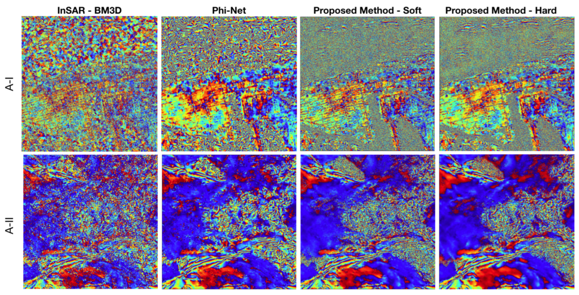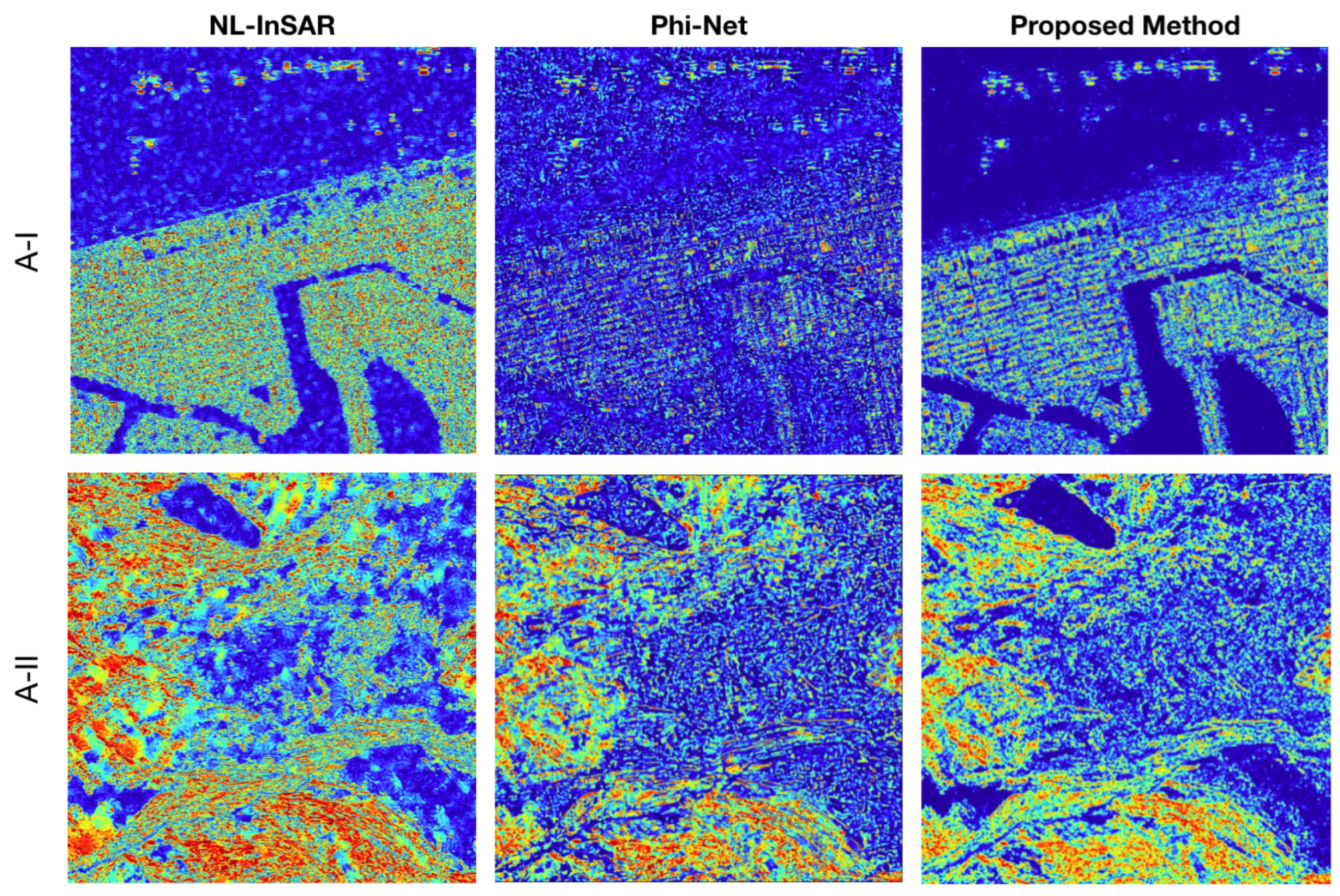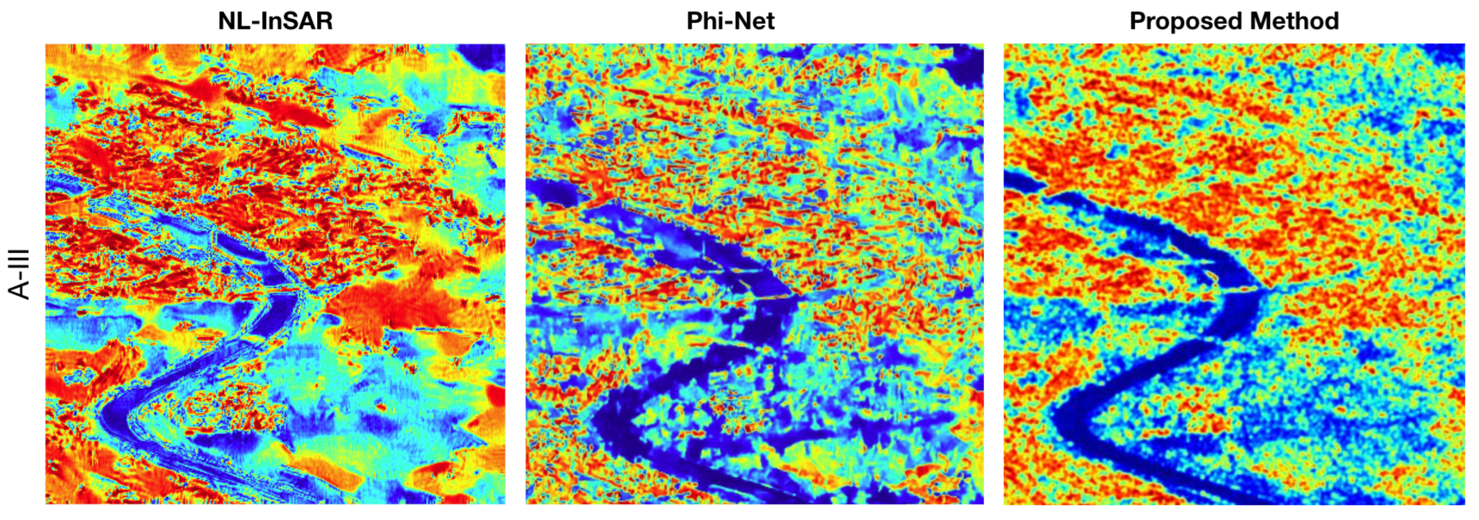[20]. This convolutional neural network (CNN) with residual connections, called Phi-Net, demonstrates the capability of performing denoising working without any prior notions about the input noise power. The network can manage different noise levels, including variations within a single patch. This ensures that distributed spatial patterns, edges and point-like scatterers (which characterize real InSAR data) are localized and well-preserved. However, all the developed methodologies present in the literature generate a wrong filtered signal in areas characterized by a low signal-to-noise ratio (SNR) and high spatial frequency. This behavior does not allow a reliable result that can be used in a phase unwrapping algorithm. This paper proposes a novel deep learning-based methodology for InSAR phase filtering and coherence estimation. In addition to obtaining optimal noise suppression and a retention capacity of phase details, our model addresses the challenging problem of not generating artefacts in the filtered signal. A suitable training stage is developed to preserve the original phase noise input in the areas characterized by a low SNR or high spatial frequency. In this way, we ensure reliable results that can be used to obtain a higher-precision unwrapped phase and ensure computational efficiency. Furthermore, we also address a novel SAR interferograms simulation strategy using the initial parameters from real SAR images. In this way, we created a training dataset that considers the physical behaviors typical of real InSAR data. The experiments on simulated and real InSAR data show that our approach outperforms the state-of-the-art methods present in the literature.

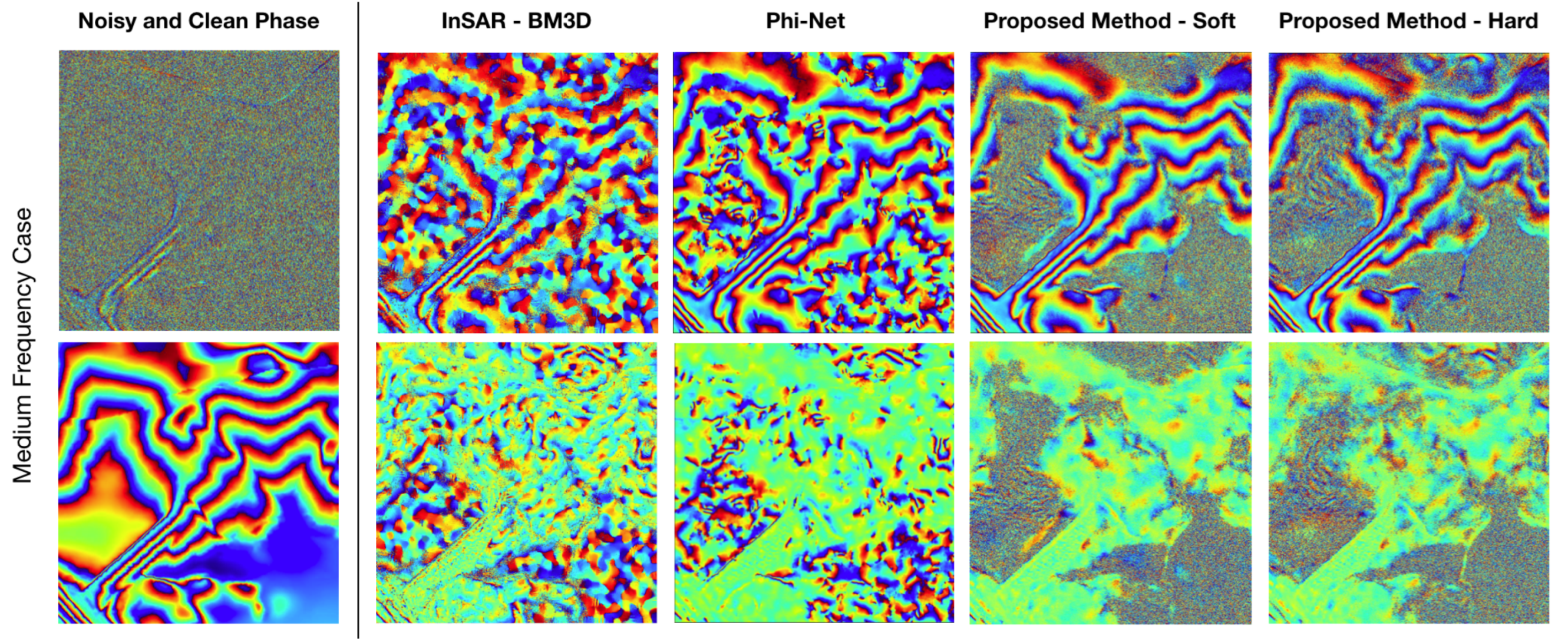
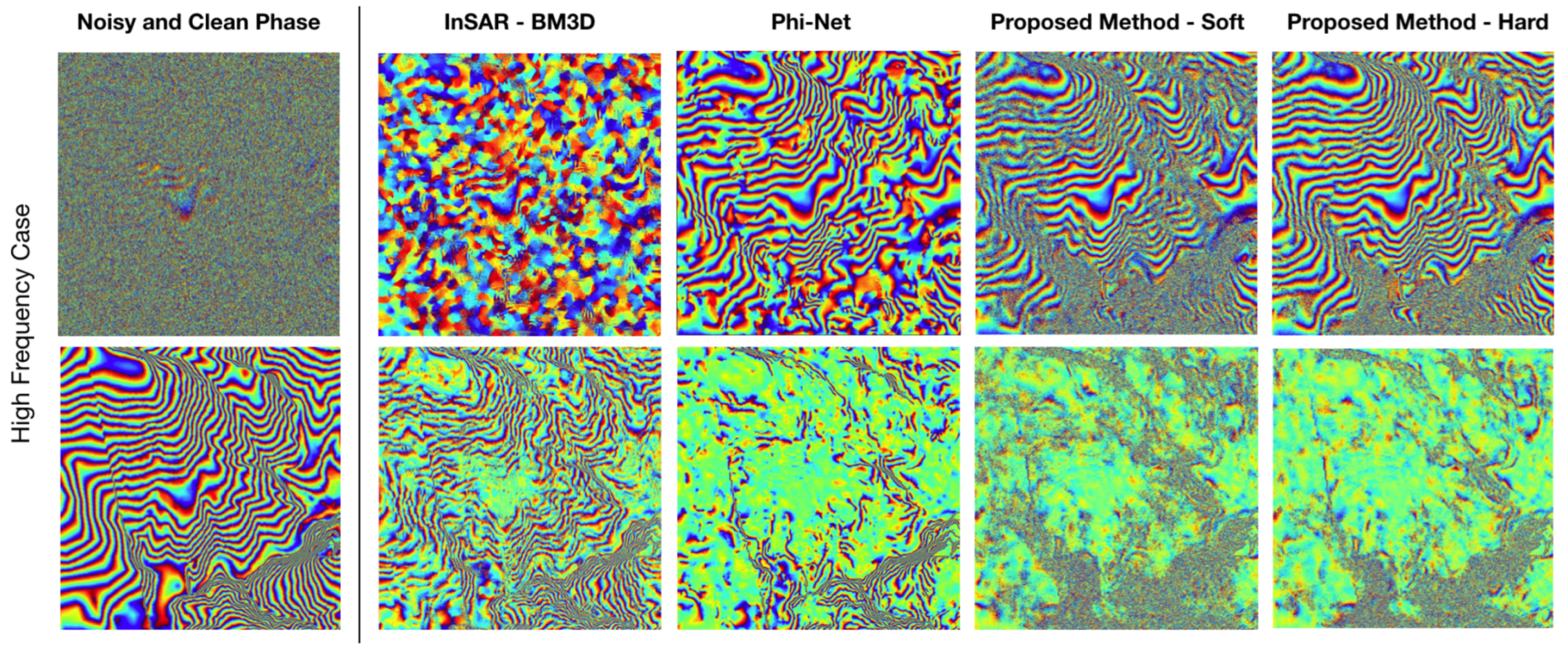
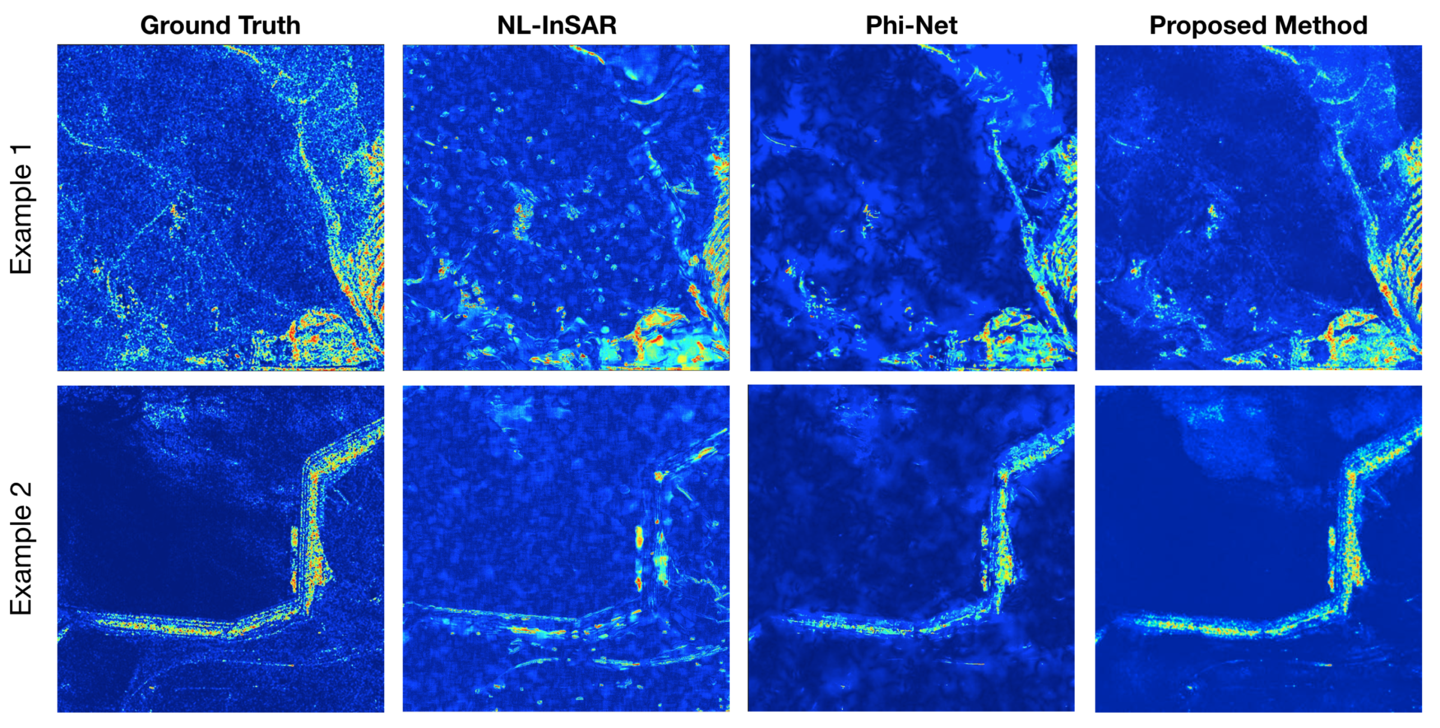
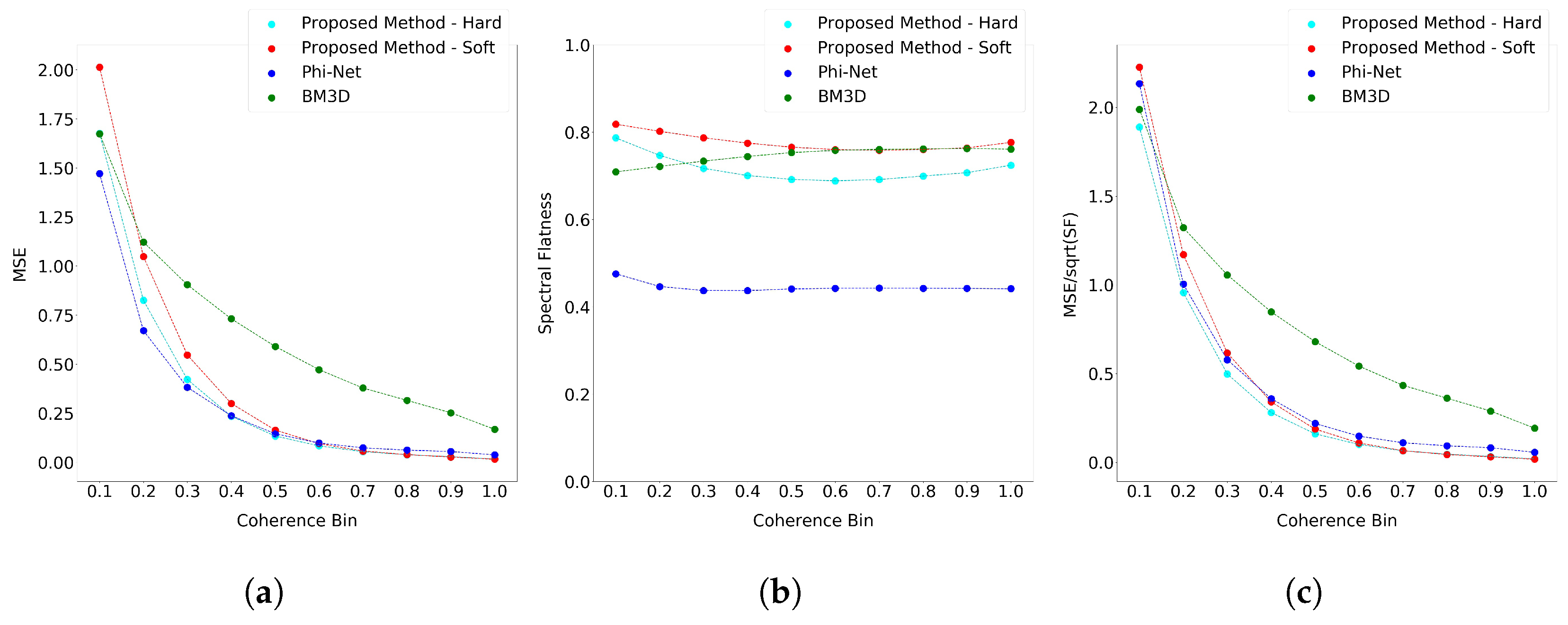
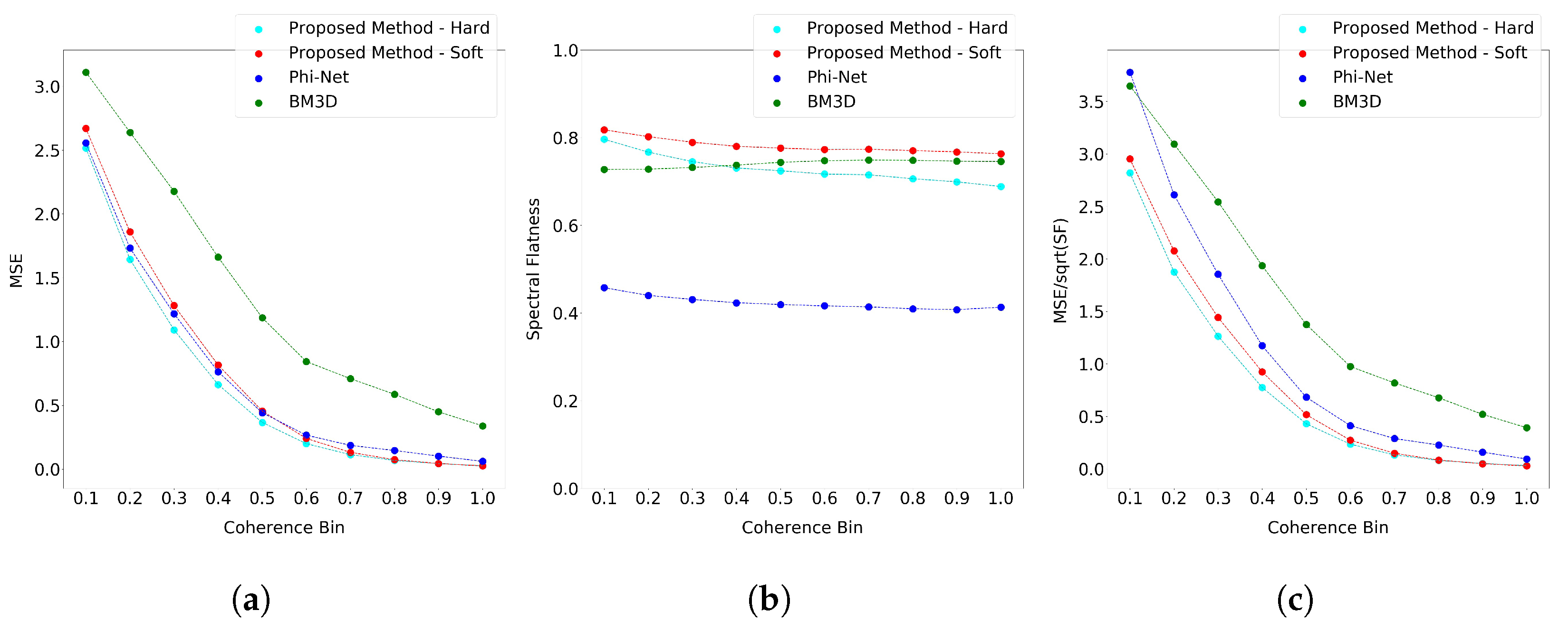
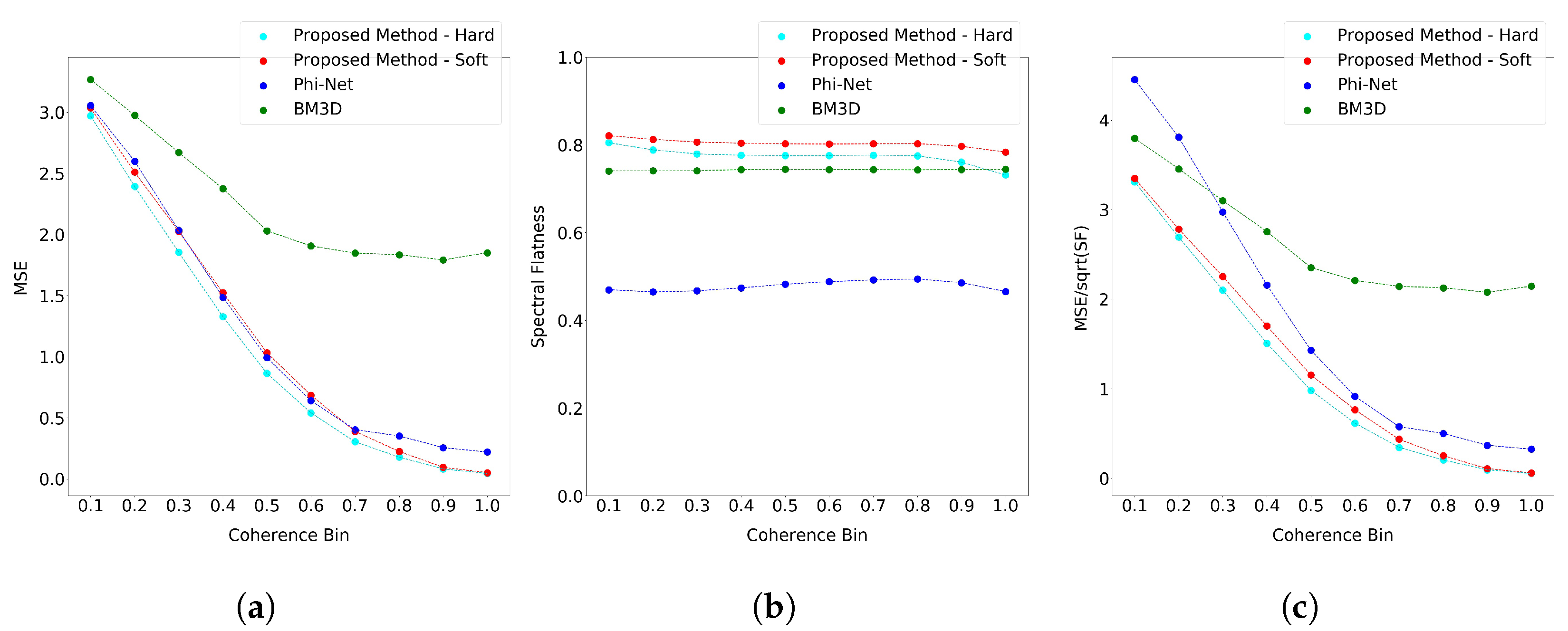
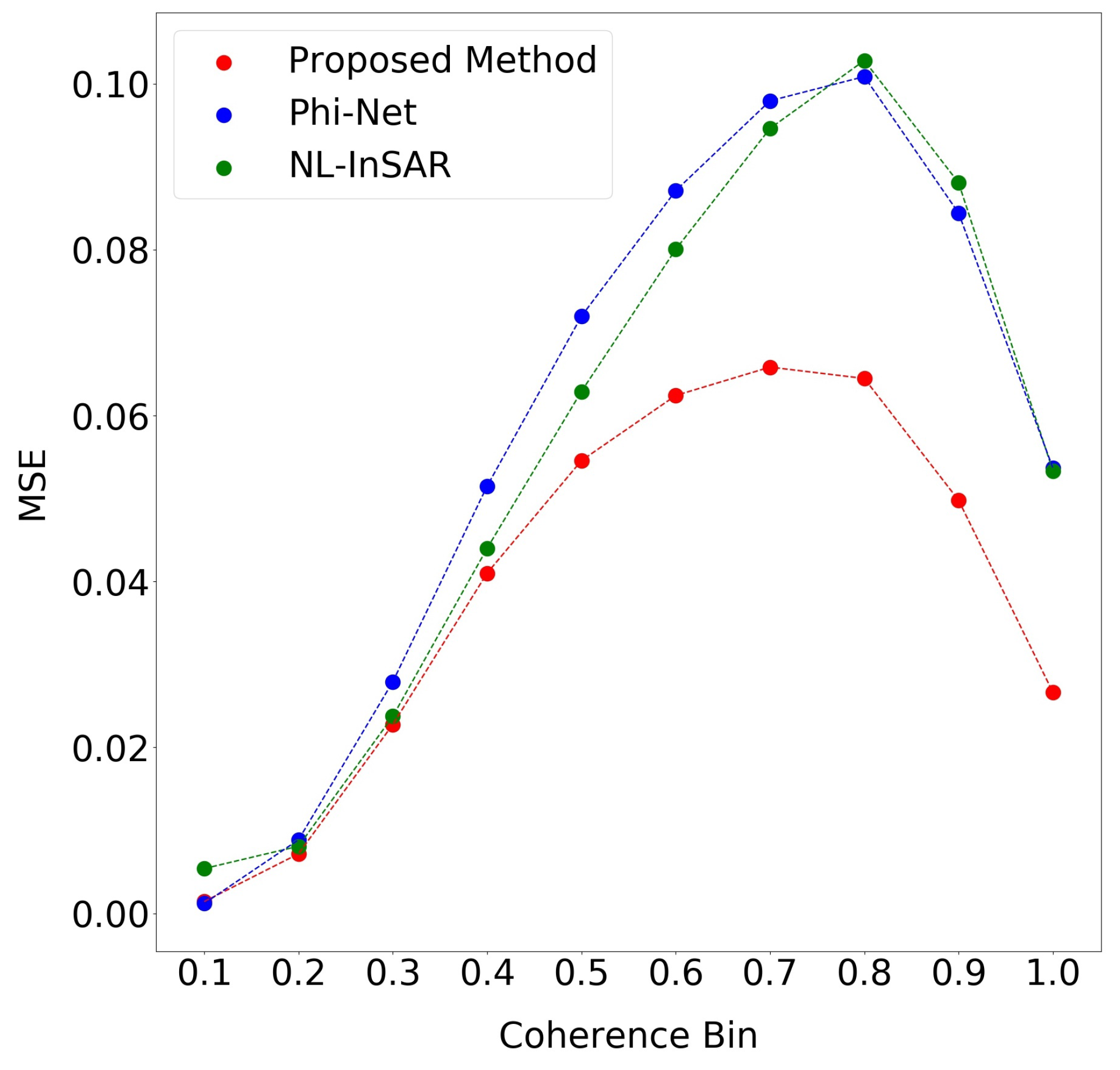
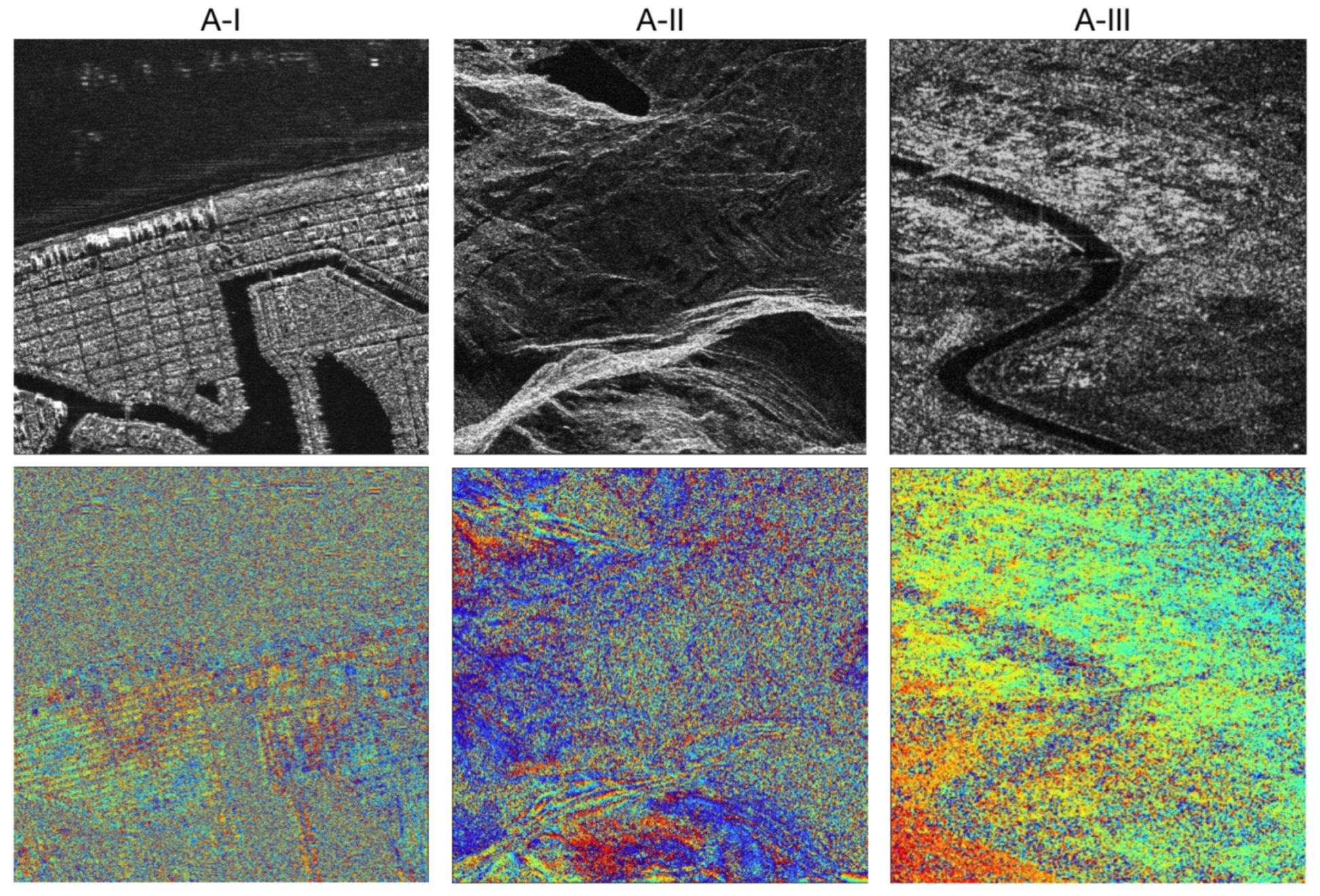
The remaining sections of the paper are structured as follows. Section 2 describes the interferometric phase noise model and the image simulation procedure to generate the synthetic image. The proposed method is introduced in Section 3 by describing the employed architecture and the chosen learning strategy. In Section 4, the simulated and real InSAR data results are presented, comparing the proposed method with four well-established filtering ones. In Section 5, we draw our conclusions and provide potential directions for future research.

2. Model for Data Generation

Deep learning methodologies require the generation of an extensive and reliable training dataset for network learning. Furthermore, a supervised learning framework also requires data-driven procedures, which allows us to evaluate the filtered quality by comparing it with the ground truth. The quality and variety of the training examples have a significant impact on the trained model’s performance. Many InSAR images, together with their noise-free ground truth, are, in fact, necessary to properly train deep learning networks. Fortunately, petabytes of SAR images are now accessible thanks to various Earth Observation missions, such as Sentinel-1, Cosmo-SkyMed, Radarsat and TerraSAR-X. However, having their equivalent noise-free labels is physically impossible. Therefore, synthetically generating the noisy InSAR images is required. In the following subsections, we detail the phase noise model we employed and how it was used to create our semi-synthetic dataset.

2.1. Phase Noise Model

To statistically describe the interferometric SAR signal, we assume that the signal is modeled as a complex circular Gaussian variable, as exploited in [21,22]. The interferogram is calculated by multiplying the complex value of the first SAR SLC image $z_1$, called the master image, by the complex conjugate of the second acquisition $z_2$, called the slave image:

$$\mathsf{\Gamma }=z_1·z_2^{*}$$

(1)

In our model, the interferometric pair ($z_1,z_2$) is computed starting from the two standard circular Gaussian random variables ($u_1,u_2$) as:

$$\left(\genfrac{}{}{0pt}{}{z_1}{z_2}\right)=C\left(\genfrac{}{}{0pt}{}{u_1}{u_2}\right)$$

(2)

where

$$C=\left(\begin{array}{cc}A& 0\\ A\rho e^{-j{\varphi }_c}& A\sqrt{1-{\rho }^2}\end{array}\right)$$

(3)

is the data covariance matrix Cholesky decomposition that depends on the clean interferometric phase ${\varphi }_c$, the coherence $\rho$ and the amplitude A. It should be noted that the amplitude A is assumed to be equal for both the SLC images. The coherence $\rho$ is defined as the amplitude of the correlation coefficient

$$\rho =|\frac{\mathbf{E}\left[z_1{z}_2^{*}\right]}{\sqrt{\mathbf{E}[|z_1{|}^2\left]\mathbf{E}\right[|z_2{|}^2]}}|$$

(4)

and it is a similarity measurement between the two images used to form the interferogram. The more similar the two images reflectivity values are, the higher the interferogram SNR will be (i.e., noiseless interferometric phase).

The interferometric phase noise can be described [3,10] similarly to the typical additive noise model in natural images as

$$\varphi =angle\left(\mathsf{\Gamma }\right)={\varphi }_c+{\varphi }_n$$

(5)

where $\varphi$ is the real interferometric phase, ${\varphi }_c$ is the noise-free interferometric phase and ${\varphi }_n$ is the zero-mean additive Gaussian noise independent from ${\varphi }_c$. It is essential to highlight that, as the interferometric phase observed is modulo $2\pi$ (i.e., wrapped), in order to process it correctly, a complex domain representation must be adopted. According to [10], the complex domain phase noise model can be represented as

$$\begin{array}{c}\hfill x_{real}=cos\left(\varphi \right)=Qcos\left({\varphi }_c\right)+v_r=Q{x}_{c_{real}}+v_r\end{array}$$

(6)

$$\begin{array}{c}\hfill x_{imag}=sin\left(\varphi \right)=Qsin\left({\varphi }_c\right)+v_i=Q{x}_{c_{imag}}+v_i\end{array}$$

(7)

where $x_{real}$ and $x_{imag}$ are real and imaginary parts of the complex interferometric phase $e^{j·\varphi }$, $v_r$ and $v_i$ are the zero-mean additive noise and Q is a quality index monotonically increasing with the coherence $\rho$. In this way, the complex interferogram’s real and imaginary components can be processed individually, allowing us to create an architecture that properly filters the interferometric phase. The estimated clean interferometric phase ${\varphi }_c^{\prime }$ can be reconstructed from filtered real and imaginary parts $x_{c_{real}}^{\prime }$ and $x_{c_{imag}}^{\prime }$ as

$${\varphi }_c^{\prime }=arctan\left(\frac{x_{c_{imag}}^{\prime }}{x_{c_{real}}^{\prime }}\right)$$

(8)

If the phase estimation occurs simply by computing the filtered phase from the corresponding real and imaginary part as just explained, for the coherence estimation, we had to define a second different signal model that would allow us to manage both the phase and coherence data together correctly. Indeed, to obtain a coherence prediction without any estimation bias due to the different values range of the phase and coherence data, we considered the signal model defined as

$$\gamma =\rho ·e^{j·{\varphi }_c}$$

(9)

from which, once the real and imaginary part has been estimated by considering

$$\begin{array}{c}\hfill {\gamma }_{real}=\rho ·cos\left({\varphi }_c\right)\end{array}$$

(10)

$$\begin{array}{c}\hfill {\gamma }_{imag}=\rho ·sin\left({\varphi }_c\right)\end{array}$$

(11)

we can compute the predicted coherence as

$${\rho }^{\prime }=|({\gamma }_{real}^{\prime }+j·{\gamma }_{imag}^{\prime })|$$

(12)

As detailed in Section 3.4, the two signal models presented are then used in the two separate loss functions to estimate phase and coherence, respectively.

2.2. Image Simulation

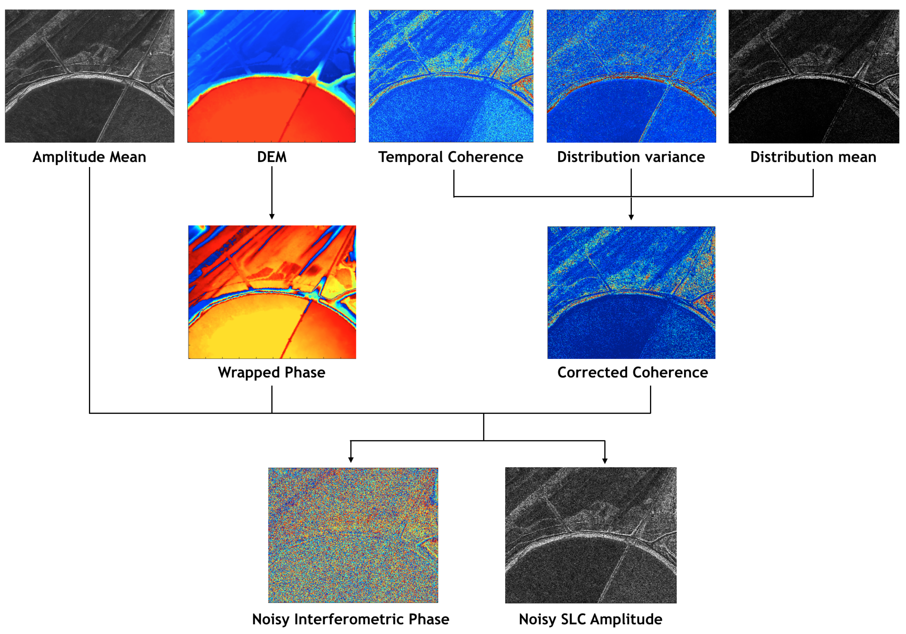
Following the signal model presented in the previous section, we have developed a new SAR interferograms simulation strategy using initial parameters (i.e., amplitude, signal distribution mean and variance, phase and coherence) estimated from real SAR images. As detailed below, we employed an accurate topographic model to generate our semi-synthetic data. Because the parameters are computed over a temporal stack of the same area, the physical relationships among these quantities are intrinsically considered during the data generation process. For instance, a common situation involves an amplitude and interferometric phase that exhibit weakly correlated or uncorrelated patterns, although coherence and amplitude frequently depend on one another. Based on the ground slope and geometric distortions (e.g., layover and foreshortening areas), the interferometric phase typically exhibits patterns with different spatial frequencies. At the same time, the coherence and amplitude may exhibit progressively changing textures, edges and tiny details based on some correlation degree that depends on the characteristics of the acquired area. In addition, abrupt phase changes can occur in areas characterized by powerful scatterers or layover regions. An example could be artificial areas, such as buildings, where coherence and amplitude values are high and phase jumps are due to abrupt changes in the structure’s elevation. In this way, we have obtained a semi-synthetic methodology that can replicate physical behaviors typical of InSAR data and the results provided reliable images regarding amplitude speckle, coherence and interferometric phase noise relationship.

Starting from an external lidar Digital Elevation Model (DEM) with 50 cm resolution, we generate the synthetic topographic wrapped phase ${\varphi }_c$ according to the height-to-phase conversion

$${\varphi }_c=\frac{4\pi }{\lambda }\frac{Bh}{Rsin\left(\theta \right)}$$

(13)

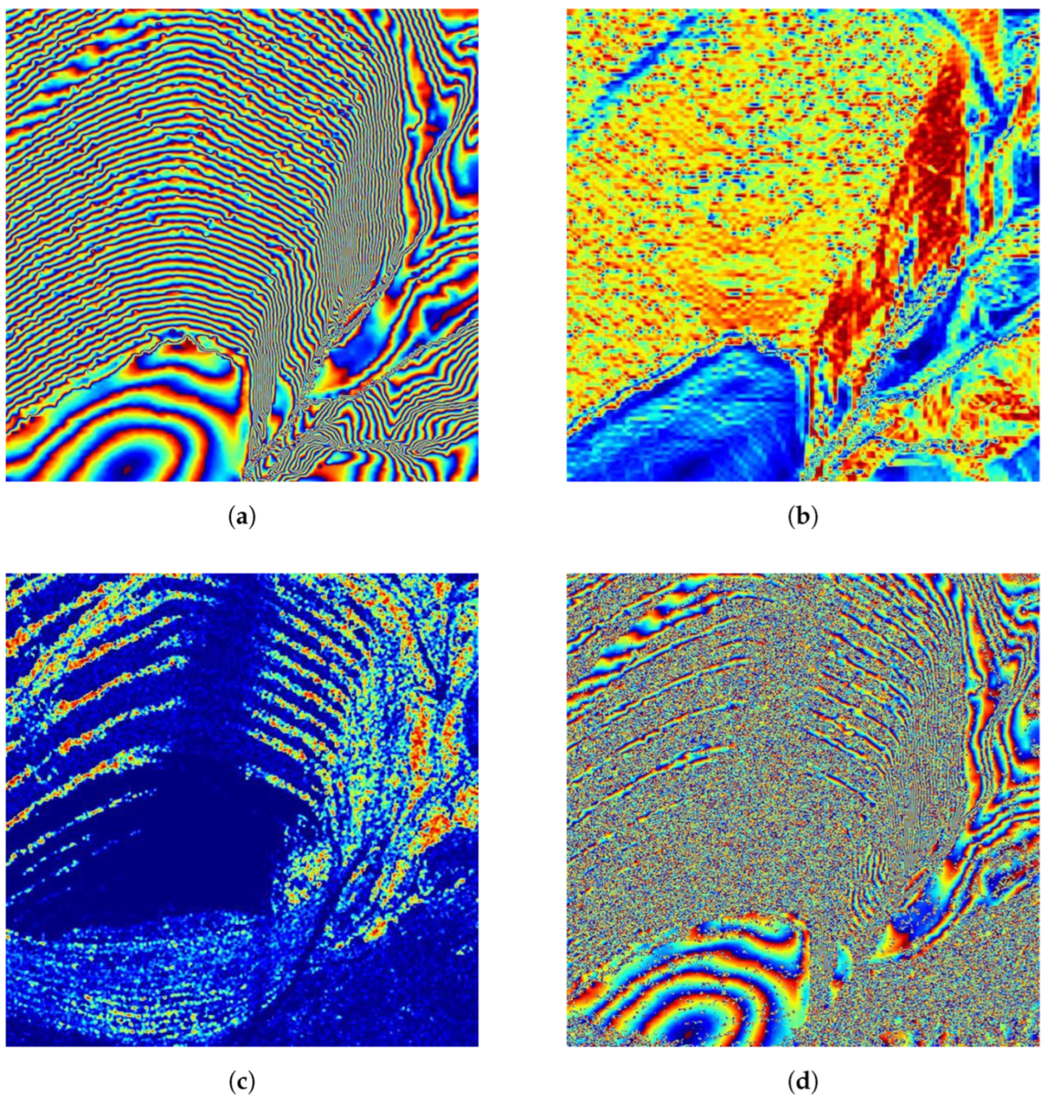
where $\lambda$ is the wavelength of the transmit signal, R is sensor-to-target distance, $\theta$ is the local incidence angle, B is the baseline perpendicular to the line of sight and h is the DEM surface height value. We choose different acquisition geometry parameters to obtain a large variety of training data. Two examples of synthetic interferometric phase patterns are depicted in Figure 1.

As mentioned before, the simulated noisy interferogram $\varphi$ depends on the initial parameters estimated from real acquisitions, i.e., amplitude, signal distribution mean and variance, phase and coherence. Therefore, we first compute the amplitude mean A and the temporal coherence $\rho$ over an image stack of the same area acquired in a different time instant. Then, using a maximum likelihood estimator (MLE), we compute the signal rice distribution mean ${\mu }_{rice}$ and variance ${\sigma }_{rice}^2$ to correct the estimated temporal coherence $\rho$. In particular, we suppose both master and slave images are the sums of two contributions: signal (a, common to both acquisitions) and noise (n, uncorrelated with the signal). Based on Equation (4), it is then easy to compute the coherence:

$$\rho =\left|\frac{\mathbb{E}\left[(a+n_{slave}){(a+n_{master})}^{*}\right]}{\sqrt{\mathbb{E}[|a+n_{slave}{|}^2\left]\mathbb{E}\right[|a+n_{master}{|}^2]}}\right|=\frac{{\sigma }_a^2+{|{\mu }_a|}^2}{{\sigma }_a^2+{|{\mu }_a|}^2+{\sigma }_n^2}$$

(14)

where

$$\mathbb{E}[|n_{slave}{|}^2]=\mathbb{E}[|n_{master}{|}^2]={\sigma }_n^2{\mathrm{and}\mathbb{E}[|a|}^2]={\sigma }_a^2$$

and it is assumed that

$$\left\{\begin{array}{c}\mathbb{E}\left[n\right]=0\hfill \\ \mathbb{E}\left[a\right]={\mu }_a={\mu }_{rice}\hfill \\ {\sigma }_a^2+{\sigma }_n^2={\sigma }_{rice}^2\hfill \\ \mathbb{E}[n_{slave}·n_{master}]=\mathbb{E}\left[n_{slave}\right]\mathbb{E}\left[n_{master}\right]\hfill \\ \mathbb{E}[a·n]=\mathbb{E}\left[a\right]\mathbb{E}\left[n\right]=0\hfill \end{array}\right.$$

Deriving ${\sigma }_a^2$ from Equation (14) and imposing:

$$\left\{\begin{array}{c}{\sigma }_a^2=(\rho -1){|{\mu }_{rice}|}^2+\rho {\sigma }_{rice}^2\hfill \\ {\sigma }_a^2\ge 0\hfill \end{array}\right.$$

(15)

we obtain the following coherence correction rule:

$$\rho \ge \frac{|{\mu }_{rice}{|}^2}{|{\mu }_{rice}{|}^2+{\sigma }_{rice}^2}$$

(16)

In this way, we retrieve the amplitude–coherence degree of interdependence according to the nature of the imaged scene. Before the correction, we also introduce a smoothing factor to the coherence $\rho$ using 3 × 3 box blur filtering. Note that an averaging over more than one point in space is required to estimate spatial coherence. Therefore, as it is impossible to have a pixel-wise estimate resolution, the smoothing factor allows overcoming the estimation limits imposed by considering a 1 × 1 window from which the initial temporal coherence was computed. Finally, we can quickly obtain a pair of randomly simulated SLC SAR images $z_1$ and $z_2$ according to Gaussian model in Equations (2) and (3) using the previously estimated parameters A, ${\varphi }_c$ and $\rho$. Figure 2 shows the processing steps employed to simulate interferogram images. It should be pointed out that several factors affect the coherence, such as baseline, scattering mechanism, SNR, Doppler, volume scattering and temporal decorrelation. Trying to model all the possible noise sources properly is quite challenging as a lot of information over the considered area is required. However, in our methodology, the coherence values used to generate the Gaussian noise are evaluated considering several real images acquired over the area. Therefore, those coherence values take into account all the possible noise sources that can affect an interferogram.

2.3. Model Input

Starting from each pair of simulated SLC SAR images $z_1$ and $z_2$, we extract the interferometric phase $\varphi$ as

$$\varphi =angle\left(z_1{z}_2^{*}\right)$$

(17)

As for the other methods in the literature [18,19,20], we have no requirements and conditions to use the proposed architecture. Our model inputs are the real and imaginary part of the phase together with the normalized image amplitudes:

$$\begin{array}{c}\hfill x_{real}=cos\left(\varphi \right)\end{array}$$

(18)

$$\begin{array}{c}\hfill x_{imag}=sin\left(\varphi \right)\end{array}$$

(19)

$$\begin{array}{c}\hfill A_1=normalize\left[abs\left(z_1\right)\right]\end{array}$$

(20)

$$\begin{array}{c}\hfill A_2=normalize\left[abs\left(z_2\right)\right]\end{array}$$

(21)

In real-world SAR images, the amplitude values range could be extremely broad and may vary across different target sites and radar sensors. In addition, as suggested in several deep learning studies [23,24], the learning-based method requires similar input distribution with low and controlled variance. Hence, as already introduced in [19], all amplitude values are normalized using an adaptive approach to fit into the range [0–1]. The model preserves the original image dynamics while saturating potential outliers without deleting any crucial backscatter information. As presented in [25], we compute the modified Z score using the sample median and Median Absolute Deviation (MAD). In particular, we first calculate the MAD value related to the amplitude image $A_i$ as:

$$MAD=median(|A_i-A_{dataset}|)$$

(22)

where $A_{dataset}$ is the amplitude median computed over the whole dataset. We then transform the data into the modified Z-score domain:

$$A_i^{mz}=\frac{0.6745\ast (A_i-A_{dataset})}{MAD}$$

(23)

$A_i^{mz}$ represents the pixel-wise modified Z score, and the constant 0.6745 is a fixed number computed by the author in [25] to approximate the standard deviation. In this way, we force all potential outliers to be far from 0. Finally, a non-linear function, i.e., tanh, is applied to give a standard input data distribution for network training:

$$A_i^{norm}=\frac{1}{2}(tanh\left(\frac{A_i^{mz}}{W}\right)+1)$$

(24)

where W is a threshold for outlier detection. Data points with $A_i^{mz}$ score greater than W are potential outliers to be ignored [25]. We further normalize the transformed data to the range [0, 1].

3. Proposed Method

All the methodologies present in the literature, inspired by the principles of denoising autoencoders [26,27], addressed the filtering problem by learning a mapping between the interferometric phase real and imaginary part and their corresponding noise-free reconstructions. However, this approach, which has obtained the best performances in natural images, cannot be used in the same way for filtering the interferometric phase images.

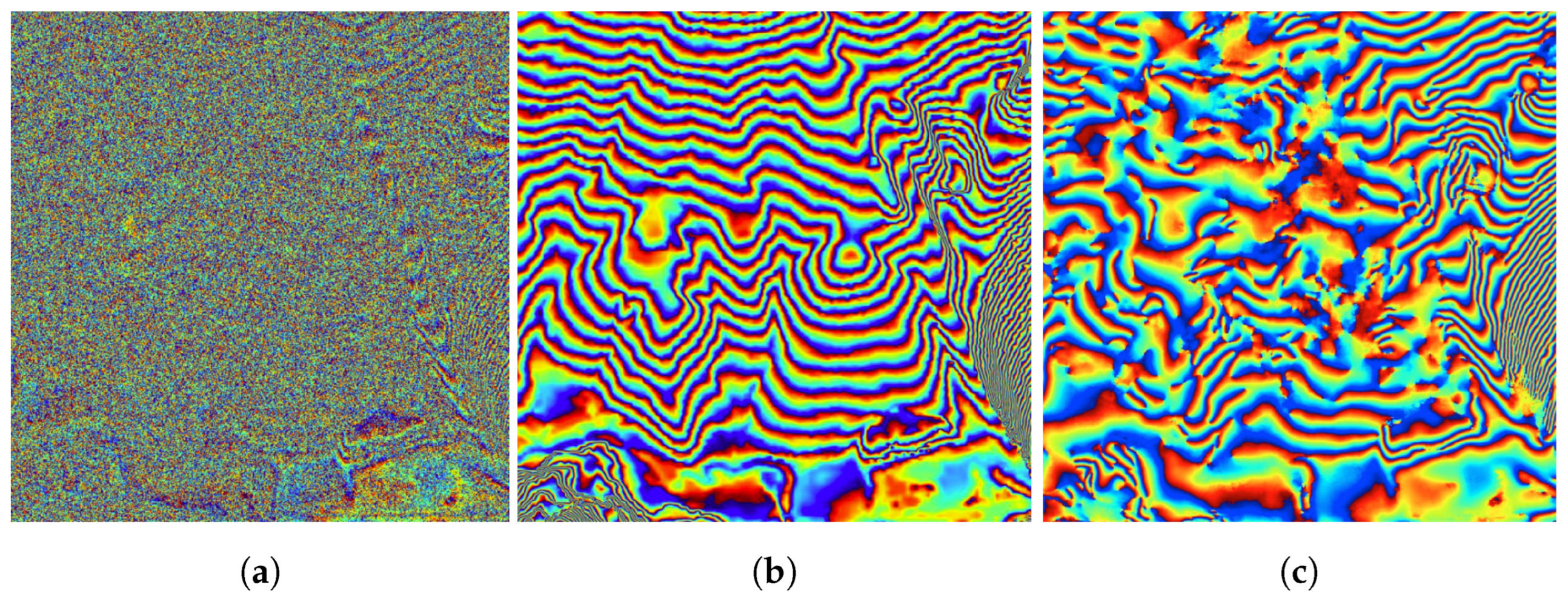
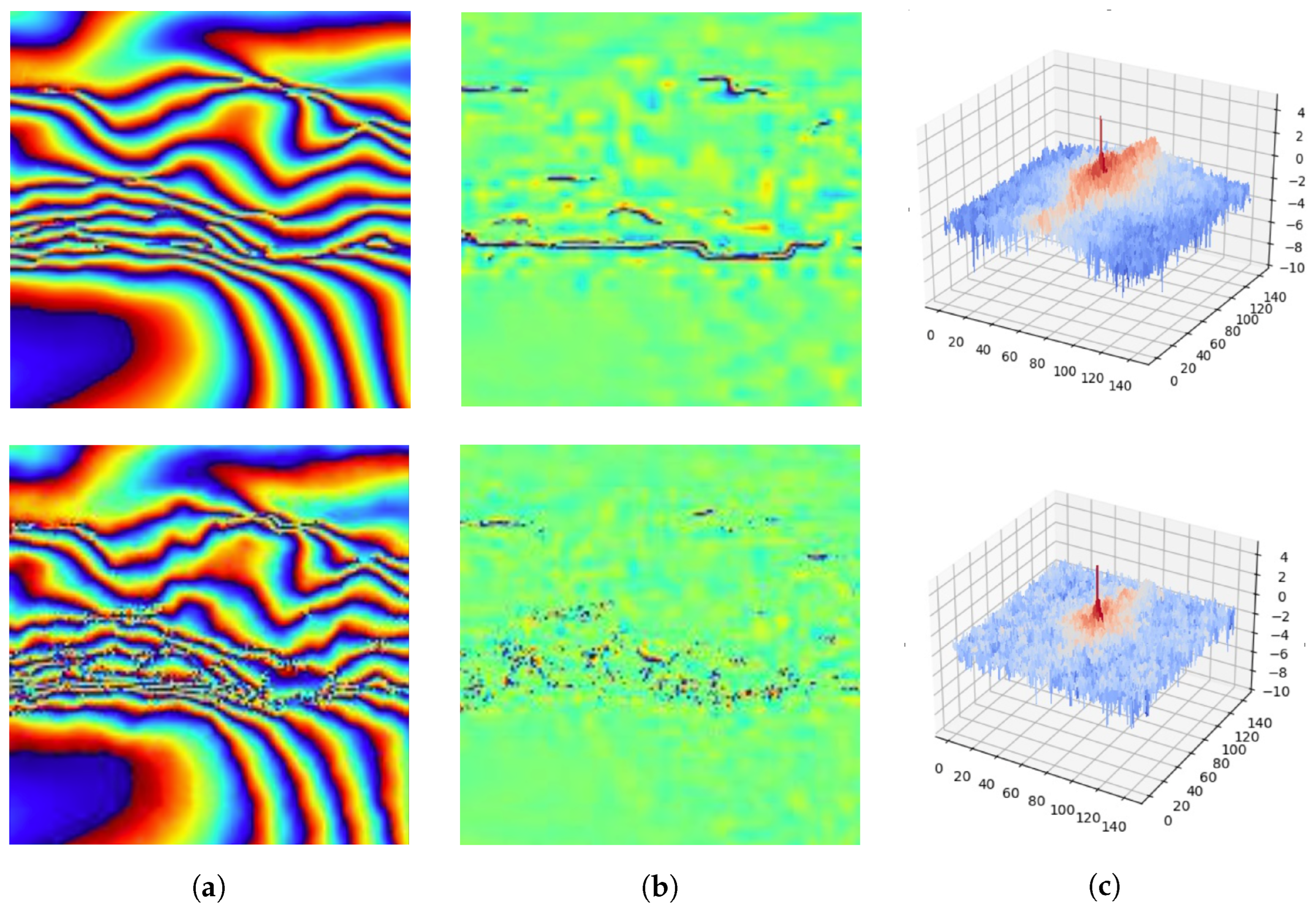
Indeed, some InSAR phase images are affected by low-coherence areas in which a low SNR makes it impossible to retrieve the original signal. Furthermore, there may be very high frequency phase areas in which the fringes are very close to each other, and a small amount of noise is enough not to be able to reconstruct them. Figure 3 shows an example of a wrong filtered signal typical of the state-of-the-art deep learning-based methodologies.

We have developed a modified U-Net version that addresses the challenging problem of not generating artefacts in the reconstructed signal. In this way, we obtain a reliable filtering result that is fundamental in any phase unwrapping algorithm. Indeed, during phase unwrapping, the false phase jumps introduced by the artefacts cause an incorrect wrap count, and these errors propagate over the whole image. Thus, a suitable training stage is developed to preserve the original phase noise input in the areas characterized by low SNR or high spatial frequency.

As mentioned before, we implemented a modified UNet, which is an encoder–decoder convolutional neural network initially employed for semantic segmentation in medical images [28]. It is an architecture designed to learn a model in an end-to-end setting. The UNet’s encoder path compresses the input image information by extrapolating relevant features computed at different resolution scales. As a result, various representations of abstraction levels are provided by this hierarchical feature extraction. On the other hand, the UNet’s decoder path reconstructs the original image by mapping the intermediate representation back to the input spatial resolution. In particular, during this reconstruction process, the information is restored at different resolutions by stacking many upsampling layers. However, when a deep network is employed, some information may be lost during the encoding process, thus making it impossible to retrieve the original image details from its intermediate representation. To address this issue, U-Net implemented a series of skip connections that allow relevant information to be preserved during the decoding stage. In this way, the reconstructed image accuracy can be well preserved. In the following, we describe the changes made to the standard UNet to adapt the network for processing SAR images, and we introduce the learning stage for InSAR phase filtering and coherence estimation.

3.1. Convolutional Block

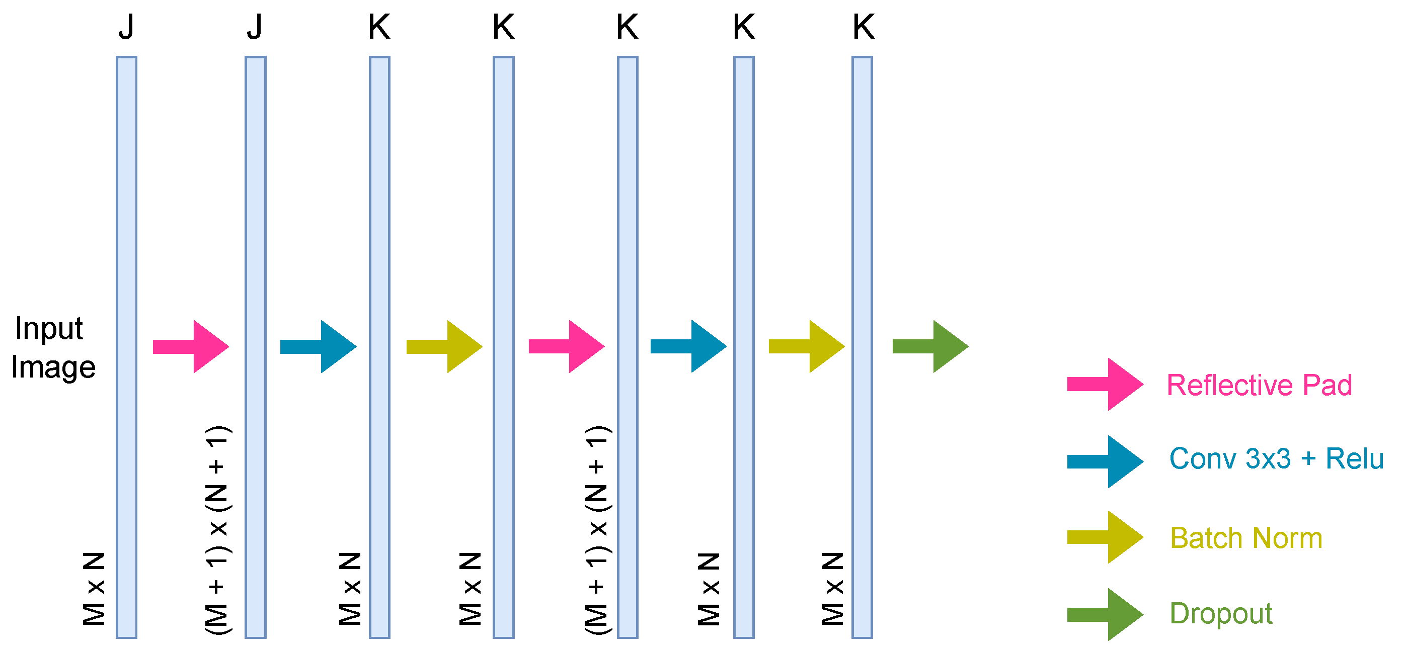
Figure 4 shows the modified convolution block used to construct our optimized network. At the end of each convolutional block, we added a dropout layer with a probability of 0.3. Dropout is a neural network regularization strategy employed to reduce interdependent learning between neurons, lowering the risk of network overfitting. Moreover, it forces the network to learn more robust features that can operate well in conjunction with distinct random subsets of other neurons. In addition to dropout, we inserted a batch normalization layer at the end of each convolutional layer to increase the stability of a neural network. Indeed, each layer input has a corresponding distribution during the training process affected by the parameter initialization and input data randomness. These randomnesses on the internal layer inputs distribution are described as internal covariate shift, and batch normalization is used to mitigate these effects [29]. Finally, we added a padding layer for each convolutional layer to keep the image size within the entire network unchanged. Indeed, the standard UNet does not perform any padding in the convolution layers, and the output size for each layer is not equal to the input size; in particular, we used a specific type of padding, i.e., reflecting padding, to preserve the physical structure of the SAR image both in terms of amplitude and interferometric phase values.

3.2. Network Structure

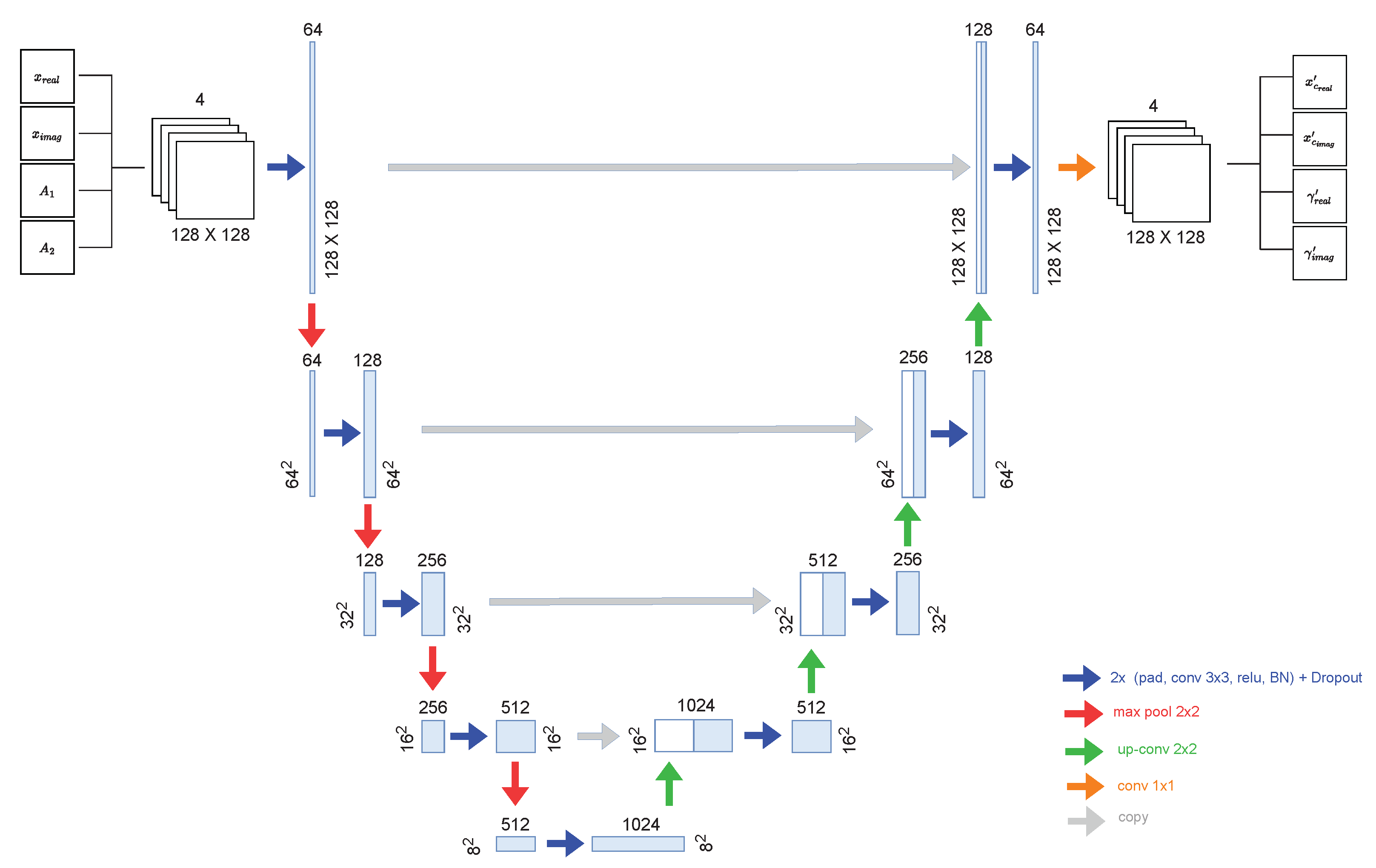
Figure 5 shows the architecture derived from the original U-Net. As explained above, the UNet architecture follows the structural composition of an encoder–decoder. Both the encoder, bottleneck and decoder are composed of our modified convolutional blocks, i.e., the ensemble of convolutional layer (Conv), batch normalization (BN), ReLU activation functions and dropout, as depicted in Figure 4. A two-by-two max-pooling follows each convolutional block in the encoder path. Note that the number of feature maps after each block doubles (from 64 to 1024) so that architecture can effectively learn complex structures. The bottleneck, composed of one convolutional block followed by a two-by-two upsampling transposed convolutional layer, mediates between the encoder and decoder layers. On the decoder side, a two-by-two upsampling transposed convolutional layer follows each convolutional block, and the number of decoder filters is halved (from 1024 to 64) to maintain symmetry during the corresponding reconstruction. After each transposed convolution, the image is concatenated with the corresponding one from the encoder through the skip connection. As explained above, skip connections help recover the information that may have been partially lost during the encoding phase, allowing for a more detailed reconstruction. Finally, the last decoder building block comprises a one-by-one convolution layer with a filters number equal to the number of the desired output, i.e., 4.

3.3. Learning

In order to extract accurate information from the filtered signal, phase unwrapping procedures must be performed to retrieve the absolute phase. Therefore, it is essential to preserve good phase detail features (e.g., fringes and edges) during the noise filtering to ensure measurement accuracy in the subsequent processing step. Note that the window size and shape used in most of the classical filtering methods are automatically set by the network during the learning process, and it is not visible outside the network. All the architectures present in the literature [18,19,20] are trained to address the filtering problem by learning the filtered interferometric phase (real and imaginary part) directly from their corresponding noise-free ground truth. However, this approach, typically used in the natural images field, cannot be used for interferometric phase filtering as it generates artefacts in the reconstructed signal. This behavior is due to the fact that some InSAR phase images are characterized by low-coherence (i.e., low SNR) or high-frequency fringes areas where the noise amount does not allow to retrieve the original signal. Consequently, developing a suitable training phase to preserve the original phase noise input into these crucial areas is necessary. More in detail, in the noisy areas, i.e., coherence close to zero, we preserve the original data as it is impossible to estimate any signal. On the other hand, in the high-coherence areas characterized by a low expected a posteriori variance, we filter out the noise to completely recover the underlying signal. Finally, in fast fringes and low-coherence areas, where a greater a posteriori variance is expected, we partially filter the noisy input signal to avoid introducing artefacts. Thus, the desired behavior is achieved by creating a “noisy” ground truth where the noise level depends on the expected estimate a posteriori variance as a function of the coherence and spatial frequency.

Starting from the simulated noiseless interferometric phase image ${\varphi }_c$, we computed the magnitude gradient $\nabla \left({\varphi }_c\right)$ using a 5 × 5 Sobel filter to extract phase fringes frequency information. We then created a specific function that manages the overlap between the pixels to be filtered and those in which the original noise must be kept. The overlap function $S2$, computed using a series of two $logistic$ functions that takes in the magnitude gradient $\nabla \left({\varphi }_c\right)$ and the coherence values $\rho$, respectively, is defined as

$$S2=\frac{1}{1+e^{-k(\rho -S1)}}$$

(25)

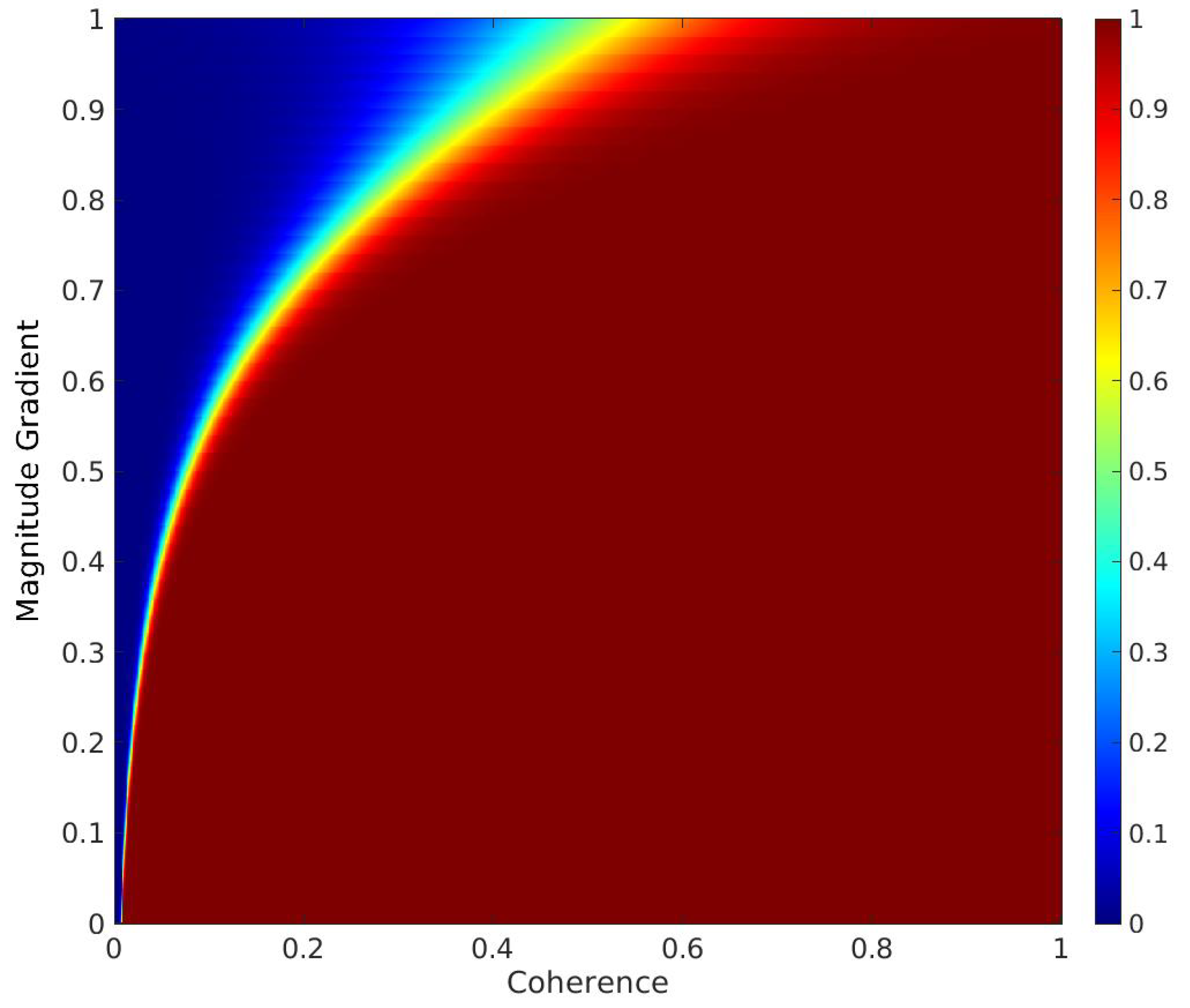
where

$$S1=\frac{b}{1+e^{-m(\nabla \left({\varphi }_c\right)-q)}}$$

(26)

and k is an exponential increasing factor associated to each magnitude gradient value range. The tuning parameters b, m and q, empirically set after preliminary experiments, are used to manage the overlap function and provide different filtering versions. Figure 6 shows an example of the overlap function $S2$ used during training.

Finally, for each pixel in the images, we first calculate the associated overlap values, and then we compute the “mixed” ground truth as

$${\varphi }_{mixed}=angle(S2·e^{(j*{\varphi }_c)}+(1-S2)·e^{(j*\varphi )})$$

(27)

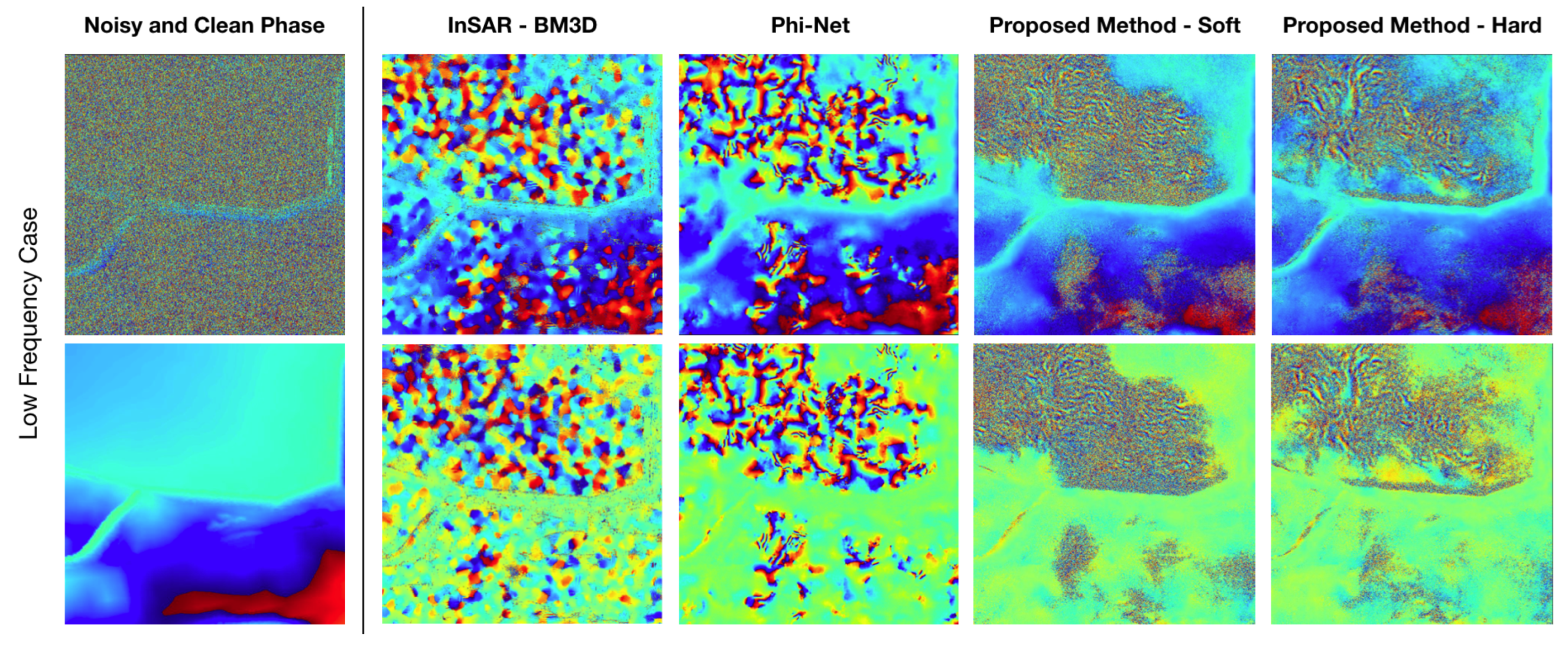
Figure 7 shows an example of a “mixed” ground truth based on magnitude gradients and the coherence values.

3.4. Loss Function

The loss function is essential during neural network training to update the network’s weights and build a better-fitting model. To optimize our network parameters, we exploit a combination of two Mean Square Error (MSE) by minimizing the error between the predicted image and the “mixed” ground truth as

$${\mathcal{L}}_{tot}={\mathcal{L}}_{phase}+\beta ·{\mathcal{L}}_{coh}$$

(28)

where the weight $\beta =7$ is empirically set to ensure that the losses rely on the same range of values. The first MSE, related to the phase prediction of the filtered real and imaginary part, is defined as

$${\mathcal{L}}_{phase}=\frac{1}{N}\sum _{i=1}^N(||x_i-x_i^{\prime }{||}_2^2)$$

(29)

with

$$x_i=[Re\left(e^{j·{\varphi }_{i_{mixed}}}\right),Im\left(e^{j·{\varphi }_{i_{mixed}}}\right)]$$

(30)

$$x_i^{\prime }=[Re\left(e^{j·{\varphi }_{i_{mixed}}^{\prime }}\right),Im\left(e^{j·{\varphi }_{i_{mixed}}^{\prime }}\right)]$$

(31)

where N is the number of pixels of the images, $x_i$ and $x_i^{\prime }$ represent the label and the network output of the $i_{th}$ pixel. On the other hand, the second MSE is related to the coherence estimation, and it is defined as

$${\mathcal{L}}_{coh}=\frac{1}{N}\sum _{i=1}^N(w_i||y_i-y_i^{\prime }{||}_2^2)$$

(32)

with

$$y=[Re(\rho ·e^{j·{\varphi }_{i_{mixed}}}),Im(\rho ·e^{j·{\varphi }_{i_{mixed}}})]$$

(33)

$$y^{\prime }=[Re(\rho ·e^{j·{\varphi }_{i_{mixed}}^{\prime }}),Im(\rho ·e^{j·{\varphi }_{i_{mixed}}^{\prime }})]$$

(34)

where N is the number of pixels of the images, $y_i$ and $y_i^{\prime }$ represent the label and the network output of the $i_{th}$ pixel and $w_i$ is the weight term applied to balance the loss function with respect to the coherence values of our dataset. The additional weight is calculated as

$$w_i=\sqrt{\frac{N_{tot}}{N_k}}\mathrm{with}k=1,2......70$$

(35)

where $N_{tot}$ is the dataset total number of pixels and $N_k$ is the number of pixels of the coherence interval k to which the considered $i_{th}$ pixel belongs. The coherence histogram is evaluated over 70 bins uniformly distributed. Note that the two loss functions are based on two different signal model that differ from each other by the coherence $\rho$ multiplicative term as depicted in Equations (31) and (33). The reason why we do not estimate the filtered phase ${\varphi }_{mixed}$ directly from the second model (i.e., $\rho ·e^{j·{\varphi }_{mixed}}$) lies in the fact that, in this way, the network is no longer able to estimate the noisy part of the “mixed” ground truth during training.

4. Results

We created an appropriate set of experiments that included synthetic and real images to evaluate our model performance. The synthetic dataset enables us to quantitatively compare the accuracy of our predictions to the other state-of-the-art (SOA) techniques, while real InSAR images are employed to show how the suggested architecture can be successfully applied in a real setting. All the experiments were performed with an NVIDIA RTX Ti 2080 GPU.

Table 1. Values of parameters used for network training.

Parameters Configuration
optimizer	AdamW
base learning rate	1 × 10${}^{-3}$
weight decay	0.01
amsgrad	False
optimizer momentum	${\beta }_1,{\beta }_2$ = 0.9, 0.999
batch size	64
training epochs	320
training time	3.20 h
gradient clip	1
precision	Mixed precision (16 bit)

summarizes the settings used for our main results. In the following section, we provide an overview of the dataset we created to conduct the experiments, and we show our results in comparison with the state-of-the-art methods together with the final conclusions that can be drawn.

4.1. Synthetic Dataset

Our semi-synthetic dataset has been built using the phase model and the simulated method described above. The dataset is composed of 128 × 128 patches extracted from four different mining sites. In particular, the training set contains 5400 patches extracted from three mining sites and the validation set contains 1900 patches extracted from another mining site. Both datasets are built to have a number of balanced patches in terms of the coherence and phase fringes values.

Table 2. Values of parameters used for the simulation of synthetic phase patterns.

Simulation Parameters
wavelength	6 cm
sensor-to-target distance	600 km
average local incidence angle	$\frac{\pi }{6}$ rad
baseline	100, 300, 600, 900, 1200, 1500 m

summarizes the parameters used to construct them. Note that the listed parameters identify a simulation strategy considering an acquisition through a point antenna (i.e., the infinite critical baseline). The spatial coherence losses caused by the baseline decorrelation are already included in the coherence estimation computed over the stack of images considered.

Each patch includes three channels that correspond to the parameters used to simulate the interferograms (i.e., A, $\rho$ and ${\varphi }_c$) according to Equations (2) and (3). In our setting, the simulation procedure is carried out online. In other words, new synthetic images are created for each training phase iteration. This type of approach allows the model to mitigate overfitting, thus avoiding losing generalization capabilities on unseen samples. Indeed, by introducing a distinct noise image at each training step, the model is driven to learn a more robust mapping between the input and label pairs. Additionally, the samples are augmented at each training step by randomly combining ${90}^{\circ }$ and ${270}^{\circ }$ rotations, horizontal and vertical flips and flipping in both directions.

4.2. Performance Evaluation

We compared the proposed method against the InSAR-BM3D [16], NL-InSAR [15], and Phi-Net methods [10] on both the simulated and real InSAR data. The evaluation of the final results was carried out using qualitative and quantitative criteria. In particular, the qualitative evaluation is based on visual observation. Therefore, we provide filtered and noisy interferometric phase images together. This evaluation method checks whether the noise is reduced, the phase fringes are maintained and artefacts are not introduced. On the other hand, the quantitative indexes are based on the Mean Square Error (MSE) and the Spectral Flatness (SF) between the filtered and ideal phases. The MSE metric measures the difference between the filtered and clean interferometric phases. Smaller values correspond to the filtered interferometric phase closer to the clean one. However, this index does not consider the artefacts introduced where the original signal cannot be filtered due to a large amount of noise. This is critical as, in many InSAR processing applications (e.g., motion displacement monitoring), data artefacts lead to an erroneous analysis with consequent unreliable results. Therefore, it is better to sacrifice complete filtering to reduce the chance of having fringe artefacts in the reconstructed signal. To solve this problem, we adopt a spectral-flatness index which consists of a flatness evaluation of the residue spectrum. The residues are defined as the difference between filtered and clean interferometric phases. This custom metric indicates the number of uncontrolled artefacts introduced during the filtering process. When the flatness of the spectrum is low, the residual spectral power is concentrated in a limited number of bands, and consequently, a large amount of uncontrolled artefacts is present in the predicted image. Instead, high values of spectral flatness indicate that the spectrum has roughly equal power throughout all spectral bands, making the spectrum graph appear smooth and flat. Figure 8 shows a comparison example between a low- and high-spectral-flatness case. The final filtering evaluation is computed simultaneously, considering the MSE and spectral flatness as filtering and artefacts indicators. In particular, in order to balance the metrics and validate the results, we adopt a combination of the MSE and SF, defined as

$$\frac{MSE}{\sqrt{SF}}$$

(36)

The coherence estimation performance is computed instead, considering only the MSE between the prediction and the ground truth.

4.3. Experiments on Simulated Data

Visual comparisons with the considered coherence and filtering estimation methods are presented. In particular, for the filtering part, we compared our result with respect to InSAR-BM3D and Phi-Net as classical and deep learning-based SOA methods, respectively. On the other hand, because InSAR-BM3D does not estimate the coherence, we compared our coherence predictions with respect to NL-InSAR and Phi-Net. In order to better understand how our network manages the critical area in which the original signal cannot be restored, we provide two filtering versions obtained by tuning the parameters b, m and q in Equation (26). More in detail, the soft version (m = 5, q = 0.78 and b = 0.85) generates fewer artefacts, maintaining the original input noise. Opposite to that, the hard version (m = 5, q = 1 and b = 1) tries to filter as much as possible, thus generating some artefacts in the final prediction. In addition to the predicted images, we also show the residual phase map corresponding to the difference between the estimated quantity and its corresponding clean reference. We consider three different case studies depending on the phase fringe frequency (i.e., low, medium and high).

From the first visual inspection in Figure 9, Figure 10 and Figure 11, it is visible that the proposed architecture outperforms all previous SOA approaches in all the considered cases as it can accurately reconstruct details even with strong noise levels. Our model is more effective than other techniques in separating the noise contribution from the underlying informative signal. Indeed, we can follow the fringes structures even in interruptions due to a large amount of noise present in the image. Furthermore, it is possible to observe how the model does not introduce large artefacts, thus making the prediction usable for a subsequent phase unwrapping step. As shown in Figure 12, also in the coherence estimation, it is visible that the proposed method can maintain a significantly higher level of detail than the SOA ones. The numerical results, summarized in Figure 13, Figure 14 and Figure 15, confirm that the proposed model significantly outperforms all other methods on the most coherence bins for the custom combined metric (Equation (36)) considered. Note that, although the MSE for some bins is similar in the filtering prediction, the spectral-flatness values differ significantly. This behavior emphasizes that the MSE is not always a good indicator of the filtering performance. Indeed, the introduction of noise in the prediction sometimes implies a worsening of the comparison with the ground truth, but on the other hand, it is responsible for a notable increase in the spectral flatness (i.e., it does not generate artefacts). In contrast to that, completely different behavior for the InSAR-BM3D method can be noticed. Here, the spectral flatness assumes high values despite the high values of the MSE. This trend is due to the wrong noise content in the filtered interferograms, which, on one side, causes an increase in the MSE and, on the other side, makes the spectrum smooth and causes an increase in the spectral flatness. The custom combined metric provides a complete evaluation of the filtering performance for all the possible behaviors.

Table 3. Quantitative index Equation (36) of the compared methods on simulated low-frequency fringes.

Low Frequency
Coherence Range	Methods
	InSAR- BM3D	Phi-Net	Soft	Hard
0–0.3	1.9190	2.0199	2.1121	1.7909
0.3–0.6	0.6940	0.2448	0.1865	0.1602
0.6–1	0.3502	0.0927	0.0478	0.0456

,

Table 4. Quantitative index Equation (36) of the compared methods on simulated medium-frequency fringes.

Medium Frequency
Coherence Range	Methods
	InSAR- BM3D	Phi-Net	Soft	Hard
0–0.3	3.4832	3.4673	2.6974	2.5543
0.3–0.6	1.3924	0.7199	0.4749	0.3977
0.6–1	0.6577	0.2181	0.0822	0.0799

and

Table 5. Quantitative index Equation (36) of the compared methods on simulated high-frequency fringes.

High Frequency
Coherence Range	Methods
	InSAR- BM3D	Phi-Net	Soft	Hard
0–0.3	3.6572	4.1706	3.1042	3.0426
0.3–0.6	2.4025	1.4076	1.0314	0.8700
0.6–1	2.1257	0.4811	0.2466	0.2015

show the final numerical result of the combined metric considering the three different phase fringe frequency cases separately. Finally,

Table 6. Mean square error of the compared methods on simulated coherence data.

Coherence Range	Methods
	NL-InSAR	Phi-Net	Proposed Method
0–0.3	0.0060	0.0025	0.0024
0.3–0.6	0.0622	0.0700	0.0525
0.6–1	0.0959	0.0949	0.0601

and Figure 16 confirm that the proposed method can also maintain a significantly higher level of detail in the coherence estimation, outperforming the other ones.

4.4. Experiment on Real Data

This section provides the results from real interferometric SAR images acquired by the TerraSAR-X and the Sentinel-1 missions. We tested our proposed method on areas where the water presence guarantees fixed low-coherence values with consequent noisy phase areas. In particular, for the TerraSAR-X example, we selected a scenario related to an acquisition of the Miami coast overlooking the Atlantic Ocean. The choice of this place lies in the fact that, as shown in Figure 17 (site A-I), we want to test our methodology in water areas characterized by different amplitude values. In this way, we ensure that the coherence predictions are not strictly linked to the value of the amplitude input, and consequently, the network keeps the phase noise correctly as the final prediction. As shown in Figure 17 (site A-II), we also tested our method in mountainous areas, where the presence of geometric distortions, such as layover, foreshortening and shadows, causes spatial decoration with a consequent loss of coherence. Finally, concerning the Sentinel-1 images in Figure 17 (site A-III), we use the exact test images presented in the Phi-Net paper to directly compare the two deep learning-based methods.

We employ a qualitative comparison to assess the filtering performance rather than a quantitative evaluation as we do not have noise-free real images to compute the metrics. As can be noticed from Figure 18, the proposed method has powerful denoising abilities on real InSAR data. Contrary to other methods, we can observe that we provide a strong noise suppression, keeping the noise input in the areas where the original signal cannot be filtered. Indeed, it is possible to highlight how the artefacts in the incoherent noisy area are significantly reduced, and the filtered dense interferometric fringe patterns appear cleaner and smoother. Note that the soft version provides a more conservative filtering estimation that can be used to obtain a completely reliable phase unwrapping final result. As shown in Figure 19, a similar result is observed for the coherence as well. Indeed, our network estimates appear more detailed than the NL-InSAR and Phi-Net ones.

Moreover, it can be noted that the coherence values relating to the water areas are much lower in our prediction than the others. The greater precision in the estimation is due to the fact that our network, unlike other works in the literature, has been trained with simulated data starting from real data. This allowed us to replicate physical behaviors typical of InSAR data, providing reliable images. Similar results can be observed in the Sentinel-1 data, as shown in Figure 20 and Figure 21. According to the results obtained from the TerraSAR-X data, we note that we can suppress the noise and preserve details in both the phase and the coherence images. As before, the soft version provides a conservative estimate of the filtering, thus ensuring a completely reliable result.

5. Discussion

In this article, we presented a novel deep learning model to estimate both the coherence and the interferometric phase from SAR data. In particular, we designed a learning strategy that, combined with a novel data simulation procedure, allowed us to train a CNN architecture suitable for interferometric phase processing. The first contribution is based on integrating a novel learning paradigm into network training. The methodology implemented, which has never been explored before for the InSAR filtering task, has shown interesting features. The desired behavior, achieved by creating a ground truth containing noise pixels where the original signal cannot be filtered, effectively represents the interferometric signal and the superimposed noise. It results in our network’s ability to maintain any fringe density patterns while keeping the original noise in the critical areas. A visual examination of the synthetic data phase and coherence images demonstrates that the phase fringe structures are well-preserved compared to the other SOA methods. In this way, thanks to the a priori knowledge on the wrap count, we can guarantee a completely reliable filtering result than can be used in the subsequent phase unwrapping step. Furthermore, real InSAR data experiments confirm our observations made on the synthetic data. Indeed, we can preserve high-resolution details and spatial textures while maintaining the original noisy input in areas where the underlying signal cannot be reconstructed. The training dataset plays a key role in the performance estimation. Our data generation has been realized, starting from real InSAR acquisitions. In this way, the physical behaviors typical of real InSAR data are considered to model the relationships between the amplitude, coherence and interferometric phase. The addition of these valuable details greatly enhanced the network performance. Indeed, the model can outperform the SOA approaches on the examined test cases composed of synthetic test patterns and real data. In future developments, we plan to compare different phase unwrapping methods using the proposed filtering results as input.