


Estimation of Chlorophyll-A Concentration with Remotely Sensed Data for the Nine Plateau Lakes in Yunnan Province
 ,
,  , ,
, ,  , , and
Abstract
1. Introduction
2. Materials
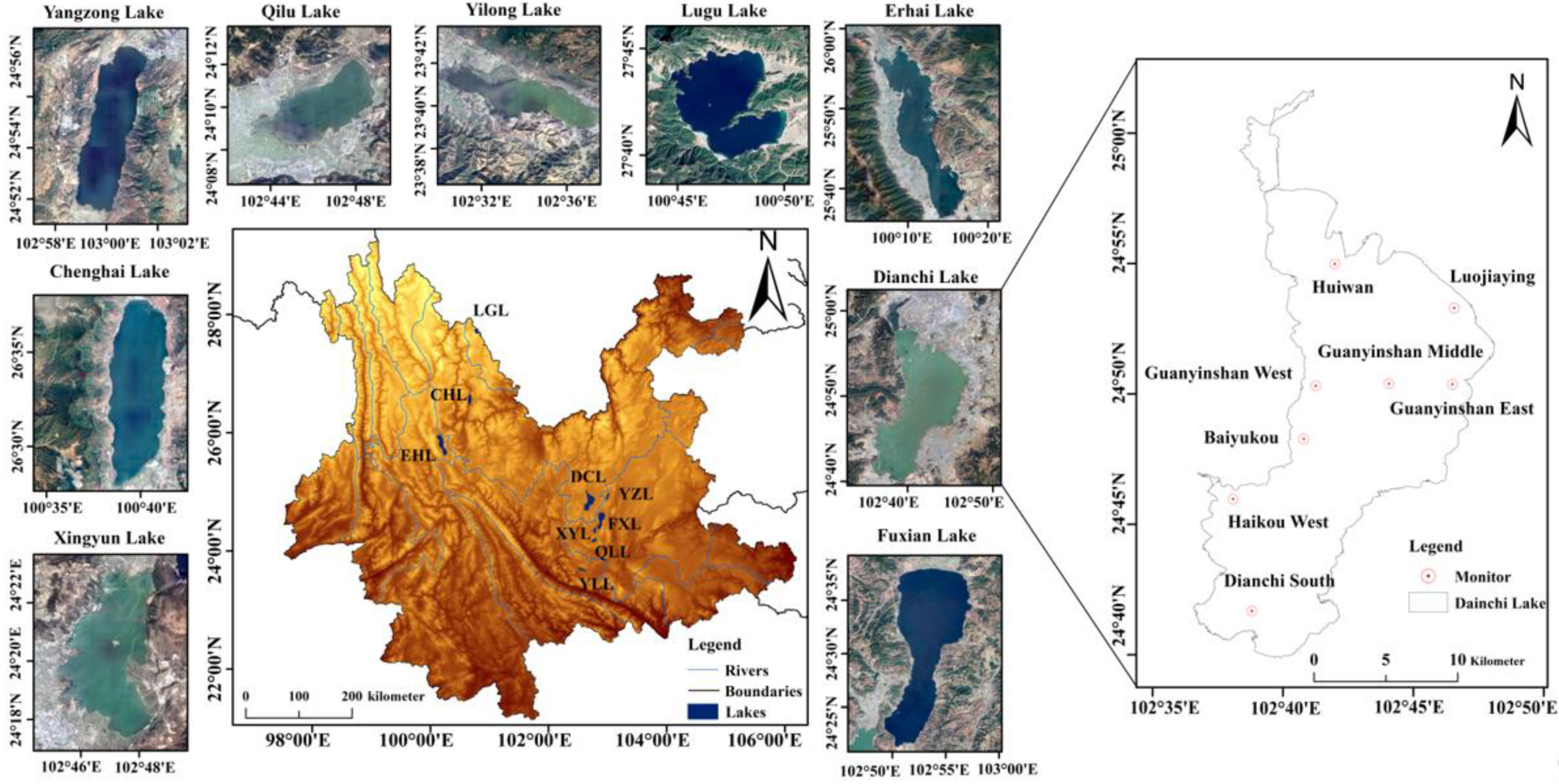
2.1. Study Area
2.2. Data
3. Methods
3.1. Water Body Extraction
3.2. Retrieval Model Construction of the CCAPL
3.3. RF Algorithm Feature Selection
3.4. CCAPL Retrieval and Evaluation Methods
3.5. Lake Surface Temperature Retrieval
4. Results
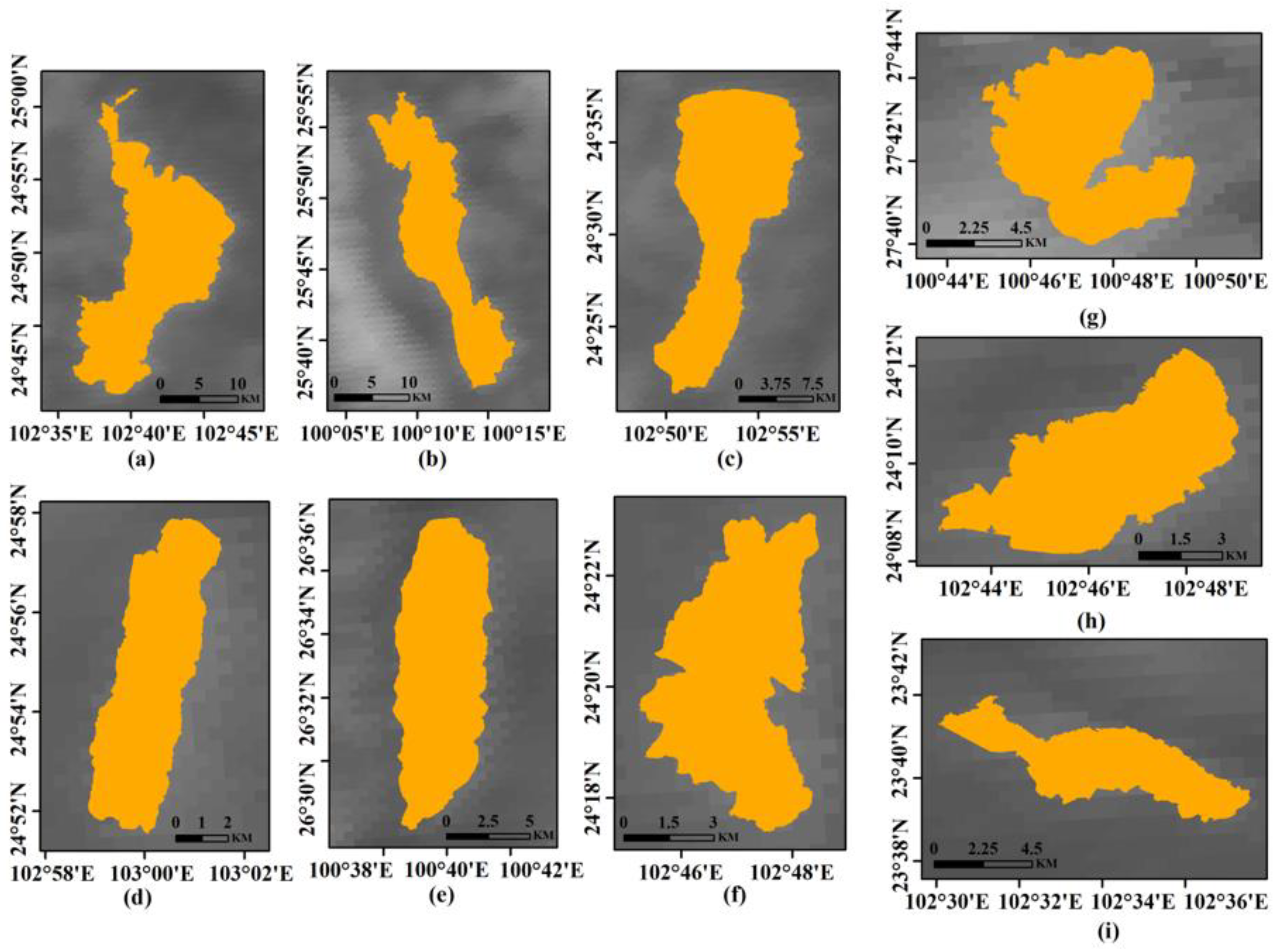
4.1. Extraction Results of Water Bodies
4.2. CCAPL Model and Accuracy Evaluation
4.3. Retrieval of the CCAPL
4.4. Retrieval of the STPL
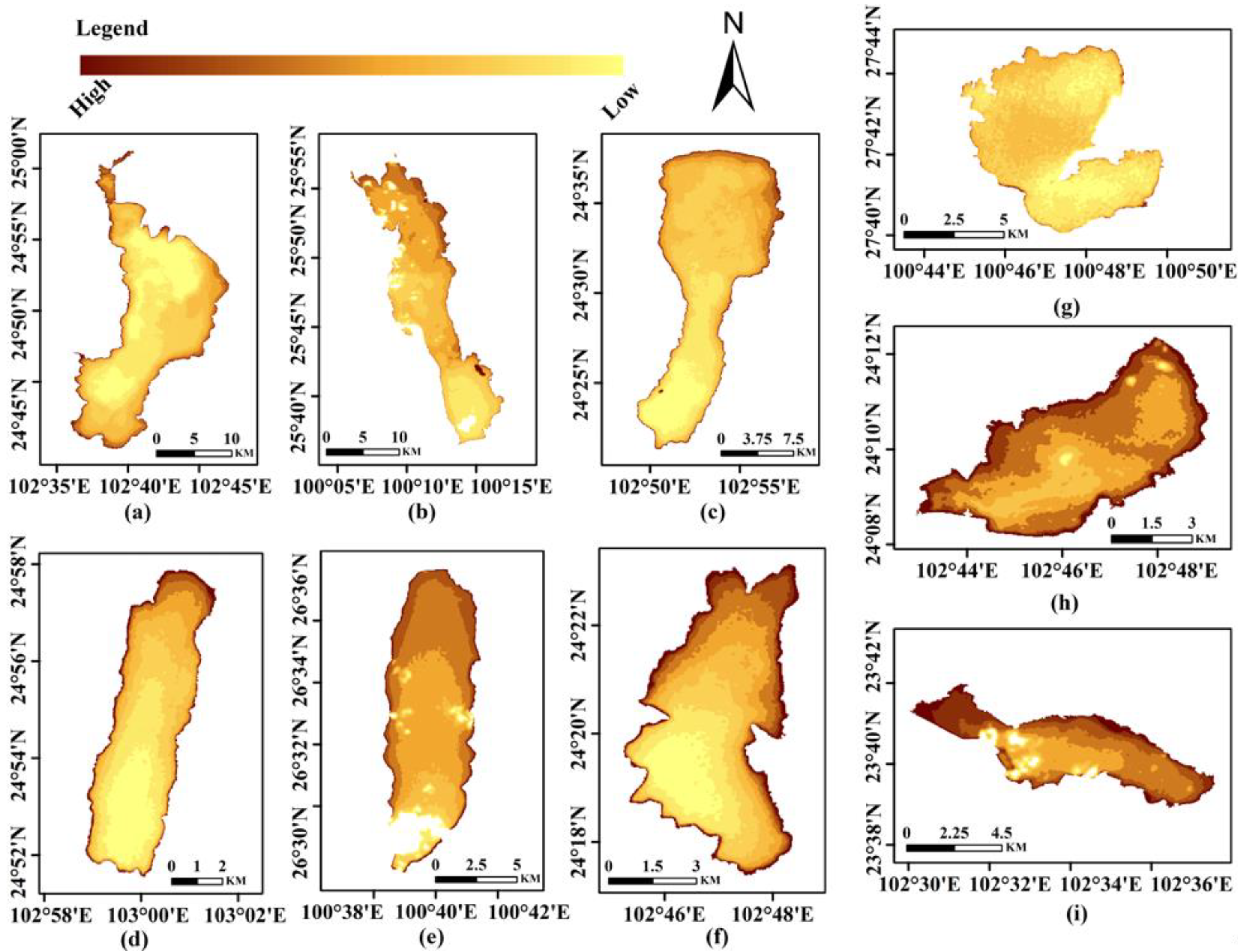
4.5. Spatial Correlation Analysis
5. Discussion
6. Conclusions
- (1)
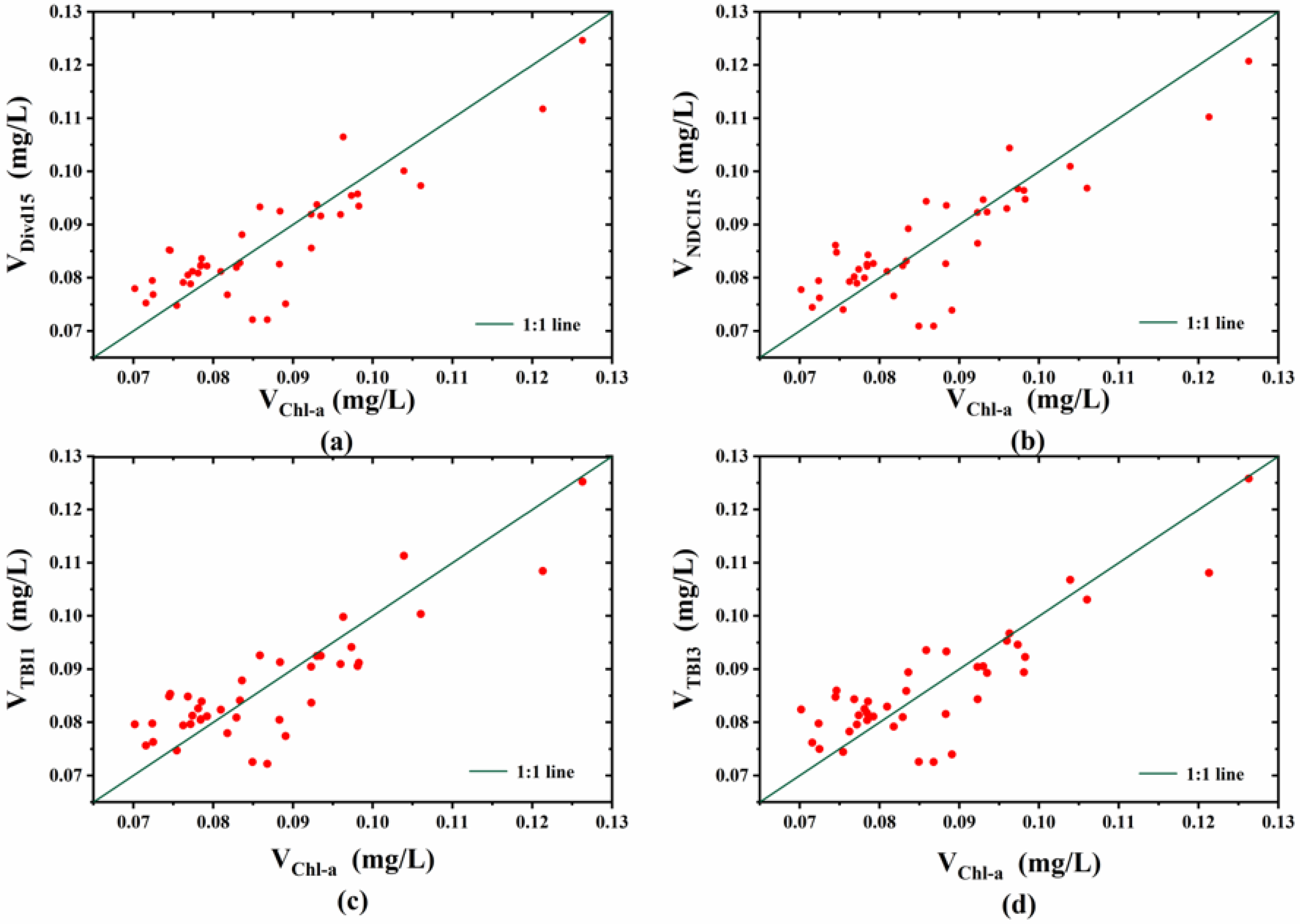
- According to the ranked RF feature importance, the spectral indexes that strongly correlated with the chlorophyll-a concentration were selected for the CCAPL retrieval. We analyzed the relative error and accuracy. Among the four models, NDCI15 had the best accuracy, with an RMSE of 0.0249, an MAE of 0.0142 and a MAPE of 26.30%.
- (2)
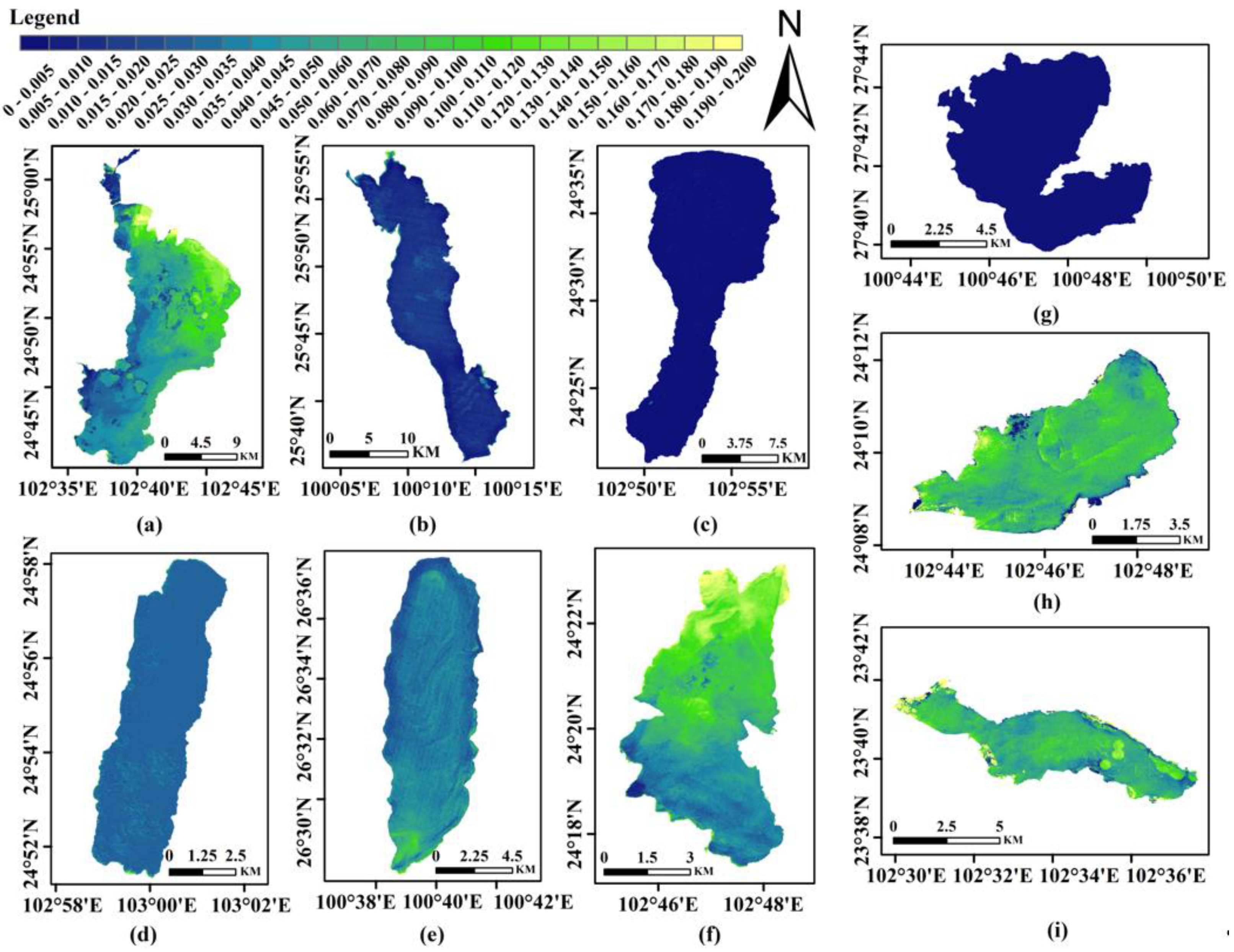
- The lakes with chlorophyll-a concentrations of less than 0.03 mg/L were Chenghai Lake, Yangzong Lake, Erhai Lake, Fuxian Lake and Lugu Lake, among which the chlorophyll-a concentrations of Erhai Lake, Fuxian Lake and Lugu Lake were less than 0.01 mg/L. The lakes with chlorophyll-a concentrations between 0.03 and 0.1 mg/L were Dianchi Lake and Xingyun Lake. The average value of the chlorophyll-a concentration in the northeast of Dianchi Lake and the north of Xingyun Lake was 0.085 mg/L. The lakes with chlorophyll-a concentrations greater than 0.1 mg/L were Yilong Lake and Qilu Lake, among which the chlorophyll-a concentration in Qilu Lake was greater than 0.14 mg/L.
- (3)
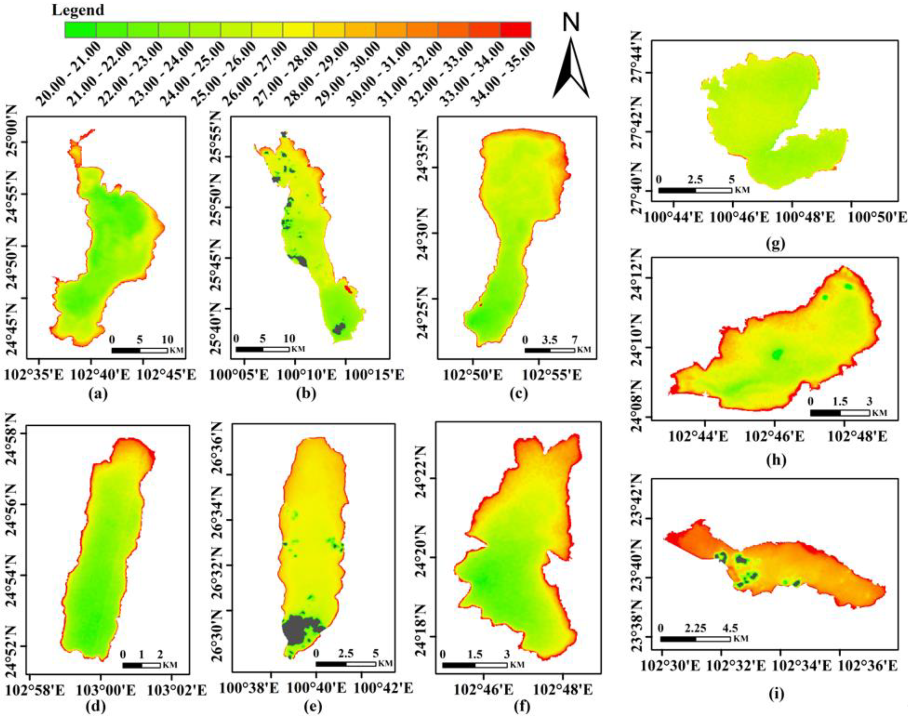
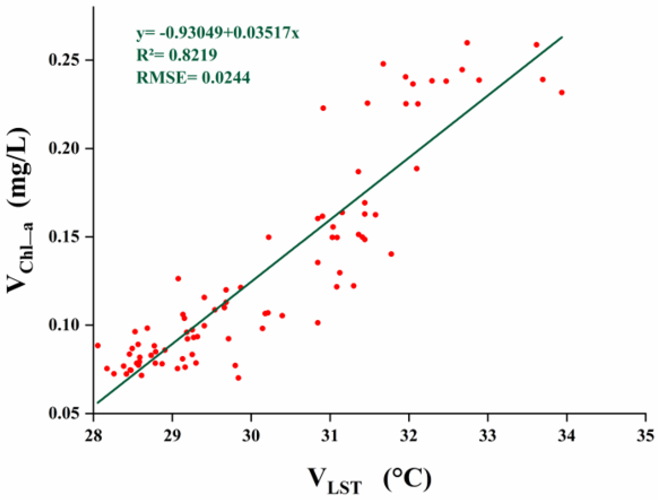
- When the STPL was within 28–34 °C, it had an obvious correlation with the chlorophyll-a concentration, and the correlation increased gradually from the lakes’ center to the shore. When the lakes’ temperatures rise, this provides a key monitoring area for managers. Considering the relatively limited surface monitoring data, the next plan is to accumulate more surface experimental data for the plateau lakes, conduct seasonal analysis or add other hydrological factors to explore the coupling mechanism of the CCAPL and other impurities in the water.
Author Contributions
Funding
Data Availability Statement
Acknowledgments
Conflicts of Interest
References
- Zhang, Y.; Ma, R.; Liang, Q.; Guan, B.; Loiselle, S. Secondary impacts of eutrophication control activities in shallow lakes: Lessons from aquatic macrophyte dynamics in Lake Taihu from 2000 to 2015. Freshw. Sci. 2019, 38, 802–817. [Google Scholar] [CrossRef]
- An, Y.; Kampbell, D. Monitoring Chlorophyll- a as a Measure of Algae in Lake Texoma Marinas. Bull. Environ. Contam. Toxicol. 2003, 70, 606–611. [Google Scholar] [CrossRef]
- Caballero, I.; Navarro, G. Monitoring cyanoHABs and water quality in Laguna Lake (Philippines) with Sentinel-2 satellites during the 2020 Pacific typhoon season. Sci. Total. Environ. 2021, 788, 147700–147712. [Google Scholar] [CrossRef]
- Palmer, S.; Kutser, T.; Hunter, P. Remote sensing of inland waters: Challenges, progress and future directions. Remote Sens. Environ. 2014, 157, 1–8. [Google Scholar] [CrossRef]
- Xu, J.; Gao, C.; Wang, Y. Extraction of spatial and temporal patterns of concentrations of chlorophyll-a and total suspended matter in poyang lake using GF-1 satellite data. Remote Sens. 2020, 12, 622. [Google Scholar] [CrossRef]
- Tilstone, G.; Pardo, S.; Dall’Olmo, G.; Brewin, R.; Nencioli, F.; Dessailly, D.; Kwiatkowska, E.; Casal, T.; Donlon, C. Performance of Ocean Colour Chlorophyll a algorithms for Sentinel-3 OLCI, MODIS-Aqua and Suomi-VIIRS in open-ocean waters of the Atlantic. Remote Sens. Environ. 2021, 260, 112444. [Google Scholar] [CrossRef]
- Mark, A.; Stefan, G.; Nick, S. Complementary water quality observations from high and medium resolution Sentinel sensors by aligning chlorophyll-a and turbidity algorithms. Remote Sens. Environ. 2021, 265, 112651. [Google Scholar]
- Pahlevan, N.; Smith, B.; Binding, C.; Gurlin, D.; Li, L.; Bresciani, M.; Giardino, C. Hyperspectral retrievals of phytoplankton absorption and chlorophyll-a in inland and nearshore coastal waters. Remote Sens. Environ. 2021, 253, 112200. [Google Scholar] [CrossRef]
- Wu, H.; Liao, M.; Guo, J.; Zhang, Y.; Liu, Q.; Li, Y. Diatom assemblage responses to multiple environmental stressors in a deep brackish plateau lake, SW China. Environ. Sci. Pollut. Res. Int. 2022, 29, 33117–33129. [Google Scholar] [CrossRef] [PubMed]
- Luo, J.; Qin, L.; Mao, P.; Xiong, Y.; Zhao, W.; Gao, H.; Qiu, G. Research Progress in the Retrieval Algorithms for Chlorophyll-a, a Key Element of Water Quality Monitoring by Remote Sensing. Int. Remote Sens. 2021, 36, 473–488. [Google Scholar]
- Sagan, V.; Peterson, K.; Maimaitijiang, M.; Sidike, P.; Sloan, J.; Greeling, B.; Maalouf, S.; Adamset, C. Monitoring inland water quality using remote sensing: Potential and limitations of spectral indices, bio-optical simulations, machine learning, and cloud computing. Earth-Sci. Rev. 2020, 205, 103187. [Google Scholar] [CrossRef]
- Liu, C.; Zhu, L.; Li, J.; Wang, J.; Ju, J.; Qiao, B.; Ma, Q.; Wang, S. The increasing water clarity of Tibetan lakes over last 20 years according to MODIS data. Remote Sens. Environ. 2021, 253, 112199. [Google Scholar] [CrossRef]
- Seegers, B.; Werdell, P.; Vandermeulen, R.; Salls, W.; Stumpf, R.; Schaeffer, B.; Owens, T.; Bailey, S.; Scott, J.; Loftin, K. Satellites for long-term monitoring of inland U.S. lakes: The MERIS time series and application for chlorophyll-a. Remote Sens. Environ. 2021, 266, 112685. [Google Scholar] [CrossRef]
- Xu, Y.; Dong, X.; Wang, J. Use of Remote Multispectral Imaging to Monitor Chlorophyll-a in Taihu Lake: A Comparison of Four Machine Learning Model. J. Hydroecol 2019, 40, 48–57. [Google Scholar]
- Zhang, Q.; Wu, Z. Research progress of the inversion algorithm of chlorophyll-a concentration in estuaries and coastal waters. Ecol. Sci. 2017, 36, 215–222. [Google Scholar]
- Wang, H.; Yang, F.; Luo, Z. An experimental study of the intrinsic stability of random forest variable importance measures. BMC Bioinform. 2016, 17, 60–78. [Google Scholar] [CrossRef] [PubMed]
- Wu, Z.; Li, J.; Wang, R.; Shi, L.; Miao, S.; Lv, H.; Li, Y. Estimation of CDOM concentration in inland lake based on random forest using Sentinel-3A OLCI. J. Environ. Sci. 2018, 30, 979–991. [Google Scholar]
- Hang, X.; Li, Y.; Li, X.; Xu, M.; Sun, L. Estimation of Chlorophyll-a Concentration in Lake Taihu from Gaofen-1 Wide-Field-of-View Data through a Machine Learning Trained Algorithm. J. Meteorol. Res. 2022, 36, 208–226. [Google Scholar] [CrossRef]
- Xu, H. Retrieval of the reflectance and land surface temperature of the newly-launched Landsat 8 satellite. Chinese J. Geophys. 2015, 58, 741–747. [Google Scholar]
- Duan, S.; Ru, C.; Li, Z.; Wang, M.; Xu, H.; Li, H.; Wu, P.; Zhan, W.; Zhou, J.; Zhao, W.; et al. Reviews of methods for land surface temperature retrieval from Landsat thermal infrared data. Natl. Remote Sens. Bull. 2021, 25, 1591–1617. [Google Scholar]
- Holm-Hansen, O.; Lorenzen, C.; Holmes, R.; Strickland, J. Fluorometric Determination of Chlorophyll. J. Cons. Int. Explor. Mer. 1965, 30, 3–15. [Google Scholar] [CrossRef]
- Rahmat, A.; Daruati, D.; Ramadhani, W.; Ratnawati, H. Analysis of Normalized Different Wetness Index (NDWI) Using Landsat Imagery in the Ciletuh Geopark Area as Ecosystem Monitoring. IOP Conf. Ser. Earth Environ. Sci. 2022, 1062, 012037. [Google Scholar] [CrossRef]
- Xu, H. A Study on Information Extraction of Water Body with the Modified Normalized Difference Water Index (MNDWI). J. Remote Sens. 2005, 09, 589–595. [Google Scholar]
- Gordon, H.R.; Morel, A. Remote Assessment of Ocean Color for Interpretation of Satellite Visible Imagery: A Review; Springer: New York, NY, USA, 1983; Volume 37, p. 292. [Google Scholar]
- Liu, X.; Steele, C.; Simis, S.; Warren, M.; Tyler, A.; Spyrakos, E.; Selmes, N.; Hunter, P. Retrieval of Chlorophyll-a concentration and associated product uncertainty in optically diverse lakes and reservoirs. Remote Sens. Environ. 2021, 267, 112710. [Google Scholar] [CrossRef]
- Dekker, A.; Peters, S. The Use of the Thematic Mapper for the Analysis of Eutrophic Lakes: A Case Study in The Netherlands. Int. J. Remote Sens. 1993, 14, 799–822. [Google Scholar] [CrossRef]
- Lu, L.; Gong, Z.; Liang, Y.; Liang, S. Retrieval of Chlorophyll-a Concentrations of Class II Water Bodies of Inland Lakes and Reservoirs Based on ZY1-02D Satellite Hyperspectral Data. Remote Sens. 2022, 14, 1842. [Google Scholar] [CrossRef]
- Shi, H.; Li, X.; Niu, Z.; Li, J.; Li, Y.; Li, N. Remote sensing information extraction of aquatic vegetation in Lake Taihu based on Random Forest Model. J. Lake Sci. 2016, 28, 635–644. [Google Scholar]
- Ananias, P.; Negri, R.; Dias, M.; Silva, E.; Casaca, W. A Fully Unsupervised Machine Learning Framework for Algal Bloom Forecasting in Inland Waters Using MODIS Time Series and Climatic Products. Remote Sens. 2022, 14, 4283. [Google Scholar] [CrossRef]
- Goldstein, B.; Polley, E.; Briggs, F. Random Forests for Genetic Association Studies. Stat. Appl. Genet. Mol. Biol. 2011, 10, 32. [Google Scholar] [CrossRef]
- Minnett, P. Radiometric measurements of the sea-surface skin temperature: The competing roles of the diurnal thermocline and the cool skin. Int. J. Remote Sens. 2003, 24, 5033–5047. [Google Scholar] [CrossRef]
- Pyle, J. Planck’s radiation law: Spectral distribution and the gamma functions. J. Chem. Educ. 1985, 62, 488. [Google Scholar] [CrossRef]
- Qin, Z.; Li, W.; Xu, B.; Zhang, W. Estimation method of land surface emissivity for retrieving land surface temperature from Landsat TM6 data. Adv. Mar. Sci. 2004, 22, 129–137. [Google Scholar]
- Duan, S.; Li, Z.; Wang, C.; Zhang, S.; Tang, B.; Leng, P.; Gao, M. Land-surface temperature retrieval from Landsat 8 single-channel thermal infrared data in combination with NCEP reanalysis data and ASTER GED product. Int. J. Remote Sens. 2019, 40, 1763–1778. [Google Scholar] [CrossRef]
- Burnett, A.; Kirby, M.; Mullins, H.; Patterson, W. Increasing Great Lake-Effect Snowfall during the Twentieth Century: A Regional Response to Global Warming? J. Clim. 2003, 16, 3535–3542. [Google Scholar] [CrossRef]


| Bands | Name | Wavelength (nm) | Resolution (m) |
|---|---|---|---|
| Band 1 | Coastal | 0.433–0.453 | 30 |
| Band 2 | Blue | 0.450–0.515 | 30 |
| Band 3 | Green | 0.525–0.600 | 30 |
| Band 4 | Red | 0.630–0.680 | 30 |
| Band 5 | NIR | 0.845–0.885 | 30 |
| Band 6 | SWIR 1 | 1.560–1.660 | 30 |
| Band 7 | SWIR 2 | 2.100–2.300 | 30 |
| Band 8 | Pan | 0.500–0.680 | 15 |
| Band 9 | Cirrus | 1.360–1.390 | 30 |
| Band 10 | TIRS 1 | 10.60–11.19 | 100 |
| Band 11 | TIRS 2 | 11.50–12.51 | 100 |
| Bands | Name | Wavelength (nm) | Resolution (m) |
|---|---|---|---|
| Band 1 | Coastal aerosol | 0.433–0.453 | 60 |
| Band 2 | Blue | 0.458–0.523 | 10 |
| Band 3 | Green | 0.543–0.578 | 10 |
| Band 4 | Red | 0.650–0.680 | 10 |
| Band 5 | Vegetation red edge 1 | 0.698–0.713 | 20 |
| Band 6 | Vegetation red edge 2 | 0.733–0.748 | 20 |
| Band 7 | Vegetation red edge 3 | 0.773–0.793 | 20 |
| Band 8 | NIR | 0.785–0.900 | 10 |
| Band 8A | Vegetation red edge 4 | 0.935–0.955 | 20 |
| Band 9 | Water vapor | 1.360–1.390 | 60 |
| Band 11 | SWIR 1 | 1.565–1.655 | 20 |
| Band 12 | SWIR 2 | 2.100–2.280 | 20 |
| Name | Monitoring Time | * Number of Sampling Points |
|---|---|---|
| Dianchi Lake | 20200623 | 40 |
| Fuxian Lake | 20200622 | 30 |
| Chenghai Lake | 20200701 | 19 |
| Erhai Lake | 20200625 | 17 |
| Lugu Lake | 20200618 | 25 |
| Qilu Lake | 20200629 | 14 |
| Xingyun Lake | 20200627 | 17 |
| Yangzong Lake | 20200712 | 16 |
| Yilong Lake | 20200625 | 15 |
| ID | Band | Index Model | Feature Importance |
|---|---|---|---|
| 1 | B2 | B2 | 44.3066 |
| 2 | B3 | B3 | 43.9564 |
| 3 | B4 | B4 | 42.2547 |
| 4 | B5 | B5 | 43.6587 |
| 5 | B6 | B6 | 46.0333 |
| 6 | B7 | B7 | 45.0136 |
| 7 | B8 | B8 | 43.8657 |
| 8 | B8A | B8A | 39.3531 |
| 9 | B8/B4 | Divd1 | 35.9668 |
| 10 | B8/B5 | Divd2 | 37.7500 |
| 11 | B8/B6 | Divd3 | 46.0961 |
| 12 | B8/B7 | Divd4 | 38.5882 |
| 13 | B8/B8A | Divd5 | 47.3490 |
| 14 | B8A/B4 | Divd6 | 36.2064 |
| 15 | B8A/B5 | Divd7 | 40.1768 |
| 16 | B8A/B6 | Divd8 | 44.6549 |
| 17 | B8A/B7 | Divd9 | 41.3910 |
| 18 | B7/B4 | Divd10 | 38.5530 |
| 19 | B7/B5 | Divd11 | 44.2034 |
| 20 | B7/B6 | Divd12 | 45.7065 |
| 21 | B6/B5 | Divd13 | 49.2723 |
| 22 | B6/B4 | Divd14 | 44.8093 |
| 23 | B5/B4 | Divd15 | 49.4467 |
| 24 | B8 − B4/B8 + B4 | NDCI1 | 37.6184 |
| 25 | B8 − B5/B8 + B5 | NDCI2 | 44.9984 |
| 26 | B8 − B6/B8 + B6 | NDCI3 | 46.9481 |
| 27 | B8 − B7/B8 + B7 | NDCI4 | 39.0772 |
| 28 | B8 − B8A/B8 + B8A | NDCI5 | 46.5039 |
| 29 | B8A − B4/B8A + B4 | NDCI6 | 42.8151 |
| 30 | B8A − B5/B8A + B5 | NDCI7 | 43.4148 |
| 31 | B8A − B6/B8A + B6 | NDCI8 | 45.4098 |
| 32 | B8A − B7/B8A + B7 | NDCI9 | 48.7971 |
| 33 | B7 − B4/B7 + B4 | NDCI10 | 40.1548 |
| 34 | B7 − B5/B7 + B5 | NDCI11 | 40.1852 |
| 35 | B7 − B6/B7 + B6 | NDCI12 | 44.5754 |
| 36 | B6 − B5/B6 + B5 | NDCI13 | 41.0464 |
| 37 | B6 − B4/B6 + B4 | NDCI14 | 43.2968 |
| 38 | B5 − B4/B5 + B4 | NDCI15 | 56.2430 |
| 39 | (1/B4 − 1/B5)·B6 | TBI1 | 54.1088 |
| 40 | (1/B4 − 1/B5)·B7 | TBI2 | 44.7620 |
| 41 | (1/B4 − 1/B5)·B8 | TBI3 | 55.2735 |
| 42 | (1/B4 − 1/B5)·B8A | TBI4 | 42.9489 |
| Name | Model | Linear Fitting | R-Squared |
|---|---|---|---|
| Dianchi Lake | NDCI15 | y = 0.0347 + 0.2832x | 0.7246 |
| Divd15 | y = −0.0408 + 0.0873x | 0.7467 | |
| TBI1 | y = 0.0466 + 0.1435x | 0.7298 | |
| TBI3 | y = 0.0453 + 0.1715x | 0.7164 | |
| Erhai Lake | NDCI15 | y = 0.0056 + 0.2084x | 0.7631 |
| Divd15 | y = −0.0944 + 0.1001x | 0.7584 | |
| TBI1 | y = 0.0055 + 0.1204x | 0.7539 | |
| TBI3 | y = 0.0056 + 0.1317x | 0.7391 | |
| Fuxian Lake | NDCI15 | y = 0.0019 + 0.0485x | 0.7626 |
| Divd15 | y = −0.0211 + 0.023x | 0.766 | |
| TBI1 | y = 0.0019 + 0.0232x | 0.7534 | |
| TBI3 | y = 0.0019 + 0.0257x | 0.7504 | |
| Chenghai Lake | NDCI15 | y = 0.0108 + 0.0367x | 0.663 |
| Divd15 | y = −0.0077 + 0.0184x | 0.6614 | |
| TBI1 | y = 0.0107 + 0.0328x | 0.6143 | |
| TBI3 | y = 0.0106 + 0.041x | 0.6097 | |
| Lugu Lake | NDCI15 | y = 0.0012 + 0.0058x | 0.7093 |
| Divd15 | y = −0.0004 + 0.0018x | 0.6186 | |
| TBI1 | y = 0.0012 + 0.0039x | 0.5177 | |
| TBI3 | y = 0.0014 + 0.0037x | 0.2363 | |
| Qilu Lake | NDCI15 | y = −0.0231 + 0.8493x | 0.6342 |
| Divd15 | y = −0.242 + 0.2593x | 0.6349 | |
| TBI1 | y = 0.0488 + 0.2932x | 0.3412 | |
| TBI3 | y = 0.0499 + 0.3327x | 0.2313 | |
| Xingyun Lake | NDCI15 | y = 0.0708 + 0.2692x | 0.5455 |
| Divd15 | y = −0.0071 + 0.0871x | 0.5398 | |
| TBI1 | y = 0.0757 + 0.15x | 0.5748 | |
| TBI3 | y = 0.0754 + 0.1734x | 0.5476 | |
| Yangzong Lake | NDCI15 | y = 0.0087 + 0.1689x | 0.8155 |
| Divd15 | y = −0.067 + 0.0759x | 0.7878 | |
| TBI1 | y = 0.0091 + 0.0725x | 0.7439 | |
| TBI3 | y = 0.0092 + 0.0718x | 0.7257 | |
| Yilong Lake | NDCI15 | y = 0.1193 + 0.6661x | 0.6822 |
| Divd15 | y = −0.0855 + 0.2255x | 0.6861 | |
| TBI1 | y = 0.1285 + 0.4169x | 0.6528 | |
| TBI3 | y = 0.0996 + 0.6013x | 0.4051 |
| Lakes | Monitor Name | In Situ Value (mg/L) | Retrieved Value (mg/L) | Relative Error | ||||||
|---|---|---|---|---|---|---|---|---|---|---|
| Divd15 | NDCI15 | TBI1 | TBI3 | Divd15 | NDCI15 | TBI1 | TBI3 | |||
| Dianchi Lake | Huiwan | 0.0752 | 0.1010 | 0.0992 | 0.0945 | 0.0931 | 34.29% | 31.90% | 25.70% | 23.86% |
| Luojiaying | 0.0632 | 0.0946 | 0.0945 | 0.0965 | 0.0969 | 49.61% | 49.57% | 52.63% | 53.34% | |
| Guanyinshan West | 0.0594 | 0.0758 | 0.0753 | 0.0767 | 0.0765 | 27.54% | 26.84% | 29.09% | 28.82% | |
| Guanyinshan Middle | 0.0525 | 0.0902 | 0.0914 | 0.0889 | 0.0904 | 71.86% | 74.13% | 69.36% | 72.23% | |
| Guanyinshan East | 0.0670 | 0.1074 | 0.1044 | 0.1101 | 0.1080 | 60.29% | 55.82% | 64.40% | 61.22% | |
| Baiyukou | 0.0643 | 0.0886 | 0.0889 | 0.0882 | 0.0882 | 37.72% | 38.21% | 37.23% | 37.25% | |
| Haikou West | 0.0511 | 0.0638 | 0.0601 | 0.0671 | 0.0675 | 24.83% | 17.63% | 31.29% | 32.03% | |
| Dianchi South | 0.0582 | 0.0744 | 0.0737 | 0.0743 | 0.0739 | 27.87% | 26.63% | 27.67% | 26.94% | |
| Erhai Lake | Lake Center 1 | 0.0072 | 0.0063 | 0.0062 | 0.0061 | 0.0062 | 12.14% | 13.21% | 14.62% | 14.06% |
| Shuanglang | 0.0095 | 0.0134 | 0.0133 | 0.0123 | 0.0118 | 41.05% | 40.19% | 29.67% | 23.99% | |
| Xizhou | 0.0093 | 0.0098 | 0.0098 | 0.0090 | 0.0088 | 5.52% | 5.33% | 2.71% | 5.71% | |
| Lkae Center 2 | 0.0081 | 0.0119 | 0.0119 | 0.0115 | 0.0114 | 46.87% | 46.38% | 41.76% | 40.90% | |
| Longkan | 0.0079 | 0.0096 | 0.0096 | 0.0086 | 0.0084 | 21.65% | 21.42% | 9.01% | 6.63% | |
| Lake Center 3 | 0.0068 | 0.0057 | 0.0056 | 0.0055 | 0.0056 | 16.18% | 17.65% | 19.12% | 17.65% | |
| Fuxian Lake | Xinhekou | 0.0038 | 0.0034 | 0.0035 | 0.0034 | 0.0035 | 9.47% | 8.66% | 10.77% | 8.32% |
| Luchong | 0.0044 | 0.0035 | 0.0035 | 0.0034 | 0.0035 | 20.74% | 20.10% | 21.84% | 21.16% | |
| Haikou | 0.0032 | 0.0026 | 0.0026 | 0.0026 | 0.0026 | 19.33% | 18.56% | 19.52% | 19.96% | |
| Gushing | 0.0037 | 0.0029 | 0.0029 | 0.0029 | 0.0029 | 21.90% | 21.04% | 22.04% | 20.51% | |
| Chenghai Lake | Lake Center | 0.0094 | 0.0112 | 0.0113 | 0.0112 | 0.0111 | 19.12% | 20.10% | 19.19% | 18.16% |
| Banhaizi | 0.0088 | 0.0104 | 0.0105 | 0.0104 | 0.0103 | 17.77% | 18.88% | 18.37% | 17.28% | |
| Dongyanzi | 0.0076 | 0.0095 | 0.0096 | 0.0097 | 0.0094 | 25.42% | 26.27% | 27.48% | 23.99% | |
| Lugu Lake | Lake Center North | 0.0015 | 0.0017 | 0.0016 | 0.0018 | 0.0019 | 12.20% | 8.18% | 19.79% | 26.40% |
| Lake Center South | 0.0018 | 0.0022 | 0.0022 | 0.0030 | 0.0027 | 20.92% | 23.84% | 68.23% | 51.87% | |
| Qilu Lake | Lake Center | 0.1432 | 0.1670 | 0.1671 | 0.1616 | 0.1588 | 16.59% | 16.68% | 12.88% | 10.89% |
| Majiawan | 0.1322 | 0.1573 | 0.1575 | 0.1572 | 0.1581 | 19.01% | 19.11% | 18.88% | 19.58% | |
| Xingyun Lake | Lkae Center | 0.1298 | 0.1340 | 0.1345 | 0.1344 | 0.1314 | 3.20% | 3.58% | 3.56% | 1.23% |
| Haimen | 0.1384 | 0.1573 | 0.1535 | 0.1609 | 0.1531 | 13.63% | 10.92% | 16.29% | 10.61% | |
| Yangzong Lake | Lake center | 0.0138 | 0.0137 | 0.0139 | 0.0135 | 0.0134 | 0.41% | 0.88% | 2.01% | 3.12% |
| Tangchi | 0.0099 | 0.0122 | 0.0123 | 0.0119 | 0.0118 | 23.29% | 24.18% | 19.97% | 18.72% | |
| Yilong Lake | Lake Center | 0.1352 | 0.2251 | 0.2250 | 0.2269 | 0.2231 | 66.46% | 66.41% | 67.83% | 65.01% |
| Dam Center | 0.1464 | 0.2106 | 0.2094 | 0.2220 | 0.2277 | 43.82% | 43.04% | 51.65% | 55.52% | |
| Accuracy Assess | Divd15 | NDCI15 | TBI1 | TBI3 |
|---|---|---|---|---|
| RMSE | 0.0253 | 0.0249 | 0.0265 | 0.0263 |
| MAE | 0.0146 | 0.0142 | 0.0150 | 0.0145 |
| MAPE | 26.80% | 26.30% | 28.21% | 27.00% |
Publisher’s Note: MDPI stays neutral with regard to jurisdictional claims in published maps and institutional affiliations. |
© 2022 by the authors. Licensee MDPI, Basel, Switzerland. This article is an open access article distributed under the terms and conditions of the Creative Commons Attribution (CC BY) license (https://creativecommons.org/licenses/by/4.0/).
Share and Cite
Wang, D.; Tang, B.-H.; Fu, Z.; Huang, L.; Li, M.; Chen, G.; Pan, X. Estimation of Chlorophyll-A Concentration with Remotely Sensed Data for the Nine Plateau Lakes in Yunnan Province. Remote Sens. 2022, 14, 4950. https://doi.org/10.3390/rs14194950
Wang D, Tang B-H, Fu Z, Huang L, Li M, Chen G, Pan X. Estimation of Chlorophyll-A Concentration with Remotely Sensed Data for the Nine Plateau Lakes in Yunnan Province. Remote Sensing. 2022; 14(19):4950. https://doi.org/10.3390/rs14194950
Chicago/Turabian StyleWang, Dong, Bo-Hui Tang, Zhitao Fu, Liang Huang, Menghua Li, Guokun Chen, and Xuejun Pan. 2022. "Estimation of Chlorophyll-A Concentration with Remotely Sensed Data for the Nine Plateau Lakes in Yunnan Province" Remote Sensing 14, no. 19: 4950. https://doi.org/10.3390/rs14194950
APA StyleWang, D., Tang, B.-H., Fu, Z., Huang, L., Li, M., Chen, G., & Pan, X. (2022). Estimation of Chlorophyll-A Concentration with Remotely Sensed Data for the Nine Plateau Lakes in Yunnan Province. Remote Sensing, 14(19), 4950. https://doi.org/10.3390/rs14194950