Clouds in the Vicinity of the Stratopause Observed with Lidars at Midlatitudes (40.5–41°N) in China

Abstract

Based on long-term lidar (light detection and ranging) observations at Yanqing (40.5°N, 116°E) and Pingquan (41°N, 118.7°E), cloud events occurred in the vicinity of the stratopause above Beijing were reported for the first time. These events occurred with tenuous and sparse layers within the altitude range of 33–65 km, and the maximum VBSC value ranged from $1\times {10}^{-10}{\mathrm{m}}^{-1}{\mathrm{sr}}^{-1}$ to $5.5\times {10}^{-9}{\mathrm{m}}^{-1}{\mathrm{sr}}^{-1}$. Considering temperature and water vapor measurements from SABER/TIMED, the occurrence mechanism of these lidar-observed cloud events was examined. It was found that some cloud layers resulted from the nucleation of water vapor due to the local meteorological changes in the middle atmosphere, while other lidar-observed clouds could comprise floating clusters of cosmic dust, hydrate droplets, volcanic ash, space traffic exhaust, etc. These cloud events are rare cloud-like phenomena in the middle atmosphere observed by lidars at midlatitudes in China; they differ from NLCs and PSCs in terms of altitude distribution and seasonal variation, and the relevant microphysics processes behind their occurrence are likely meaningful to meteorology at midlatitudes.

1. Introduction

Clouds are common natural phenomena that can be observed in the Earth’s troposphere on a daily basis, and the relevant microphysics of their formation is important to tropospheric meteorology. Cloud layers generally comprise ice particles produced by saturated water vapor condensing on preexisting nuclei (i.e., dust or large ions), where the ambient temperature reaches the frost point [1]. In the middle and upper atmosphere, few clouds may occur because the atmosphere is usually very dry. However, in unique cases, cloud layers can occur in the middle atmosphere. Noctilucent clouds (NLCs) can often be observed with cameras, lidars and satellite facilities in the upper mesosphere in summer at higher latitudes [2,3,4,5]. NLCs are tenuous cloud-like phenomena in the mesosphere and are regarded as the highest clouds in the Earth’s atmosphere. Since the first observation made by Backhouse in 1885 [6], this type of mesospheric cloud phenomenon has been extensively studied, and these phenomena have been referred to as NLCs (or night-shining clouds) when viewed from the ground or polar mesospheric clouds (PMCs) when viewed from space [3,7,8,9]. Observations and studies have revealed that they also comprise nanometer-sized ice crystals nucleating from a small amount of water vapor when the atmospheric temperature is below the frost point (~150 K), but they typically occur only within the altitude range of 76–86 km in summer at latitudes higher than the traditional equatorward boundary of ~55°N [2,3,4,5,10].

Polar stratospheric clouds (PSCs) constitute another type of cloud phenomenon occurring in the middle atmosphere, and they are regarded as the second-highest clouds in the Earth’s atmosphere. PSCs were first observed by the SAM II instrument on board Nimbus 7 in 1982, and numerous observations and research subsequently revealed that they occur only in the lower stratosphere (12–26 km) in polar winter [11,12,13]. According to their formation mechanism, PSC particles are typically classified into three types, i.e., nitric acid trihydrate (NAT), supercooled ternary solution (STS) droplets, and water ice. Although the stratosphere is also dry, PSC layers can be generated because of particle condensation at an ambient temperature approaching ~193 K (this temperature may slightly vary for the different types of PSCs) [14,15]. Moreover, a large number of observations have confirmed that gravity-wave-induced PSC formation is an important process in polar ozone chemistry, and the related microphysics is of manifold importance to the meteorology of the stratosphere [13,14].

The formation of both NCLs (or PMCs) and PSCs is related to the nucleation of abundant water vapor at extremely low ambient temperatures. Because of these harsh formation conditions, NCLs (or PMCs) and PSCs can occur in the middle atmosphere only in specific seasons at higher latitudes. In the vicinity of the stratopause, to our knowledge, the natural phenomenon of cloud events has seldom been reported at midlatitudes. The water vapor concentration near the stratopause generally reaches the level of ~6–9 ppmv and is much higher than that in the mesopause region, while the temperature (240–260 K) is typically the highest in the middle atmosphere, which is too warm for cloud formation [16,17]. Moreover, model calculations suggest that temperature is the critical factor limiting the formation of mesospheric clouds, and the saturation degree of water vapor dramatically depends on the temperature and, to a lesser extent, on the water vapor mixing ratio [18]. Nevertheless, it was reported by Naval Research Laboratories that at an altitude of approximately 46 km, minuscule individual clouds can sometimes be generated because of the rocket exhaust originating from space shuttles [19,20]. These results suggest that although the temperature near the stratopause is generally too high for the formation of cloud particles, cloud layers can occur at altitudes near the stratopause in unique cases.

Over the past few decades, due to global climate change, weather extremes (e.g., extreme temperatures, precipitation events, and snowstorms) have frequently occurred in the midlatitude regions of the Northern Hemisphere [21,22,23]. The mesopause has likely cooled due to the unequivocal rise in CO₂ concentrations, and more water vapor occurs in the middle atmosphere due to the oxidation of elevated levels of methane [5,24,25]. These systematic changes in temperature and water vapor levels may facilitate the occurrence of clouds in the middle atmosphere. It was reported that the frequency, brightness and extent of NLCs (or PMCs) were likely increasing according to long-term observations at different locations worldwide [26,27]. Recently, Russell et al. [28] and Suzuki et al. [29] reported that NLC events exhibit an equatorward extension tendency and have occasionally been observed at latitudes as low as ~40°N, and these rare cloud phenomena occurring at midlatitudes have been regarded as an early indicator of significant long-term changes in the Earth’s climate.

Lidars are effective instruments for the characterization of cloud events in the middle atmosphere, and lidar observations can provide precise information on the altitude, thickness, and volume backscatter coefficient (VBSC) of cloud layers [3,12,30,31]. In practice, except for ice particles, lidar-observed clouds in the middle atmosphere may comprise aerosol particles, cosmic dust, hydrate droplets, volcanic ash, etc. In this paper, rare cloud events occurring in the vicinity of the stratopause (30–65 km) above Beijing were first reported based on long-term lidar observations at Yanqing (40.5°N, 116°E) and Pingquan (41°N, 118.7°E). Seventeen cloud events were identified based on lidar observations from 2009–2018, and the altitude distribution and scattering properties of each cloud event were statistically analyzed. Comparisons to NLCs and PSCs revealed that they are distinct cloud events in the middle atmosphere, and the possible mechanisms for their occurrence were examined based on temperature and water vapor measurements from Sounding of the Atmosphere using Broadband Emission Radiometry aboard the satellite Thermosphere-Ionosphere-Mesosphere Energetics and Dynamics (SABER/TIMED).

2. Instrumentation and Methodology

Yanqing (40.5°N, 116°E) lidar station was built in the autumn of 2009. Its lidar system works with two laser beams at frequencies of 589 nm and 532 nm, and their emitted energies are approximately 60 mJ and 320 mJ per shot, respectively. For an individual lidar profile, the photon counts generally accumulate for every 5000 laser shots, and the spatial and temporal resolutions are 96 m and 3 min, respectively [32]. Pingquan (41°N, 118.7°E) lidar station was established in the summer of 2016, and its lidar system currently works with one laser beam at 589 nm. All the parameters of this lidar are the same as those of the sodium lidar at Yanqing. These two lidars generally work at nighttime and record the photons backscattered from air molecules, the sodium layer, and aerosols, at altitudes between 35 km and 110 km. In this paper, lidar observation data utilized for analyses were acquired during 2010–2018 at Yanqing (40.5°N, 116°E) and 2016–2018 at Pingquan (41°N, 118.7°E), respectively.

SABER/TIMED is a limb viewing infrared radiometer measuring the thermal structure and composition of the atmosphere between 10 km and 120 km since the January of 2002. It can view 50° latitude in one hemisphere to 83° latitude in the other [33]. Measurement data retrieval procedure and validation have been reported by Remsberg et al. [34], and the temperature and water vapor (H₂O) data (version 2.0) are utilized for analysis in this paper.

A cloud event in the vicinity of the stratopause is detected by an enhanced signal relative to the background noise and air molecule signal at an altitude range of 30–65 km. Such an enhanced signal can last for more than 30 min and not vary when the laser frequency is detuning. Similar to the description of NLCs, the cloud is quantified by determining the VBSC, $\beta$, which is defined as Equation (1) [2,30,35]:

$$\beta \left(z,\lambda \right)=n\left(z\right)\cdot \frac{d\sigma \left({180}^{\circ }\right)}{d\mathsf{\Omega }}$$

(1)

$$\beta \left(z\right)=\left(\frac{S\left(z\right)}{S_m\left(z\right)}-1\right)\cdot {\beta }_m\left(z\right)$$

(2)

where n is the number density of cloud particles and $\frac{d\sigma \left({180}^{\circ }\right)}{d\mathsf{\Omega }}$ is the effective cross-section for backscatters by an individual cloud particle at the applied wavelength of 589 nm (or 532 nm). In practice, $\beta$ is calculated with Equation (2), where ${\beta }_m\left(z\right)$ is the molecule VBSC, $S\left(z\right)$ is the total signal after removing the background, and $S_m$ is the backscatter signal from molecules. At altitudes where there was no cloud, the backscatter signal was interpolated by an exponential fit and normalized to the molecular backscatter signal, $S=S_m=c\cdot {\beta }_m$, which was calculated from the atmospheric densities taken from NRLSISE-00 model [35]. Then, the constant $c$ was used to constrain ${\beta }_m\left(z\right)$ at cloud altitudes. Since the background noises were usually at low level at nighttime, the lidar detection limit of the cloud layer was typically as low as $\beta =1.4\times {10}^{-11}{\mathrm{m}}^{-1}{\mathrm{sr}}^{-1}$.

3. Observation Results

To investigate the characteristics of cloud events in the vicinity of the stratopause above Beijing, lidar observations obtained on 1488 nights from 2009–2018 were analyzed, and 17 cloud events were identified in the middle atmosphere (30–65 km) over Yanqing (40.5°N, 116°E) and Pingquan (41°N, 118.7°E). More details on these cloud events are listed in

Table 1. Details of the cloud events observed with lidars at Yanqing (40.5°N, 116°E) and Pingquan (41°N, 118.7°E) from 2009–2018.

Date	Lidar Station	Duration Time (Local Time)	Altitude Range (km)	${\mathit{\beta }}_{\mathit{m}\mathit{a}\mathit{x}}$ $\mathbf{}\left({10}^{-10}{\mathbf{m}}^{-1}\mathbf{s}{\mathbf{r}}^{-1}\right)$	Peak Altitude	Layer Structure	FWHM (km)
26 September 2010	Yanqing	19:00–19:30	43.5–45	2.0	43.8	single	0.20
24 September 2010	Yanqing	20:40–22:35	48–51	8.0	49.3	double	0.42
31 Auguest 2013	Yanqing	01:15–03:15	56–60	1.2	58	single	≤0.31
11 October 2013	Yanqing	22:45–01:00 (+1 day)	58–60.5	1.6	58	single	≤0.33
22 March 2014	Yanqing	23:00–23:45	56–61	3.0	58.5	single	≤0.2
17 September 2017	Yanqing	20:00–05:00 (+1 day)	44–58	5.6	47.2	double	≤0.81
27 September 2017 *	Yanqing Pingquan	19:00–22:00 20:40–24:00	51–54.5 49–53	5.0 7.0	54 52	single single	≤0.35 ≤0.43
01 December 2017	Yanqing	20:45–21:15	37.5–38.6	40.0	38	single	≤0.22
05 February 2018	Yanqing	05:15–06:05	44–46	3.5	45	single	≤0.4
28 April 2018	Yanqing	22:00–02:15 (+1 day)	46–48	8.7	47.5	single	≤0.35
30 October 2018 *	Yanqing Yanqing Pingquan	03:40–06:00 18:30–19:40 18:45–00:30 (+1 day)	53–62 57–65 54–62	1.2 11.2 7.2	54.3 61 54.5	triple triple double	≤0.92 ≤0.71 ≤0.64
24 November 2018 *	Yanqing Pingquan	19:15–22:15 18:35–20:30	33–37.5 35–37	55.0 14.0	36.5 36.5	double single	≤0.30 ≤0.31
29 November 2018	Pingquan	19:00–21:00	50–54	25.0	53	single	≤0.45

* Cloud events simultaneously observed by lidars at both Yanqing and Pingquan.

, including the duration, altitude range, maximum VBSC, peak altitude, layer structure, and the full width at the half maximum (FWHM). According to these observation results, a histogram of the lidar observation nights and cloud event occurrence times during the different months is shown in Figure 1a, and statistics of the peak altitude and maximum VBSC value of each cloud event are correspondingly shown versus the day of the year in Figure 1b, while the altitude distribution range of each cloud layer is marked with a vertical bar.

The statistics depicted in Figure 1 reveal that cloud events mainly occurred within the altitude range of 33–65 km above Beijing in autumn and early winter, but they were seldom observed by lidar in summer (i.e., May-August). Compared to NLCs (or PMCs), which usually occur only within the altitude range of 76–86 km in summer at higher latitudes, the lidar-observed cloud events above Beijing differed from NLCs (or PMCs) in terms of the altitude distribution and seasonal variation. The VBSC is a significant characteristic of cloud layers, and the maximum VBSC value is often used to describe the strength of cloud events [26]. Here, the maximum VBSC value of the cloud layers ranged from $1\times {10}^{-10}{\mathrm{m}}^{-1}{\mathrm{sr}}^{-1}$ to $5.5\times {10}^{-9}{\mathrm{m}}^{-1}{\mathrm{sr}}^{-1}$, as shown in Figure 1b, indicating that these lidar-observed clouds above Beijing were typically sparse. Since the maximum VBSC value of NLCs typically ranges from $1\times {10}^{-10}{\mathrm{m}}^{-1}{\mathrm{sr}}^{-1}$ to $3.8\times {10}^{-9}{\mathrm{m}}^{-1}{\mathrm{sr}}^{-1}$, these lidar-observed clouds above Beijing are comparable to NLCs in regarding their scattering properties [26,31,35]. Regarding PSCs, which often occur in the lower stratosphere (12–26 km) in polar winter, their integrated backscatter coefficient values typically range from $1\times {10}^{-5}{\mathrm{sr}}^{-1}$ to $1\times {10}^{-3}{\mathrm{sr}}^{-1}$ at the South Pole [12]. Thus, these lidar-observed clouds in the vicinity of stratopause above Beijing differed from PSCs in terms of altitude distribution, seasonal variation, and scattering properties.

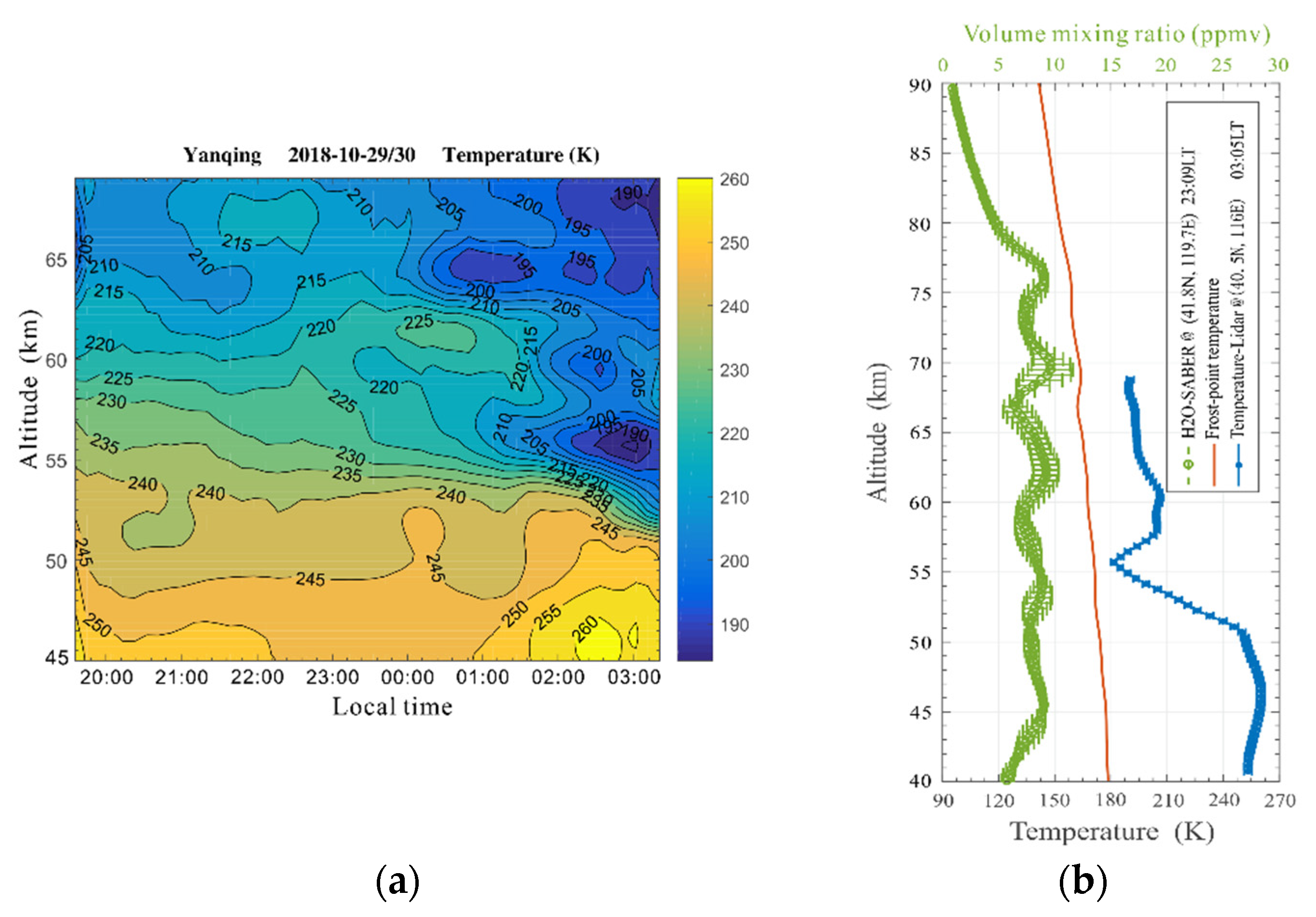
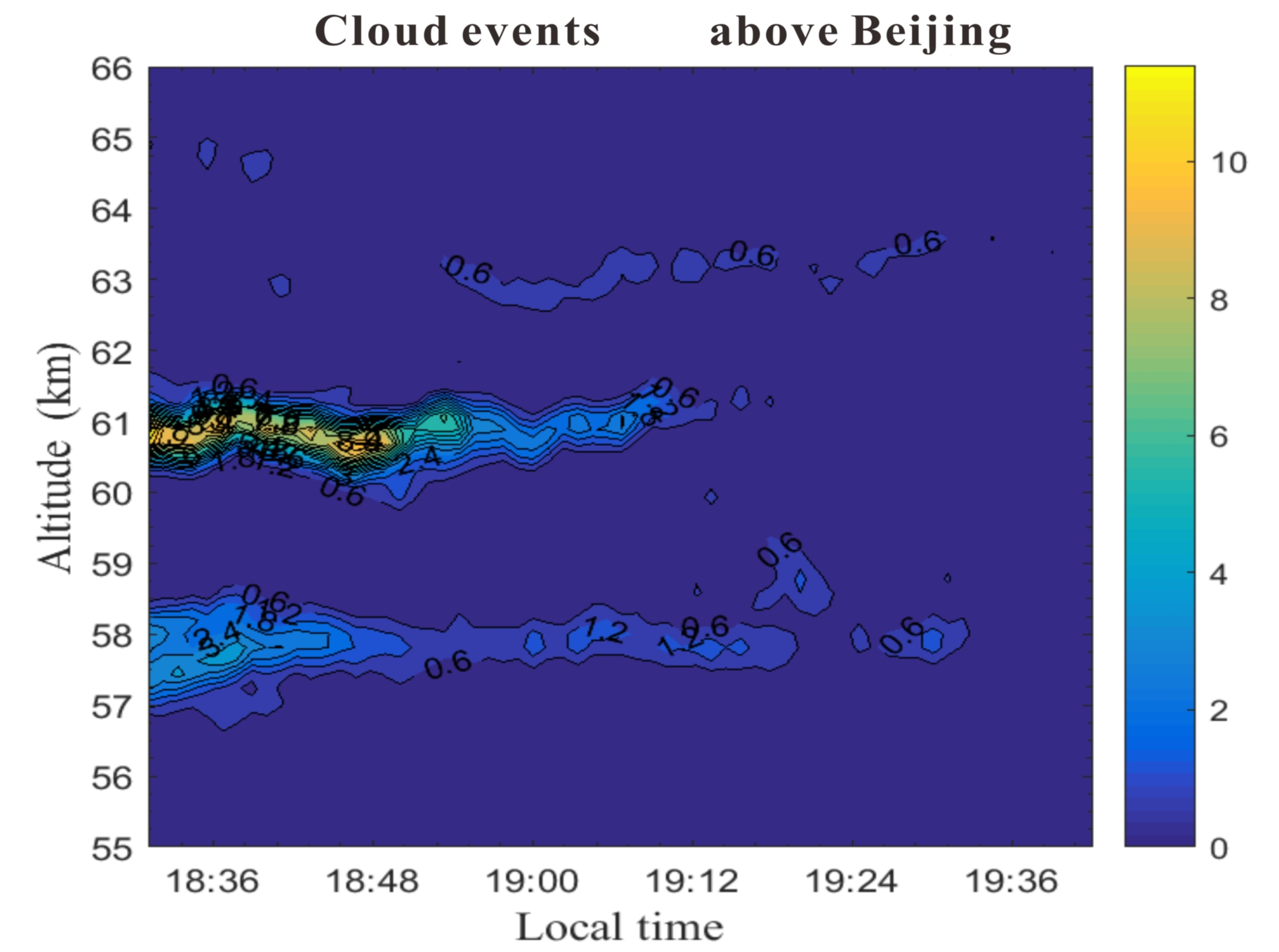
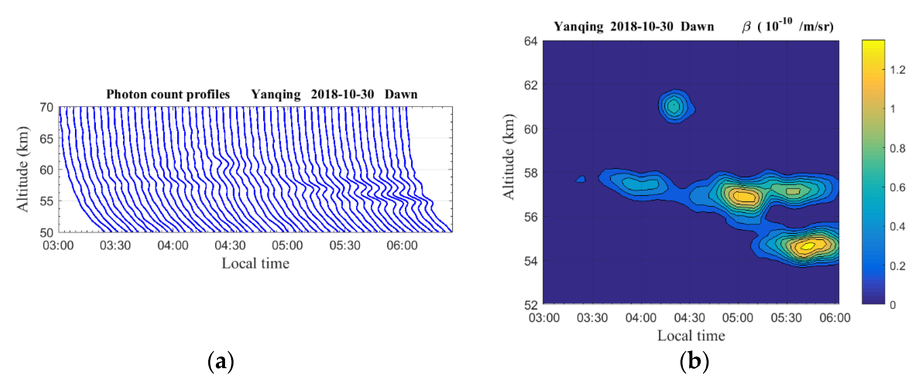
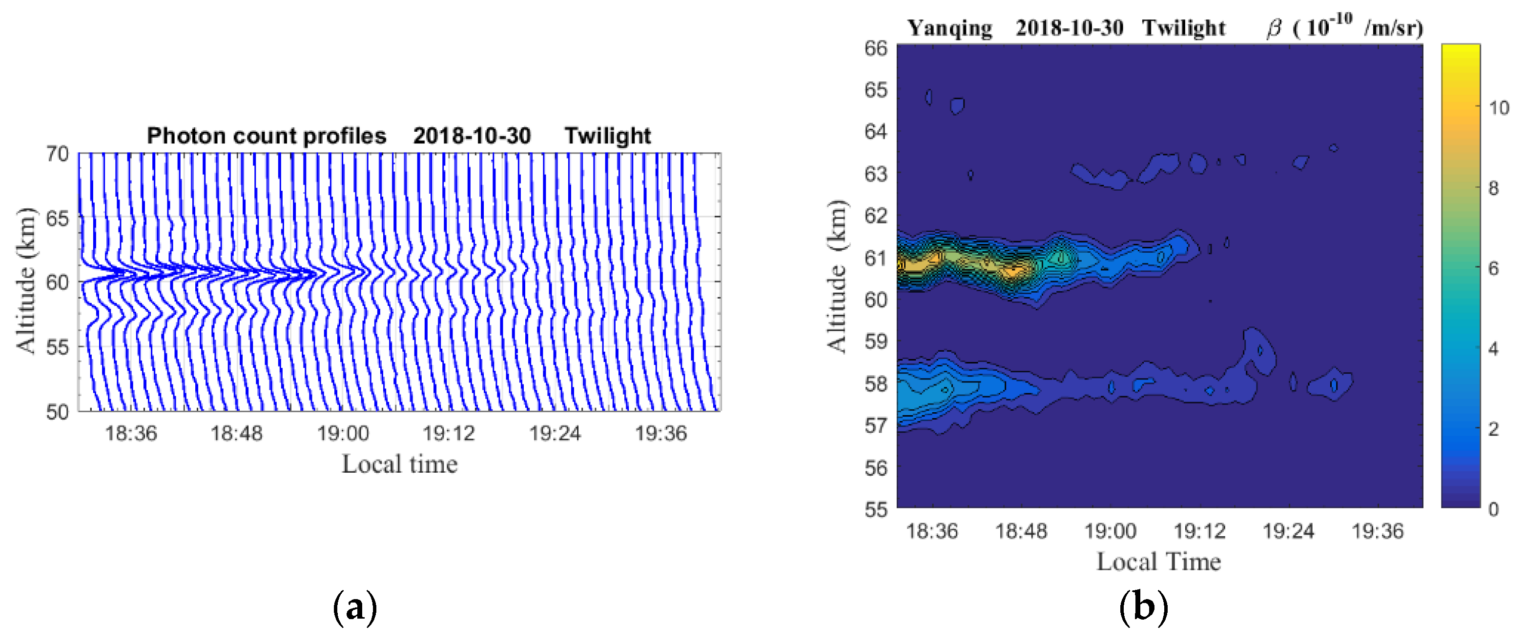
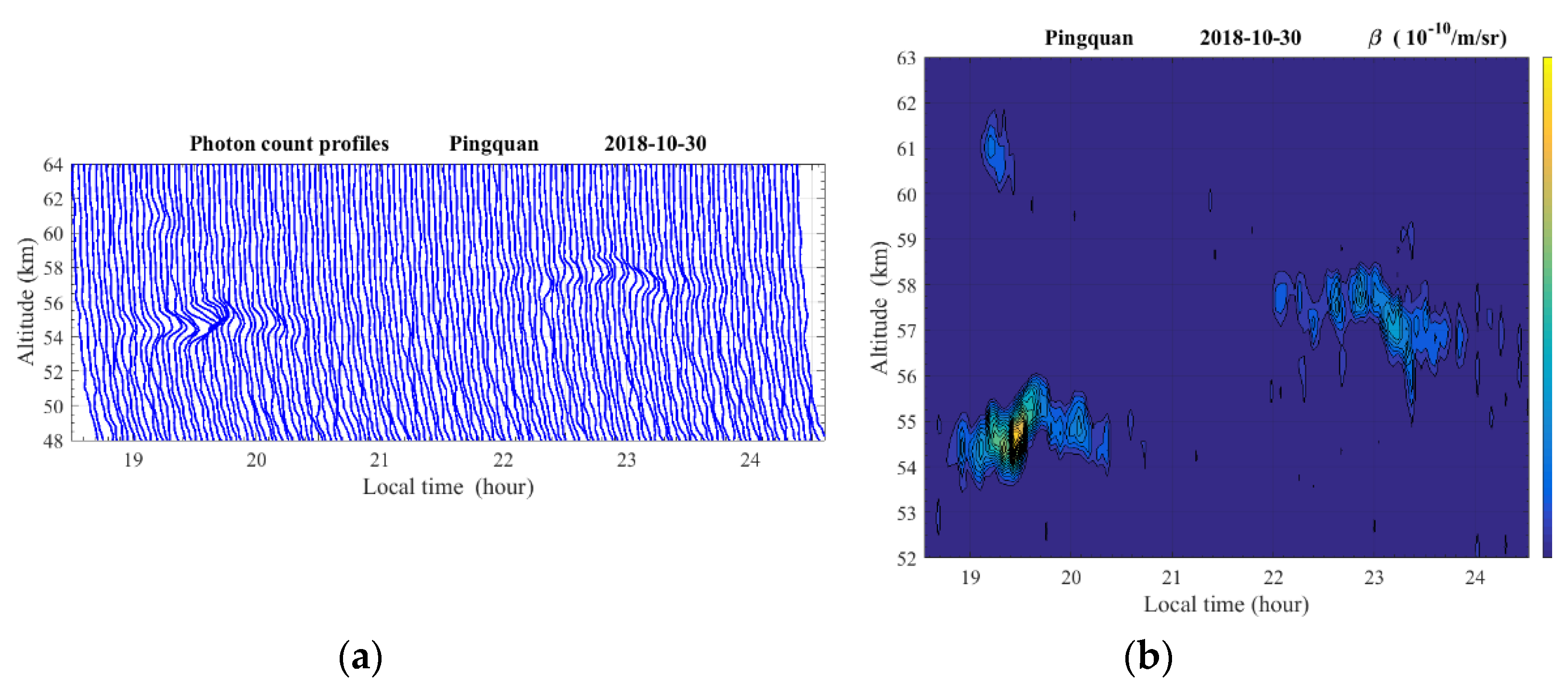
3.1. Cloud Events Observed on 30 October 2018

In Table 1, cloud events were observed by lidars on 3 nights at both Yanqing (40.5°N, 116°E) and Pingquan (41°N, 118.7°E), namely, 27 September 2017, 30 October 2018, and 24 November 2018. Comparing the simultaneous observation results between these two locations, it could be concluded that the cloud events occurred within a similar altitude range, while the fine structure or VBSC of the cloud layers slightly differed. The horizontal distance between Yanqing (40.5°N, 116°E) and Pingquan (41°N, 118.7°E) is ~230 km. Regardless of whether the same cloud event had been simultaneously observed at both locations, the simultaneous observation results may suggest that the cloud events occurred within a large region and probably corresponded to synoptic-scale meteorological changes in the middle atmosphere above Beijing. Here, as an example, lidar-observed cloud events on 30 October 2018 are introduced in detail.

During the regular lidar observation period at Yanqing station (40.5°N, 116°E) at dawn on 30 October 2018, it was found that some obvious enhancements began to occur in the photon count profiles During the regular lidar observation period at Yanqing station (40.5°N, 116°E) at dawn on 30 October 2018, it was found that some obvious enhancements began to occur in the photon count profiles within the altitude range of 50–65 km due to the occurrence of cloud layers, and these enhancements did not change after deliberate laser frequency detuning. The photon count profile sequence and the temporal evolution of the cloud layer structure are shown in Figure 2. At ~03:40 LT, a tenuous cloud layer first occurred in the lidar line view at approximately 58 km. Approximately 1–2 h later, another two cloud layers gradually emerged at altitudes of ~61 km and ~55 km, and these clouds exhibited an obvious multilayer structure, although the cloud layer at ~61 km was very sparse and visible for ~10 min only. This multilayer structure was maintained until the lidar observation was terminated before sunrise (~06:00 LT). Moreover, the VBSC of the cloud layers at altitudes of approximately 55 km and 57 km mainly exhibited an increasing trend over time, but the maximum value reached only $1.4\times {10}^{-10}{\mathrm{m}}^{-1}{\mathrm{sr}}^{-1}$. Because the VBSC was directly related to the number density of cloud particles, as expressed in Equation (1), these observation results suggest that the cloud layers gradually became thicker over time, but the cloud layers remained very tenuous during dawn hours.

Regular lidar observation experiment restarted at twilight (~18:30 LT) at Yanqing (40.5°N, 116°E), and cloud layers were again observed within a similar altitude range (56–65 km) from the very beginning of this observation period. The photon count profile sequence and temporal evolution of the cloud layers are shown in Figure 3. Compared to the cloud event observed at dawn, these cloud layers mainly occurred at altitudes ranging from 57–65 km at twilight, and the multilayer structure (three layers) became increasingly obvious. In particular, the maximum VBSC of the cloud layers reached$11.2\times {10}^{-10}{\mathrm{m}}^{-1}{\mathrm{sr}}^{-1}$ at approximately 61 km at 18:40 LT, and this value was approximately ten times higher than that observed at dawn, indicating that the clouds had greatly expanded in thickness at twilight. However, Figure 3 shows that the VBSC of the cloud layers gradually decreased thereafter, and the cloud layers had completely diffused at ~19:40 LT, i.e., a gradual vanishing process of cloud events was observed by the lidar at twilight.

At Pingquan station (41°N, 118.7°E), clouds in the vicinity of the stratopause were also observed with lidar at nighttime. The photon count profile sequence and temporal variation in the cloud layer structure are shown in Figure 4. Clouds first occurred within the altitude range of 53–62 km at approximately 18:45 LT with a double-layer structure. The upper cloud layer was located at ~61 km, but it was very sparse and visible by lidar for only ~15 min. The main cloud layer occurred within the altitude range of 53–56 km, and it gradually became thicker over time until the maximum VBSC value of $7.2\times {10}^{-10}{\mathrm{m}}^{-1}{\mathrm{sr}}^{-1}$ was observed at 19:30 LT. Then, it began to gradually diffuse and faded away at ~20:45 LT. However, at ~22:00 LT (i.e., ~1 h later), clouds reoccurred within the altitude range of 56–59 km in a single layer. The thickness of this cloud layer increased over time until the maximum VBSC value of $2.6\times {10}^{-10}{\mathrm{m}}^{-1}{\mathrm{sr}}^{-1}$ was observed at ~23:15 LT. Then, it gradually diffused and completely disappeared at ~00:30 LT (+1 day).

More details on the lidar-observed cloud events above Beijing on 30 October 2018 are listed in Table 1. At both dawn and twilight, clouds with multilayer structures mainly occurred within the altitude range of 53–65 km, and the FWHM of each layer was smaller than 1 km. However, the VBSC value of the clouds varied over time, and the cloud layers were sparse at dawn and thick at twilight.

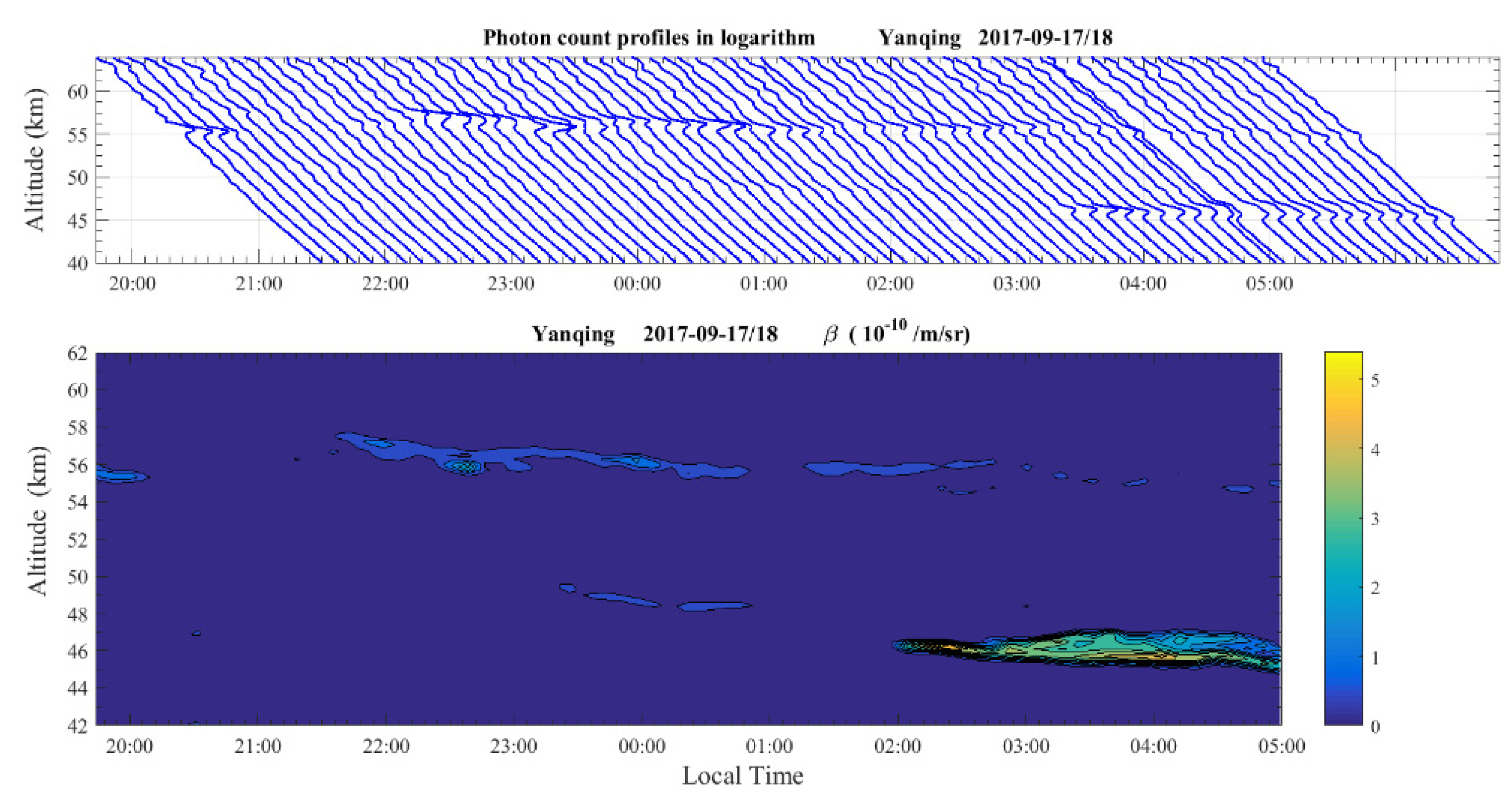
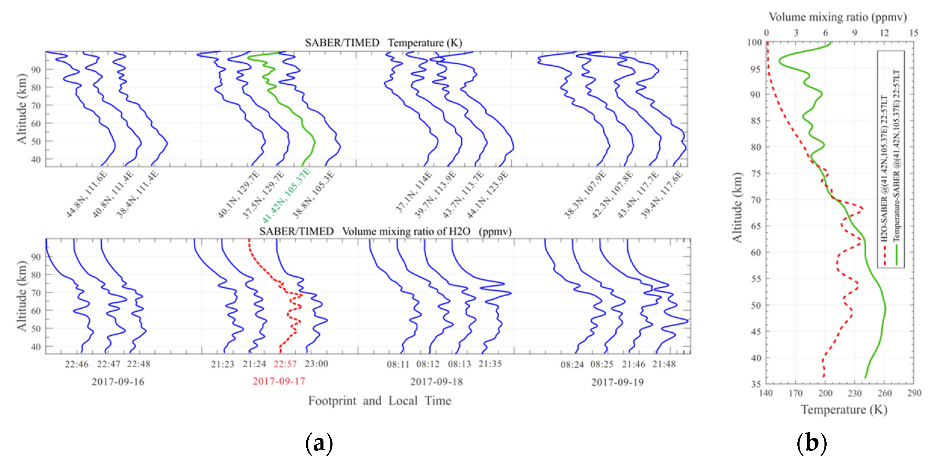
3.2. Cloud Event Observed on 17–18 September 2017

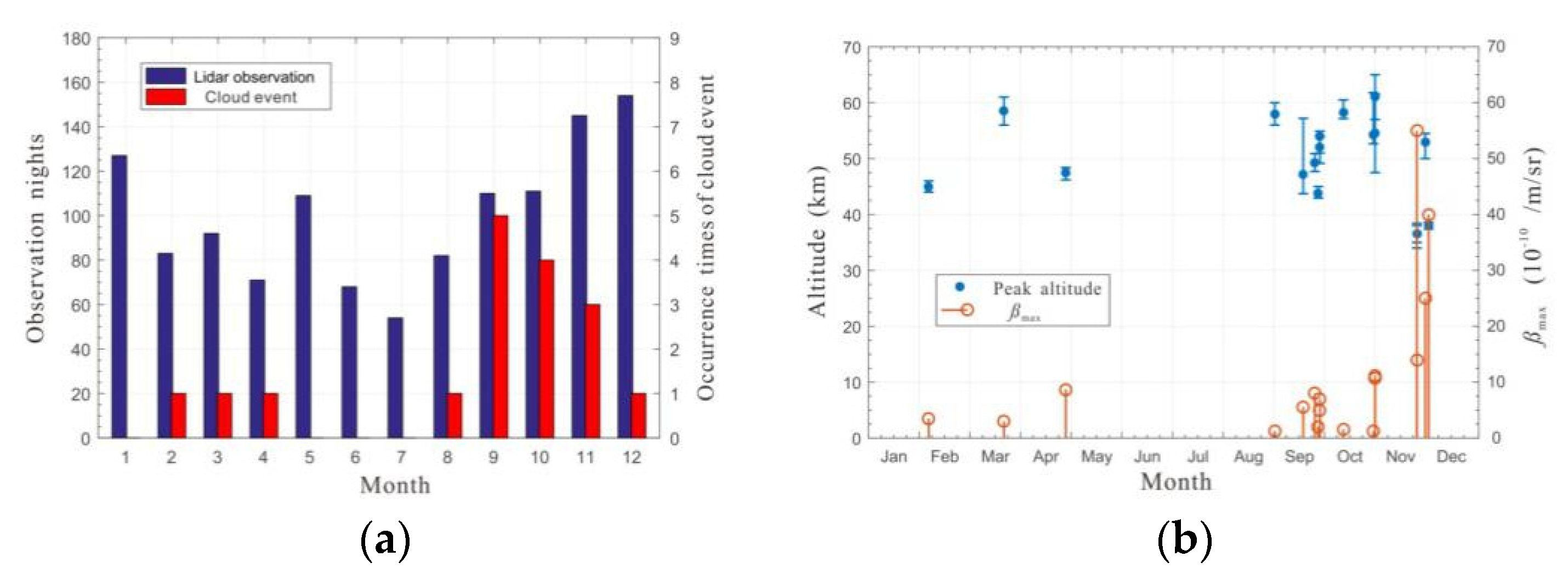
Regarding the duration time, the statistics in Table 1 indicate that these lidar-observed cloud events typically lasted for 1–6 h, but it should be noted that these statistic results were often limited by the lidar observation period because these nighttime lidar observations were typically performed from 19:00 LT to 05:30 LT (+1 day). In regard to the structure of the cloud layers, it was found that cloud layers with double or triple fine structures occurred during 6 cloud events, while the FWHM of each cloud layer was smaller than 1 km, as summarized in Table 1. These results may suggest that these lidar-observed clouds near the stratopause above Beijing were typically faint and tenuous, and at times they were perturbed by wave dynamics. Here, Figure 5 shows a special cloud event that was probably accompanied by wave perturbations throughout the entire nighttime observation period. It was observed at Yanqing (40.5°N, 116°E) during the regular lidar observation period on 17–18 September 2017. In Figure 5, the lidar-measured photon count profile sequence is plotted on a logarithmic scale in the upper panel, and the temporal evolution of the cloud layer structure is correspondingly shown in the bottom panel.

It was found that at approximately 20:00 LT, a very sparse cloud layer first occurred at ~56 km, but it remained visible by lidar for ~15 min only. At ~21:30 LT, this cloud layer reoccurred at altitudes ranging from 54–58 km, and it persisted until the termination of the lidar observation experiment (sunrise). At approximately 23:10 LT, another tenuous and narrow cloud layer emerged within the altitude range of 45–50 km, but it was not visible by lidar during the time period of 1:00–2:00 LT. After its disappearance, this cloud layer became denser and thicker over time until the termination of lidar observation. That is, a cloud event with a double-layer structure was observed with the lidar at night on 17–18 September 2017, and the cloud layers were sparse with a maximum VBSC value of $5.6\times {10}^{-10}{\mathrm{m}}^{-1}{\mathrm{sr}}^{-1}$. In particular, the altitude distribution and fine structure of cloud layers remained relatively steady throughout the entire nighttime observation period.

4. Discussion

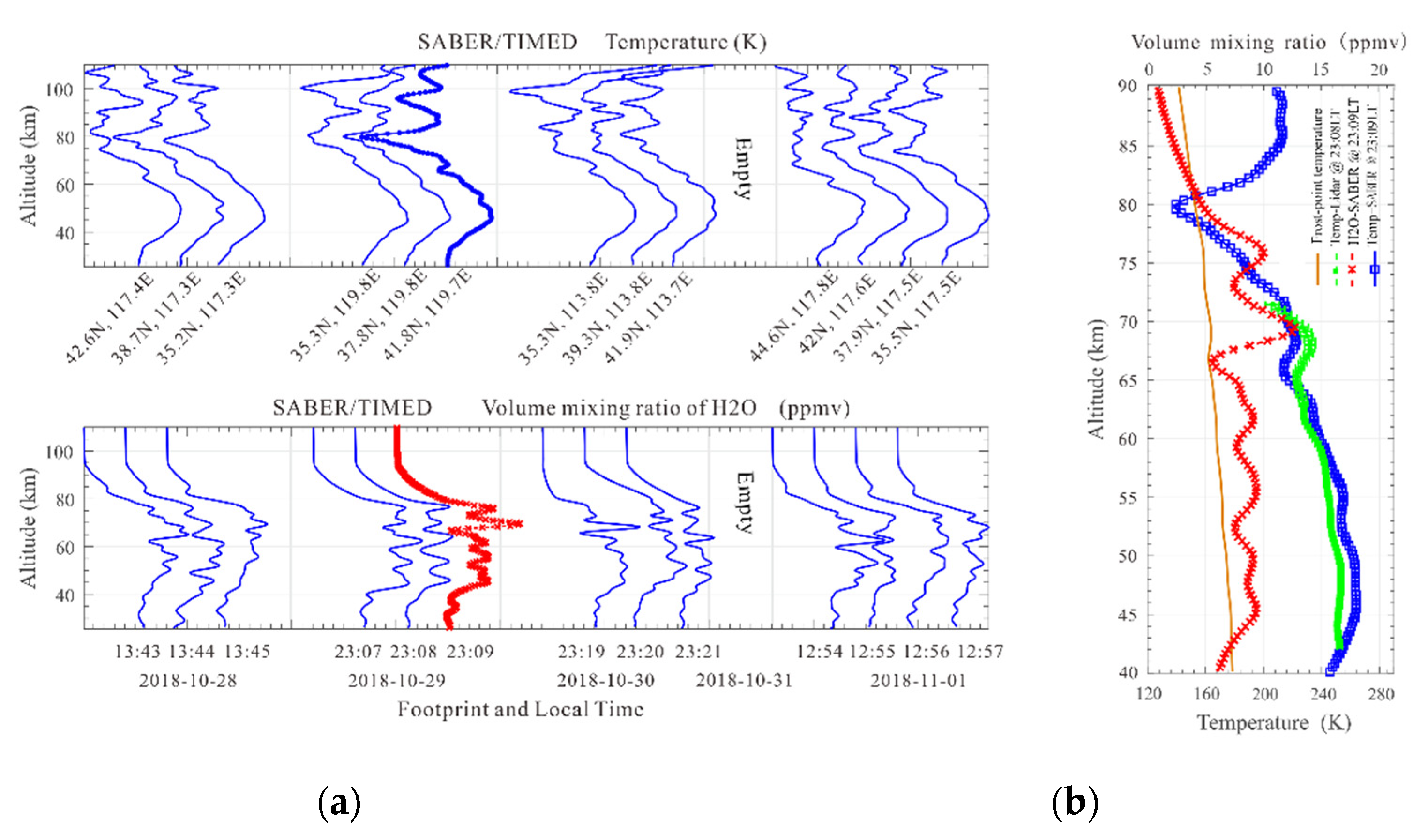
4.1. Occurrence of Cloud Events on 30 October 2018

Currently, the origin of NLCs (or PMCs) is already clear to researchers, i.e., due to an extremely low ambient temperature, supersaturated water vapor condenses and forms ice particles on preexisting nuclei (e.g., cosmic dust or large ions), while the temperature approaches the frost-point temperature ($T_{frost}$). The lidar-observed clouds in the vicinity of the stratopause above Beijing probably exhibit similar formation mechanisms, although the above comparison indicates that they differ from NLCs and PSCs in regard to many features. As a result, the temperature structure (30–68 km) was retrieved according to lidar observations before the onset of cloud events, with the method introduced by Chanin and Hauchecorne [36]. The frost-point temperature at different altitudes can be estimated with Equations (3) and (4) based on the obtained temperature and water vapor measurements from SABER/TIMED [2].

$$D=\frac{p_{H_{2}O}}{p_{sat}}=X·\frac{p_{atm}}{p_{sat}}$$

(3)

$$lo{g}_{10}{p}_{sat}=12.537-\left(2663.5/T\right)$$

(4)

where $D$ is the degree of saturation, $X$ is the volume mixing ratio of water vapor, $p_{sat}$ is the saturation pressure of water vapor over ice, and $p_{atm}$ and $T$ are the atmospheric pressure and temperature, respectively. The frost-point temperature, $T_{frost}$, is the atmospheric temperature at which $D=1$.

Regarding the cloud events observed on 30 October 2018, the atmospheric temperature structure before the onset of the cloud events was first retrieved first with the method described by Chanin and Hauchecorne [36], according to the acquired Rayleigh lidar (@532 nm) observations at Yanqing. The temporal evolution of the temperature structure, as shown in Figure 6a, revealed that within several hours before the occurrence of clouds, the mesosphere exhibited an obvious low-temperature phase within the altitude range of 51–68 km, and the atmospheric temperature in the vicinity of the stratopause (i.e., at altitudes ranging from 52–65 km) quickly decreased over time. In particular, at an altitude of ~58 km, where cloud layers were first observed by lidar, as shown in Figure 2, the atmospheric temperature decreased to ~181 K before cloud event onset. This temperature was extremely low and facilitated the formation of cloud particles near the stratopause. Here, it should be noted that the temperature structure derivation was based on the ideal gas hypothesis, and the temperature structure derivation in Figure 6a was interrupted because of the occurrence of cloud particles at ~03:30 LT [2,36,37].

The SABER/TIMED measurements from 28 October to 1 November were utilized to analyze this lidar-observed cloud event, and the profile sequences of the atmospheric temperature (upper panel) and water vapor (bottom panel) are shown in Figure 7a. Here, the SABER measurements were limited to the region of 35–45°N in latitude and 112–122°E in longitude, and the footprints and local time stamps are correspondingly marked on the horizontal axis. Comparing the measurement results among the different dates, it could be found that an obvious temperature anomaly with an extremely low temperature of ~139 K occurred at approximately 80 km on 29 October 2018, and the atmospheric temperature quickly decreased from 220 K to 139 K within the altitude range of 70–80 km, corresponding to a cooling rate of ~8 K/km along the vertical direction. Moreover, the volume mixing ratio of water vapor typically ranged from 7–10 ppmv within the altitude range of 45–75 km, with a maximum value of 12.3 ppmv occurring at 69 km. Since this SABER measurement was obtained at the footprint (41.8°N, 119.7°E) at 23:09 LT (i.e., ~4 h before the onset of the cloud event) close to cloud event onset in both location and time, atmospheric temperature (blue solid line with circles) and water vapor (red dashed line with crosses) profiles were plotted for comparison, as shown in Figure 7b. At altitudes ranging from 65–78 km, abundant water vapor corresponded to a temperature cooling rate of ~8 K/km, indicating that water vapor became saturated due to intense vertical convection of air masses several hours before the cloud event [38].

Combining the above lidar and SABER measurement results, it may be concluded that the meteorological changes in the middle atmosphere facilitated the onset of cloud events on 30 October 2018. To focus on the frost-point temperature of water vapor, it was calculated with Equations (3) and (4) according to the SABER measurements and plotted in Figure 6b with a red line. The estimation results illustrated that the frost-point temperature gradually increased with decreasing altitude, and values of ~150 K and ~173 K were at altitudes of 80 km and 55 km, respectively. For comparison, the SABER-measured water vapor profile (@(41.8°N, 119.7°E) & 23:09 LT) and lidar-measured temperature profile (@(40.5°N, 116°E) & 03:05 LT) were also shown in Figure 6b. The lidar-measured atmospheric temperature (~181 K) was close to the estimated frost-point temperature (~173 K) at an altitude of ~56 km, while the average volume mixing ratio of water vapor reached ~8.5 ppmv in the vicinity of the stratopause. Considering the probable uncertainties in both the lidar and SABER measurements, as well as the calculation deviation in the empirical equation Equation (4), it could be inferred that the atmospheric temperature near the stratopause probably decreased to a critical value ($T_{frost}$) after 03:40 LT. Therefore, the onset mechanism of the cloud event on 30 October 2018 may be deduced as follows: abundant saturated water vapor condensed into cloud particles in the vicinity of the stratopause above Beijing while the mesosphere was subjected to a low-temperature phase.

In contrast, Figure 2 and Figure 3 show that this cloud event occurred within a similar altitude range both at dawn and twilight on 30 October 2018, and its beginning and vanishing processes were clearly recorded by lidar observation at Yanqing (40.5°N, 116°E). Considering that cloud events at similar altitudes were simultaneously observed at two lidar stations that are separated horizontally by a distance of ~230 km, it could be deduced that the occurrence of cloud events on 30 October 2018 was perhaps associated with a long in duration and large scale, corresponding to synoptic-scale meteorological changes in the middle atmosphere above Beijing.

In addition, as shown in Figure 6 and Figure 7, the horizontal bars marked in the lidar-measured temperature profiles indicate the uncertainty in the temperature at the different altitudes, and the uncertainty in the retrieved temperature profile was typically less than 6 K at altitudes ranging from 40–70 km [17,37]. In contrast, lidar-measured temperature profiles at 23:09 LT are compared to simultaneous SABER observation results in Figure 7b, and similar temperature variations were found within the altitude range of 45–70 km. The temperature difference between the two simultaneous measurements was mainly related to the fact that the temperature profiles measured by the lidar at Yanqing (40.5°N, 116°E) were obtained using the vertical detection method, and the SABER measurement results were obtained via the limb-scanning measurement technique when the TIMED satellite passed over the footprint (41.8°N, 119.7°E).

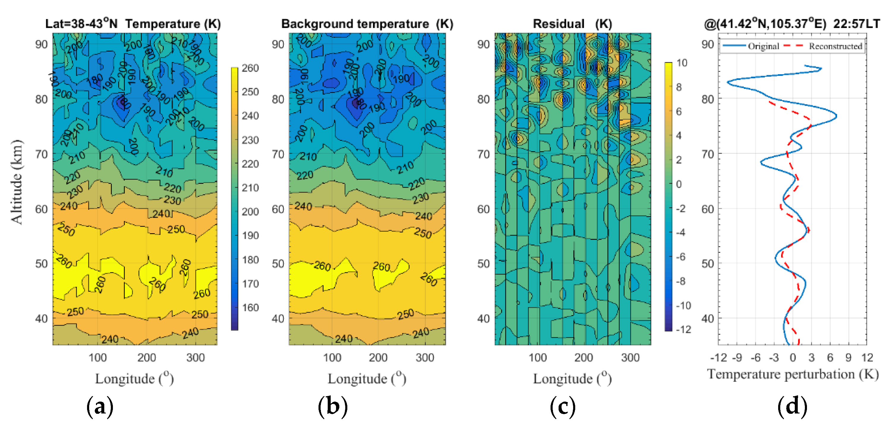
4.2. Occurrence of Cloud Event on 17–18 September 2017

Regarding the cloud event observed on 17/18 September 2017, SABER measurements of the temperature and water vapor over Beijing from October 28 to November 1 are shown in Figure 8a. Similarly, the footprints of these measurements were also limited to 35–45°N in latitude and 112–122°E in longitude. Since the measurement at the footprint (41.42°N, 105.37°E) is the closest to the lidar-observed cloud event in both location and time, temperature and water vapor profiles measured at 22:57 LT on 17 September 2017 are plotted in detail in Figure 8b. The volume mixing ratio of water vapor ranged from 7–10 ppmv at altitudes from 50–70 km, suggesting that water vapor was sufficient in the lower mesosphere above Beijing. However, no obvious temperature anomaly was found in the middle atmosphere except for a lower temperature of ~150 K, which occurred at approximately 96 km. Therefore, these conditions did not satisfy the strict requirements for water vapor nucleation in the vicinity of the stratopause, and the onset of this cloud event was unrelated to the influences of the temperature anomaly in the middle atmosphere.

Nevertheless, Figure 5 shows that the clouds maintained a wave-like structure (double layers) within the altitude range of 40–60 km throughout almost the entire lidar observation period (~8 h), indicating that this cloud event was probably perturbed by persistent gravity wave propagations in the middle atmosphere. It is widely accepted that wave perturbation is a ubiquitous dynamical feature of the middle atmosphere, and complex interactions among gravity waves, tides, and planetary waves are crucial drivers of atmospheric thermal structure variations [39]. The simulations conducted by Hoffmann et al. [40] revealed that tides and gravity waves played a key role in the formation of polar mesospheric summer echo (PMSE) layers and NLCs, and the presence of gravity waves could enhance the formation of multiple PMSE layer structures. It has also been proven by many observations that the NLC (or PMC) and PSC layers indeed follow the motion of the cold phase of wave perturbations [12,41,42]. As a result, to investigate gravity wave activities during the nighttime, temperature data measured by SABER on 17/18 September 2017 were analyzed with the harmonic analysis method [17,43].

First, the temperature structure (35–90 km) measured at descending nodes near 40.5°N is shown in Figure 9a, and the background temperature Figure 9b was obtained after the least square harmonic fitting was applied to the temperature structure at each altitude. Then, by removing the background temperature from the observed temperature, the residuals Figure 9c could be regarded as the temperature perturbations induced by gravity waves. To closely consider the SABER measurement results over Beijing, the temperature perturbation profile measured at the footprint (41.42°N, 105.37°E) at 22:57 LT was plotted with a blue curve in Figure 9d. After wavelet analysis (i.e., Morlet) of the temperature perturbation profile, the main wave components could be obtained, and a new temperature perturbation profile was finally reconstructed, as shown in Figure 9d, with the three dominant wave components [44].

Analysis results in Figure 9 shows that at 22:57 LT, the middle atmosphere (35–80 km) above Beijing was indeed perturbed by gravity waves with vertical wavelengths of ${\lambda }_z=7-10 \mathrm{km}$. During harmonic analysis in this study, it should be noted that the temperature profiles in the latitude band of 38–43°N were selected for analysis, and they were rearranged in increasing order of the longitude to produce a longitude-altitude temperature distribution. Moreover, this rearrangement operation was only applied to the data measured at descending nodes, and the mean latitude was 40.3°N with a standard deviation of ~1.5°. During least square harmonic fitting, the zonal wavenumbers were set to k = 0, 1, 2, 3, 4, 5, 6, and 7, such that tides and planetary waves could be efficiently eliminated since they generally exhibit longer horizontal wavelengths.

To compare the simultaneous lidar observations with the above harmonic analysis results, as shown in Figure 5, a similar wave-like structure of cloud layers occurred within the same altitude range (40–65 km), confirming that these cloud layers were perturbed by gravity wave propagations above Beijing at night on 17 September 2017. Namely, two cloud layers respectively occurred at altitudes of ~48 km and ~57 km at approximately 23:00 LT in Figure 5, corresponding to a peak altitude difference of ~8.5 km. However, at altitudes ranging from 40–65 km, the antinodes of the wave perturbations (red dashed line) were respectively located at ~52 km and ~61 km in Figure 9d, indicating that the lidar-observed peak altitudes of the cloud layers did not suitably match the lower temperature points induced by the wave perturbations. That is, in contrast to the observation results of NLCs and PSCs, the lidar-observed cloud layer above Beijing did not follow the motion of the cold phase of wave perturbations. Moreover, in Figure 9d, amplitudes of temperature perturbation were only 3–5 K at altitudes of 40–65 km. Compared to the background temperature (~220–260 K) in Figure 9b, the cooling effect of gravity wave activities was too weak for water vapor to nucleate into ice particles. Therefore, for these lidar-observed clouds at night on 17–18 September 2017, they possibly did not comprise ice particles condensed from water vapor, and the occurrence of this cloud event could not be ascribed to the dynamic process in the middle atmosphere, although the cloud layers were indeed perturbed by gravity waves and persistently exhibited a double-layer fine structure.

In practice, except for ice particles, mesospheric cloud clusters composed of other tiny particles also can be identified from lidar’s backscatter signals. As we know, there is a large number of minuscule particles floating in the middle atmosphere, such as aerosol particles, cosmic dust, hydrate droplets, volcanic ash, and they have similar scattering properties to ice particles during lidar observations. According to the temporal evolution of cloud layer structures depicted in Figure 5, it is inferred that a cluster of minuscule particles was observed by the lidar in the middle atmosphere, which gradually drifted toward the observation site. Moreover, the altitude distribution and fine structure of the cloud layers remained relatively steady throughout the entire nighttime observation period (~8 h), suggesting that this cluster of minuscule particles could be very large in scale considering the effects of horizontal winds. Therefore, the onset of this cloud event was not related to the condensing of water vapor, and these lidar-observed clouds in the vicinity of the stratopause above Beijing could be floating clusters of aerosol particles, cosmic dust, hydrate droplets, volcanic ash, etc.

4.3. Occurrence Mechanism

Indeed, over the past few decades, the mesopause has increasingly cooled due to increasing levels of CO₂, and more water vapor has occurred in the mesosphere due to the oxidation of elevated levels of methane. Similar to recent changes in NLCs (or PMCs), an increasing number of these cloud events may be observed at midlatitudes in the future because of these systematic climate changes. Regarding the cloud events on 30 October 2018, cloud layers should be generated locally via water vapor condensation. First, abundant water vapor (6–12.3 ppmv) and an extremely low temperature anomaly (~139 K) were detected by SABER near the altitudes where cloud layers occurred. Second, lidar measurements indicated that the middle atmosphere experienced a cooling process, and the atmospheric temperature (181 K) approached the frost point at the altitude where the cloud layer first occurred. Third, both the onset and the vanishing processes of this cloud event were clearly observed by lidar at Yanqing. Notably, cloud events were simultaneously observed within similar altitude ranges at the two lidar stations that are separated horizontally by ~230 km. These analysis results were used to deduce that the onset of this cloud event could be attributed to local meteorological changes in the middle atmosphere above Beijing, and the cloud layers resulted from local water vapor condensation.

However, regarding the cloud layers observed on 17–18 September 2017, the analysis results revealed that they likely did not result from the local nucleation of water vapor at extremely low ambient temperatures, although water vapor was also sufficient in the middle atmosphere. First, there was not any obvious cooling process that occurred in the vicinity of the stratopause before the onset of the cloud event. Second, cloud layers were perturbed by gravity waves, while the cloud layer did not follow the motion of the cold phase of wave perturbations. Third, the altitude distribution and fine structure of cloud layers remained relatively steady throughout the entire nighttime observation period. Therefore, instead of ice particles, these lidar-observed cloud clusters probably mainly comprised minuscule particles of aerosol particles, cosmic dust, hydrate droplets, volcanic ash, etc.

Since the onset of the two typical cloud events is attributed to different mechanisms above, features in their cloud layers’ temporal evolutions are compared. In Figure 2, Figure 3 and Figure 4, the structure and VBSC of cloud layers changed obviously with time, and the fine structures above 60 km were typically sparse and visible by lidar for a few minutes only. However, in Figure 4, the VBSC of cloud layers gradually increased with time, and the fine structure remained relatively steady throughout the entire nighttime observation period. For the former, the onset of cloud events likely depended on the local meteorological changes, and the features of cloud layers varied with the transient changes in temperature and water vapor. For the latter, fine structure and altitude distribution of clouds remained relatively steady because their main components were possibly insensitive to the transient changes in temperature and water vapor in the middle atmosphere. Moreover, compared to the other dates in Figure 7, the temperature and water vapor in the middle atmosphere varied obviously on 30 October 2018. However, in Figure 8, there was not obvious change found in the variations of mesospheric temperature and water vapor on the day of the cloud event. In the same method, SABER measurements of temperature and water vapor were carefully examined for every cloud event in Table 1, and it is found that, except for the cloud event on 30 October 2018, the onset of 3 cloud events (i.e., 11 October 2013, 27 September 2017, 24 November 2018) was probably related to the local meteorological changes in the middle atmosphere.

Of course, it could be possible that some lidar-observed clouds resulted from space traffic exhaust. Many observations have proven that rocket exhaust (e.g., detachment of a solid rock booster) can occasionally generate minuscule individual clouds in the middle atmosphere, and the interannual variability in PMCs can be affected by space traffic [19,20,45,46]. In Table 1, for those cloud events observed by lidar on 26 September 2010, 22 March 2014 and 05 February 2018, tenuous clouds with a single layer and short duration could be generated by rocket exhaust emissions in the vicinity of the stratosphere. However, for those events marked with a star in Table 1 (i.e., 27 September 2017, 30 October 2018 and 24 November 2018), cloud events were simultaneously observed by lidar at both Yanqing (40.5°N, 116°E) and Pingquan (41°N, 118.7°E), and they should be large in scale and likely not related to rocket exhaust.

In fact, these lidar-observed cloud events in the vicinity of the stratopause above Beijing may be associated with additional possible formation mechanisms, except for those described above, and the microphysical processes behind these rare phenomena are probably complicated as well. Further investigations on the composition and specific formation mechanism are needed in the future due to the limits of detection instruments and the lack of accurate information on local temperature, water vapor and wind fields.

5. Summary and Conclusions

Based on the lidar observations at Yanqing (40.5°N, 116°E) and Pingquan (41°N, 118.7°E) from 2009–2018, cloud events in the vicinity of the stratopause above Beijing were first reported. In total, 17 cloud events were identified from 1488 nighttime observations. The statistical results indicated that they mainly occurred within the altitude range of 33–65 km in autumn and early winter and were seldom observed by lidar during the months of May to July. The cloud layers were typically tenuous and sparse, and their maximum VBSC values ranged from $1\times {10}^{-10}{\mathrm{m}}^{-1}{\mathrm{sr}}^{-1}$ to $5.5\times {10}^{-9}{\mathrm{m}}^{-1}{\mathrm{sr}}^{-1}$. These cloud events are rare mesospheric phenomena observed by lidars at relatively low latitudes, and they differ from NLCs and PSCs in terms of the altitude distribution and seasonal variation.

The occurrence mechanism of these lidar-observed cloud events was examined by analyzing temperature and water vapor measurements retrieved from SABER/TIMED. Regarding the cloud event observed on 30 October 2018, it was attributed to meteorological changes above Beijing, and the cloud layers resulted from the condensation of water vapor in the vicinity of the stratopause. Regarding the cloud event observed on 17–18 September 2017, these lidar-observed clouds were deduced to be a cluster of minuscule particles disturbed by gravity waves, and the onset of this cloud event was possibly not related to the nucleation of local water vapor. Therefore, for these lidar-observed cloud events, some cloud layers resulted from the nucleation of water vapor due to the local meteorological changes in the middle atmosphere, while other lidar-observed cloud layers could comprise floating clusters of cosmic dust, hydrate droplets, volcanic ash, space traffic exhaust, etc.

Over the past few decades, the global climate has systematically changed due to rising greenhouse gas concentrations in the atmosphere, and the relevant microphysics processes behind the occurrence of these cloud events were probably significant to the climate changes at midlatitudes in China. In the future, more observations and studies of similar cloud events in Beijing should be performed, including the determination of the components and particle size of clouds, annual and seasonal variation features, and possible formation mechanisms. In practice, local temperature and water vapor measurements are important to the study of these unusual atmospheric phenomena because the onset of cloud events is likely related to the instantaneous changes in synoptic-scale temperature and water vapor within a certain small region. However, in many cases, the values measured by satellites at their footprints differ from the real temperature and water vapor values where clouds locally form because of the large spatial gaps between adjacent orbits at midlatitudes. Lidar measurements of the temperature structure in the mesosphere are also limited due to the occurrence of cloud particles. Therefore, in further investigations, numerous models and simultaneous measurements involving cameras and falling spheres (or sounding rockets) will be helpful.

References

1. Straka, J.M. Cloud and Precipitation Microphysics: Principles and Parameterizations; Cambridge University Press: Cambridge, UK, 2009. [Google Scholar]
2. Lübken, F.J.; Fricke, K.H.; Langer, M. Noctilucent clouds and the thermal structure near the Arctic mesopause in summer. J. Geophys. Res. 1996, 101, 9489–9508. [Google Scholar] [CrossRef]
3. Cossart, G.; Fiedler, J.; Zahn, U. Size distributions of NLC particles as determined from 3-color observations of NLC by ground-based lidar. Geophys. Res. Lett. 1999, 26, 1513–1516. [Google Scholar] [CrossRef]
4. Demissie, T.D.; Espy, P.J.; Kleinknecht, N.H.; Kaifler, M.; Kaifler, N.; Baumgarten, G. Characteristics and sources of gravity waves observed in NLC over Norway. Atmos. Chem. Phys. 2014, 14, 12133–12142. [Google Scholar] [CrossRef] [Green Version]
5. Lübken, F.J.; Höffner, J.; Viehl, T.P.; Kaifler, B.; Morris, R.J. Winter/summer mesopause temperature transition at Davis (69° S) in 2011/2012. Geophys. Res. Lett. 2015, 41, 5233–5238. [Google Scholar] [CrossRef] [Green Version]
6. Backhouse, T.W. The luminous cirrus cloud of June and July. Meteorol. Mag. 1885, 20, 133. [Google Scholar]
7. Thomas, L.; Marsh, A.K.P.; Wareing, D.P.; Hassan, M.A. Lidar observations of ice crystals associated with noctilucent clouds at middle latitudes. Geophys. Res. Lett. 1994, 21, 385–388. [Google Scholar] [CrossRef]
8. Thayer, J.P.; Nielsen, N.; Jacobsen, J. Noctilucent cloud observations over Greenland by a Rayleigh lidar. Geophys. Res. Lett. 1995, 22, 2916–2964. [Google Scholar] [CrossRef]
9. Gerding, M.; Höffner, J.; Hoffmann, P.; Kopp, M.; Lübken, F.J. Noctilucent cloud variability and mean parameters from 15 years of lidar observations at a mid-latitude site (54° N, 12° E). J. Geophys. Res. 2013, 118, 317–328. [Google Scholar] [CrossRef]
10. Gadsden, M. The North-West Europe data on noctilucent clouds: A survey. J. Atmos. Sol. Terr. Phys. 1998, 60, 1163–1174. [Google Scholar] [CrossRef]
11. McCormick, M.P.; Steele, H.M.; Hamill, P.; Chu, W.P.; Swissler, T.J. Polar stratospheric cloud sightings by SAM II. J. Atmos. Sci. 1982, 39, 1387–1397. [Google Scholar] [CrossRef]
12. Collins, R.L.; Bowman, K.P.; Gardner, C.S. Polar stratospheric clouds at the South Pole in 1990. J. Geophys. Res. 1993, 98, 1001–1010. [Google Scholar] [CrossRef]
13. Hoffmann, L.; Spang, R.; Orr, A.; Alexander, M.J.; Holt, L.A.; Stein, O. A decadal satellite record of gravity wave activity in the lower stratosphere to study polar stratospheric cloud formation. Atmos. Chem. Phys. 2017, 17, 2901–2920. [Google Scholar] [CrossRef] [Green Version]
14. Lowe, D.; MacKenzie, A.R. Review of polar stratospheric cloud microphysics and chemistry. J. Atmos. Sol. Terr. Phys. 2008, 70, 13–40. [Google Scholar] [CrossRef] [Green Version]
15. Pitts, M.C.; Poole, L.R.; Thomason, L.W. CALIPSO polar stratospheric cloud observations: Second-generation detection algorithm and composition discrimination. Atmos. Chem. Phys. 2009, 9, 7577–7589. [Google Scholar] [CrossRef] [Green Version]
16. Yue, C.; Yang, G.; Wang, J.; Guan, S.; Du, L.; Cheng, X.; Yang, Y. Lidar observations of the middle atmospheric thermal structure over north China and comparisons with TIMED/SABER. J. Atmos. Sol. Terr. Phys. 2014, 120, 80–87. [Google Scholar] [CrossRef]
17. Gong, S.; Yang, G.; Xu, J.; Liu, X.; Li, Q. Gravity wave propagation from the stratosphere into the mesosphere studied with lidar, meteor radar, and TIMED/SABER. Atmosphere 2019, 10, 81. [Google Scholar] [CrossRef] [Green Version]
18. Thomas, G.E. Mesospheric clouds and the physics of the mesopause region. Rev. Geophys. 1991, 29, 553–575. [Google Scholar] [CrossRef]
19. Siskind, D.E.; Stevens, M.H.; Emmert, J.T.; Drob, D.P.; Kochenash, A.J.; Russell, J.M., III; Gordley, L.L.; Mlynczak, M.G. Signatures of shuttle and rocket exhaust plumes in TIMED/SABER radiance data. Geophys. Res. Lett. 2003, 30, 1819. [Google Scholar] [CrossRef]
20. Siskind, D.E.; Stevens, M.H.; Hervig, M.E.; Randall, C.E. Recent observations of high mass density polar mesospheric clouds: A link to space traffic? Geophys. Res. Lett. 2013, 40, 2813–2817. [Google Scholar] [CrossRef]
21. Burke, E.J.; Chadburn, S.E.; Huntingford, C.; Jones, C.D. CO2 loss by permafrost thawing implies additional emissions reductions to limit warming to 1.5 or 2 °C. Environ. Res. Lett. 2018, 13, 024024. [Google Scholar] [CrossRef]
22. Forster, P.M.; Maycock, A.C.; McKenna, C.M.; Smith, C.J. Latest climate models confirm need for urgent mitigation. Nat. Clim. Change 2020, 10, 7–10. [Google Scholar] [CrossRef]
23. Butler, J.H.; Montzka, S.A. The NOAA Annual Greenhouse Gas Index (AGGI); National Oceanic and Atmospheric Administration, Earth System Research Laboratories: Boulder, CO, USA, 2020. [Google Scholar]
24. She, C.Y.; Berger, U.; Yan, Z.A.; Yuan, T.; Lübken, F.J.; Krueger, D.A.; Hu, X. Solar response and long-term trend of midlatitude mesopause region temperature based on 28 years (1990–2017) of Na lidar observations. J. Geophys. Res. Space Phys. 2019, 124, 7140–7156. [Google Scholar] [CrossRef]
25. Yuan, T.; Solomon, S.C.; She, C.Y.; Krueger, D.A.; Liu, H.L. The long-term trends of nocturnal mesopause temperature and altitude revealed by Na lidar observations between 1990 and 2018 at midlatitude. J. Geophys. Res. Atmos. 2019, 124, 5970–5980. [Google Scholar] [CrossRef] [Green Version]
26. Wickwar, V.B.; Taylor, M.J.; Herron, J.P.; Martineau, B.A. Visual and lidar observations of noctilucent clouds above Logan, Utah, at 41.7° N. J. Geophys. Res. 2002, 107, 4054. [Google Scholar] [CrossRef]
27. Taylor, M.J.; Gadsden, M.; Lowe, R.P.; Zalcik, M.S.; Brausch, J. Mesospheric cloud observations at unusually low latitudes. J. Atmos. Sol. Terr. Phys. 2002, 64, 991–999. [Google Scholar] [CrossRef]
28. Russell, M.J., III; Rong, P.; Hervig, M.E.; Siskind, D.E.; Stevens, M.H.; Bailey, S.M.; Gumbel, J. Analysis of northern mid-latitude noctilucent cloud occurrences using satellite data and modeling. J. Geophys. Res. 2014, 119, 3238–3250. [Google Scholar] [CrossRef]
29. Suzuki, H.; Sakanoi, K.; Nishitani, N.; Ogawa, T.; Ejiri, M.K.; Kubota, M.; Kinoshita, T.; Murayama, Y.; Fujiyoshi, Y. First imaging and identification of a noctilucent cloud from multiple sites in Hokkaido (43.2–44.4° N), Japan. Earth Planets Space 2016, 68, 182. [Google Scholar] [CrossRef] [Green Version]
30. Cossart, G.; Fiedler, J.; von Zahn, U.; Keckhut, P.; Haucheorne, A. Mid-latitude noctilucent cloud observations by lidar. Geophys. Res. Lett. 1996, 23, 2919–2922. [Google Scholar] [CrossRef]
31. Chu, X.; Gardner, C.S.; Papen, G. Lidar observations of polar mesospheric clouds at South Pole: Diurnal variations. Geophys. Res. Lett. 2001, 28, 1937–1940. [Google Scholar] [CrossRef] [Green Version]
32. Gong, S.; Yang, G.; Xu, J.; Wang, J.; Guan, S.; Gong, W.; Fu, J. Statistical characteristics of atmospheric gravity wave in the mesopause region observed with a sodium lidar at Beijing, China. J. Atmos. Sol. Terr. Phys. 2013, 97, 143–151. [Google Scholar] [CrossRef]
33. Russell, J.M.; Mlynczak, M.G.; Gordley, L.L.; Tansock, J.; Esplin, R. An overview of the SABER experiment and preliminary calibration results. Proc. SPIE 1999, 3756, 277–288. [Google Scholar]
34. Remsberg, E.E.; Marshall, B.T.; Garcia-Comas, M.; Krueger, D.; Lingenfelser, G.S.; Martin-Torres, J.; Mlynczak, M.G.; Russell, J.M.; Smith, A.; Zhao, Y.; et al. Assessment of the quality of the version 1.07 temperature-versus-pressure profiles of the middle atmosphere from TIMED/SABER. J. Geophys. Res. 2008, 113, D17101. [Google Scholar] [CrossRef]
35. Höffner, J.; Fricke-Begemann, C.; Lübken, F.J. First observations of noctilucent clouds by lidar at Svalbard, 78° N. Atmos. Chem. Phys. 2003, 3, 1101–1111. [Google Scholar] [CrossRef] [Green Version]
36. Chanin, M.L.; Hauchecorne, A. Lidar observation of gravity and tidal waves in the stratosphere and mesosphere. J. Geophys. Res. 1981, 86, 9715–9721. [Google Scholar] [CrossRef]
37. Alpers, M.; Eixmann, R.; Fricke-Begemann, C.; Gerding, M.; Höffner, J. Temperature lidar measurements from 1 to 105 km altitude using resonance, Rayleigh, and Rotational Raman scattering. Atmos. Chem. Phys. 2004, 4, 793–800. [Google Scholar] [CrossRef] [Green Version]
38. Collins, R.L.; Stevens, M.H.; Azeem, I.; Taylor, M.J.; Larsen, M.F.; Williams, B.P.; Li, J.; Alspach, J.H.; Pautet, P.; Zhao, Y.; et al. Cloud formation from a localized water release in the upper mesosphere: Indication of rapid cooling. J. Geophys. Res. Space Phys. 2021, 126, e2019JA027285. [Google Scholar] [CrossRef] [PubMed]
39. Fritts, D.C.; Alexander, M.J. Gravity wave dynamics and effects in the middle atmosphere. Rev. Geophys. 2003, 41, 1003. [Google Scholar] [CrossRef] [Green Version]
40. Hoffmann, P.; Rapp, M.; Fiedler, J.; Latteck, R. Influence of tides and gravity waves on layering processes in the polar summer mesopause region. Ann. Geophys. 2008, 26, 4013–4022. [Google Scholar] [CrossRef]
41. Kaifler, N.; Baumgarten, G.; Fiedler, J.; Lübken, F.J. Quantification of waves in lidar observations of noctilucent clouds at scales from seconds to minutes. Atmos. Chem. Phys. 2013, 13, 11757–11768. [Google Scholar] [CrossRef] [Green Version]
42. Ridder, C.; Baumgarten, G.; Fiedler, J.; Lübken, F.-J.; Stober, G. Analysis of small-scale structures in lidar observations of noctilucent clouds using a pattern recognition method. J. Atmos. Sol. Terr. Phys. 2017, 162, 48–56. [Google Scholar] [CrossRef]
43. Preusse, P.; Dörnbrack, A.; Eckermann, S.D.; Riese, M.; Schaeler, B.; Bacmeister, J.T.; Broutman, D.; Grossmann, K.U. Space-based measurements of stratospheric mountain waves by CRISTA, 1. Sensitivity, analysis method, and a case study. J. Geophys. Res. 2002, 107, 8178. [Google Scholar]
44. Torrence, C.; Compo, G.P. A practical guide to wavelet analysis. Bull. Am. Meteorol. Soc. 1998, 79, 61–78. [Google Scholar] [CrossRef]
45. Stevens, M.H.; Gumbel, J.; Christoph, R.E.; Grossmann, K.U.; Rapp, M.; Hartogh, P. Polar mesospheric clouds formed from space shuttle exhaust. Geophys. Res. Lett. 2003, 30, 1546. [Google Scholar] [CrossRef]
46. Stevens, M.H.; Lossow, S.; Siskind, D.E.; Murtagh, D.P.; Meier, R.; Randall, C.E.; Russell, J.M.; Urban, J.; Murtagh, D. Space shuttle exhaust plumes in the lower thermosphere: Advective transport and diffusive spreading. J. Atmos. Sol. Terr. Phys. 2013, 108, 50–60. [Google Scholar] [CrossRef]
Figure 1. (a) Histogram of the lidar observation nights and cloud event occurrence times during the different months; (b) Statistics of the peak altitude and maximum volume backscatter coefficient of the cloud layers. The solid dots () indicate the peak altitude, and the altitude distribution range of each cloud layer is correspondingly represented with a vertical bar. The red circles (o) indicate the value of the maximum volume backscatter coefficient value of the cloud layer.
Remotesensing 14 04938 g001
Figure 2. (a) Photon count profile sequence and (b) the volume backscatter coefficient, reflecting the temporal evolution of cloud layers observed with the lidar at Yanqing (40.5°N, 116°E) at dawn on 30 October 2018.
Remotesensing 14 04938 g002
Figure 3. (a) Photon count profile sequence and (b) the volume backscatter coefficient, reflecting the temporal evolution of the cloud events observed with the lidar over Yanqing (40.5°N, 116°E) at twilight on 30 October 2018.
Remotesensing 14 04938 g003
Figure 4. (a) Photon count profile sequence and (b) the volume backscatter coefficient, reflecting the temporal evolution of the cloud events observed with the lidar at Pingquan (41°N, 118.7°E) at night on 30 October 2018.
Remotesensing 14 04938 g004
Figure 5. Photon count profile sequence (on a logarithmic scale) and the volume backscatter coefficient of the cloud layers, reflect the temporal evolution of the cloud event observed with the lidar at Yanqing (40.5°N, 116°E) on 17–18 September 2017.
Remotesensing 14 04938 g005
Figure 6. (a) Mesospheric temperature structure derived from lidar observations over Yanqing (40.5°N, 116°E) before the onset of cloud events; (b) Comparison between the lidar-observed atmospheric temperature (blue line with dots) and the frost-point temperature of water vapor (red line). The frost-point temperature profile was estimated according to the SABER-measured water vapor (green dashed line with circles) at the footprint (40.8°N, 119.7°E) at 23:09 LT on 29 October 2018. The horizontal bars indicate the measurement uncertainty.
Remotesensing 14 04938 g006
Figure 7. (a) Temperature and water vapor profile sequences measured by SABER from October 28 to November 1 when the TIMED satellite swept the footprints near Beijing; (b) Temperature (blue line with circles) and water vapor (red dashed line with crosses) profiles obtained at the footprint (41.8°N, 119.7°E) at 23:09 LT on 29 October 2018, and the estimated frost-point temperature of water vapor (red line). The green dashed line with dots indicates the temperature profile simultaneously measured with lidar at Yanqing (40.5°N, 116°E), and the horizontal bars indicate the measurement uncertainty.
Remotesensing 14 04938 g007
Figure 8. (a) Temperature and water vapor profile sequences measured by SABER from 16–19 September 2017 when the TIMED satellite swept the footprints above Beijing; (b) Temperature (green line) and water vapor (red dashed line) profiles measured by SABER at the footprint (41.42°N, 105.37°E) at 22:57 LT on 17 September 2017.
Remotesensing 14 04938 g008
Figure 9. (a) Temperature structure measured by SABER/TIMED within the latitude range of 38–43°N; (b) Background temperature obtained via least harmonic fitting with zonal wavenumbers ranging from 0 to 7; (c) Residual (temperature perturbation) calculated by subtracting the fitted background temperature from the observed temperature structure; (d) Wave structure (solid line) obtained from SABER measurements at the footprint (41.42°N, 105.37°E) at 22:57 LT on 17 September 2017. The red dashed line indicates the wave profile reconstructed via wavelet analysis.
Remotesensing 14 04938 g009