Abstract
Orbital radars are used to monitor the state of the sea ice in the Arctic and Antarctic. The backscattering radar cross section (RCS) is used to determine the type of scattering surface. The power of the reflected signal depends on many factors, so the problem of separating sea ice and sea waves is not always unambiguous. Previous research has shown that microwave Doppler radar installed on aircrafts can be used to determine the boundary of sea ice. The width of the Doppler spectrum for wide or knife-like antenna beam depends on the statistical parameters of the reflecting surface, so sea ice and sea waves are easily separated. However, when installing a Doppler radar on a satellite, the spatial resolution becomes extremely low. In this research, we discuss the possibility of improving the spatial resolution by dividing the antenna footprint into elementary scattering cells. To do this, it is proposed to use the original incoherent synthesis procedure, which allows one to determine the dependence of the RCS on the incidence angle for an elementary scattering cell. Numerical modeling was performed and processing of model data confirmed that sea ice and sea waves are separated. The coefficient of kurtosis was used as a criterion in the algorithm. In addition, for sea waves, it is possible to determine the mean square slopes (mss) of large-scale waves, compared to the electromagnetic wavelength of sea waves along the sounding direction.
1. Introduction
The monitoring of sea ice is one of the most important tasks that the existing orbital constellation solves. This is because the area of sea ice in the Arctic and Antarctic is a key indicator of possible climate changing and this information is used in climate models.
One of the most important elements of the satellite monitoring system is active radar. Microwave orbital radars make it possible to obtain global and operational information about the surface of the world’s oceans, regardless of the time of day and weather conditions.
Active radar usually includes scatterometers, synthetic aperture radars (SAR), radio altimeters [1,2,3,4,5,6,7], as well as precipitation radars on the TRMM (Tropical Rain Measurement Mission) and DPR (Dual-frequency Precipitation Radar) satellites [8,9]. Recently, the SWIM wave scatterometer on the joint Chinese–French satellite CFOSAT has been added to them [10,11].
When a microwave signal is reflected from the underlying surface, the energy and spectral characteristics of the reflected signal change (backscattered radar cross section (RCS) and Doppler spectrum, respectively). Algorithms for determination of the type of sea surface according to the “sea ice–sea waves” criterion usually use the RCS. A graphical interpretation of this approach is shown in Figure 1 for the scatterometer on the Quikscat satellite [12]. The used algorithm is simple to implement. The backscattered RCS at two polarizations is measured for two incidence angles and the type of the sea surface is determined from the position of the point on the plane (see Figure 1).
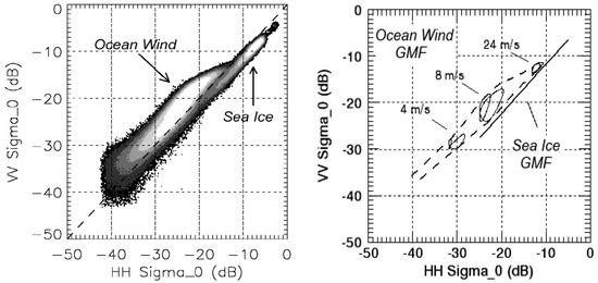
Figure 1.
Observed distribution of RCS (left) and empirical ocean wind and sea ice GMFs (right) in the space of QuikSCAT measurements [12].
To obtain quantitative characteristics of the reflecting surface, geophysical model functions (GMF) are used. For sea waves, the GMF depends on the wind speed and direction, the incidence angle, and the polarization of electromagnetic wave [13,14].
For the SeaWinds scatterometer on the QuikSCAT satellite, the GMF of sea ice is used the relationship between RCS at the vertical and horizontal polarizations [12]. It should be noted that measurements with the SeWinds scatterometer at vertical and horizontal polarizations are performed at different incidence angles.
In the ASCAT scatterometer, measurements are performed only on vertical polarization. When constructing the GMF, a regression analysis of the data accumulated at that moment is performed. In the future, the amount of data increases, so there is a need to refine the GMF based on a larger dataset. For example, for the ASCAT scatterometer, the fifth version of the GMF CMOD5 was developed in 2003 [15], and the seventh version of CMOD7 appeared in 2017 [16]. As a result, it is required to repeat the data processing.
At middle incidence angles, the problem is complicated by the fact that the RCS of the sea ice and sea waves are close in magnitude and the solution is ambiguous [17]. The use of two polarizations for the same incidence angles in a scatterometer is a promising direction [18,19].
The advantage of SAR over scatterometers is associated with a higher spatial resolution, which expands the range of problems to be solved. SAR performs measurements at different polarizations at the same incidence angle, which facilitates analysis. Figure 2 shows an example of using two polarizations to classify sea ice [20]. Another advantage of SAR is that it is possible to use not only co-polarizations, but also cross-polarization in processing algorithms, which increases the accuracy of the retrieval.
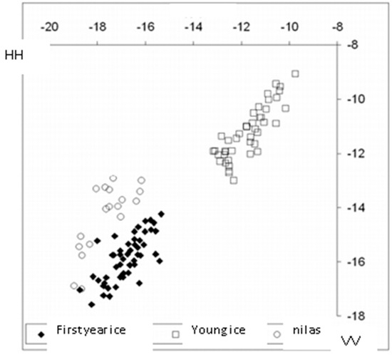
Figure 2.
RCS of various types of sea ice obtained from the Envisat satellite on horizontal and vertical polarizations [20].
At small incidence angles, the difference between the RCS of the sea ice and the sea waves is more significant, and for the wave scatterometer SWIM, which performs measurements at small incidence angles (<11°), an algorithm was developed, and completed validation confirmed its effectiveness [11].
However, from our point of view, the method that is based on the existing differences in the statistical characteristics of the sea ice and sea waves is more stable in processing. For example, at a positive air temperature, a thin layer of water (or wet ice) can form on the ice’s surface and the RCS will change when compared to the RCS of “dry” ice. A retrieval algorithm that uses the RCS as a criterion will give an error.
At the same time, the “roughness” of the sea ice and the sea waves is different. This is a reliable indicator of the type of scattering surface, as at small incidence angles, the RCS depends on the “roughness” of the surface. In this research, the “roughness” of the sea surface is understood as the mean square slopes () of a large scale, in comparison with the electromagnetic wavelength of sea waves. In what follows, we will use the short term: of large-scale sea waves or large-scale .
2. Measurement at the Small Incidence Angles
2.1. A Backscattered Radar Cross Section
The algorithm that uses the “roughness” of the scattering surface as a criterion was developed and used to analyze data from a Dual-frequency Precipitation Radar (DPR) [21,22]. Comparisons with radiometer data confirmed its effectiveness. Unlike existing retrieval algorithms, the new algorithm is not regressive and relies on the model of electromagnetic wave scattering by the sea waves at small incidence angles.
As is known, at small incidence angles, the quasi-specular backscattering mechanism is dominant, and the Kirchhoff method is used to calculate the reflected field [23,24,25,26]. With this approach, it is assumed that the main contribution to the reflected signal is made by sections of the wave profile oriented perpendicular to the incident electromagnetic wave.
In the Kirchhoff approximation, the equation for the RCS of sea waves has the following form [23]:
where and are the of large-scale sea waves along axis and axis , respectively; is the non-normalized correlation coefficient between the slopes along the axes and (hereinafter, the correlation coefficient); is the effective reflection coefficient introduced to take into account the influence of a short ripple on the power of the reflected signal [23,27].
For the sea surface, the distribution function of the of the large-scale sea waves is close to Gaussian; therefore, when the incidence angle changes along a fixed sounding direction, the dependence of the RCS on the incidence angle is also Gaussian. Examples of the dependence of the RCS on the incidence angle for the sea waves (left) and sea ice (right) are shown in Figure 3. The measurements were made with a DPR (Ku-band) and correspond to one scan in incidence angle (+/− 18 degrees) for sea ice (right) and sea waves (left). The figure is built on a linear scale and natural units (not dB).
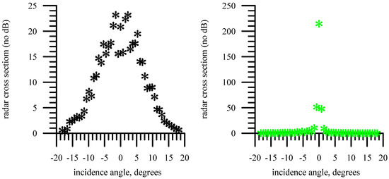
Figure 3.
Dependence of RCS on incidence angle for sea waves (left) and sea ice (right) in natural units (no dB). Step on the incidence angle is 0.7°.
It can be seen from the figure that the dependences of the RCS on the incidence angle of sea ice and sea waves are very different. This effect is independent of the value of RCS, so no radar calibration is required. One of the statistical characteristics that is commonly used in statistical analysis is the kurtosis coefficient, which is calculated as follows:
where —variance (the second central moment) and —the fourth central moment.
For a Gaussian dependence, the kurtosis coefficient is zero. If the kurtosis coefficient is different from zero, then this means that the reflection does not take place on the sea surface. Below we give brief information about the algorithm, which will be used in our calculations.
An example of a radar image of a precipitation radar obtained over the Sea of Okhotsk (top) and the result of calculating the kurtosis coefficient (bottom) is shown in Figure 4. The figure clearly shows a change in the structure of the radar image, which corresponds to a change in the underlying surface; there is a transition from ice cover (left) to sea waves (right).
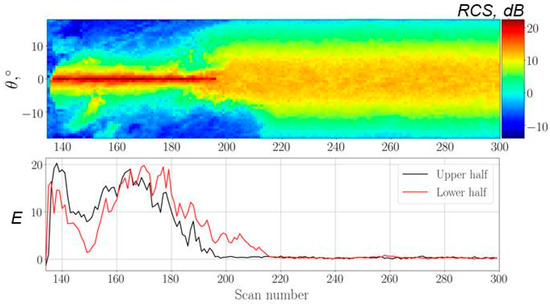
Figure 4.
Distribution of the RCS in the DPR swath (top) and kurtosis coefficient calculated for each corrected half of the scan (bottom). A red curve—right/lower half, a black curve—left/upper half.
During data processing, the swath was divided into two parts (to the left and to the right of the track). The resulting “halves” of the angular dependence were supplemented to the full and the kurtosis coefficient was calculated for them. This approach makes it possible to halve the length of the scan used for processing (improve spatial resolution).
The top figure shows the original radar image, and the bottom figure plots the kurtosis coefficients for the left/upper (black curve) and right/lower (red curve) parts of the radar image. The large-scale of sea waves is close to Gaussian, so the kurtosis coefficient decreases to zero when moving from the sea ice to the sea waves.
To illustrate the performance of the new algorithm based on the kurtosis coefficient, sea ice data retrieved from the AMSR-2 radiometer were used. Sea ice distribution according to Ku-band radar data on the GPM satellite (satellite orbit inclination is 65°–shown by red dotted line) for the first ten days of July 2018 and sea ice maps according to AMSR-2 radiometer data from the University of Bremen website for July 10, 2018 [28] are presented in Figure 5. Visual good agreement of the ice position for latitudes not higher than 65° according to the data of both instruments confirms the efficiency of the algorithm.
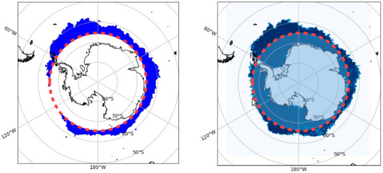
Figure 5.
The sea ice map according to DPR (left) and according to the University of Bremen (right) in Antarctica [28].
The disadvantage of the new algorithm is that the precipitation radar scans in a direction perpendicular to the direction of flight. As a result, the reflected signal is collected from an area approximately 120 km × 5 km in size, i.e., has insufficiently high spatial resolution for one of the coordinates, which will affect the accuracy of determining the sea ice boundary.
The accuracy estimate, possible limitations, and applicability criteria of the new algorithm are discussed in [21,22] and are beyond the scope of this research. Brief information about the algorithm is given in this paper in order to give an idea of the method that will be used to determine the type of scattering surface from the Doppler spectrum of the backscattered microwave radar signal.
2.2. A Doppler Spectrum
An alternative approach to determine the type of the scattering surface at small incidence angles is to measure the Doppler spectrum of the reflected microwave radar signal.
The Doppler spectrum of the reflected signal contains more information about the parameters of the sea surface compared to the RCS. The region of small incidence angles, when the Kirchhoff method is used to describe the reflected field, was considered separately. Theoretical models were developed and experiments were carried out to study the properties of Doppler spectra and numerical simulations were actively used, for example, in [29,30,31,32,33,34,35,36,37].
However, all Doppler spectrum models were related to the sea waves. In this study, we continue to consider the problem of applying the Doppler spectrum to detect sea ice [38,39]. For maximum accuracy, a wide or knife-like antenna beam should be used. Numerical simulation confirmed the effectiveness of the algorithm, which used the spectral characteristics of the reflected signal.
The numerical simulation was performed for a Doppler radar installed on an aircraft, i.e., for relatively a low flight altitude (<10 km) and a low speed (<300 m/s). For such a measurement scheme, even for a wide antenna pattern, the spatial resolution of the radar is high (a small footprint).
Comparison of the Doppler spectra reflected from the sea waves and the sea ice is shown in Figure 6 [38]. In this case, the difference in the Doppler spectra is also due to the difference in the roughness of the sea ice and the sea waves. From a mathematical point of view, this manifests itself in the difference in the scattering pattern of the surfaces or in the dependence of the backscattering RCS on the incidence angle for the reflecting surface.
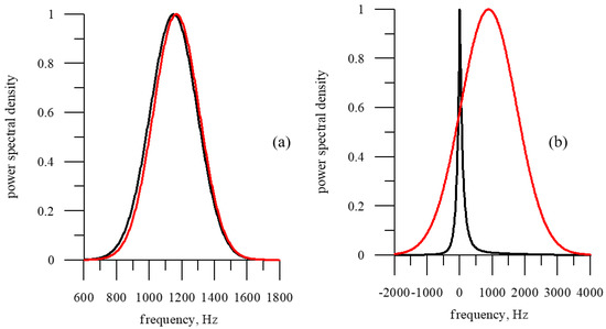
Figure 6.
Normalized Doppler spectra for a moving carrier ( = 200 m/s), incidence angle = 5°, azimuth angle = 45°, and two values of the antenna beam, 2° × 2° (a) and 14° × 2° (b): red curve—sea waves, and black curve—sea ice [38].
As can be seen from the figure, the use of the Doppler spectrum is an effective tool for determining the type of underlying surface. Installation of the microwave radar onto the satellite will degrade the spatial resolution and, hence, make the algorithm inefficient.
2.3. Advanced View of the Doppler Spectrum
In previous research, the option of installing a microwave radar with a knife-like antenna beam on the satellite was considered, and thanks to the developed original incoherent synthesis procedure, it is possible to significantly improve the spatial resolution and simulate (calculate) the backscattering RCS of a radar with a knife-like antenna beam for not an entire footprint but an elementary scattering cell [40,41,42].
In this paper the application of the proposed method (incoherent synthesis procedure) to the measured Doppler spectrum in order to improve the spatial resolution as applied to remote sensing of sea ice is discussed.
Figure 7 shows the measurement scheme. The radar moves along the axis at a height with a velocity . The sounding is carried out vertically downwards (incidence angle = 0°) and the knife-like antenna (1° × 20°) is oriented along the direction of motion. The following parameters are used in the calculations: an orbit altitude—500 km, a radar velocity—7 km/s.
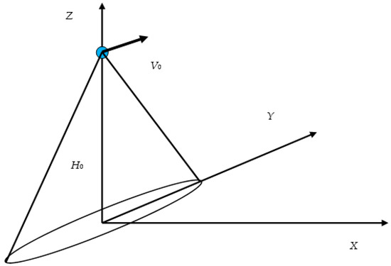
Figure 7.
Scheme of measurement.
With incidence angle = 0, the shift of the reflected Doppler spectrum will be zero, but the incidence angle varies within the antenna beam, so a width of Doppler spectrum will be large.
To calculate the reflected radar signal, it is necessary to know the surface scatterplot, and for the chosen measurement scheme, this is the dependence of the backscattering RCS on the incidence angle. In the general case, the RCS depends on the wind speed and direction relative to the direction of sounding, the length of the wind fetch, the parameters of swell for sea waves and on the characteristics of the sea ice and air temperature.
Based on the SWIM data, the GMF for the sea waves and sea ice at small incidence angles was developed for the first time [11] and the obtained dependences are shown in Figure 8.
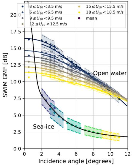
Figure 8.
Distribution of RCS over sea waves and sea ice as a function of incidence angle for SWIM. For the sea waves, the GMF is further detailed by wind speed [11].
The disadvantage of this data and GMF is that it cover a limited range of incidence angles (<11°) and therefore cannot be used for a wider or knife-like antenna beam.
It should be noted that this study did not aim to develop a ready-to-use algorithm, since there are currently no such radars in orbit. In this paper, we discuss a new method for determining (classifying) the type of scattering surface (sea ice–sea waves) from an orbital radar using the Doppler spectrum of the microwave signal. The capabilities of the new method are illustrated by numerical simulation, hence the choice of a particular GMF is not important for evaluating the capabilities of the method. Therefore, instead of the GMFs proposed in [11], we will use the GMFs, which cover a larger range of incidence angles [38,39].
In our research, we have used the Ku-band ( = 0.021 m) DPR data from the GPM satellite [9]. These data were used to determine the scatterplot of the underlying surface. As a result of the regression analysis, the dependence of RCS on incidence angle for the sea ice was approximated by the following Equation [38]:
where = −3.1518, = −0.008708, = −0.016928, = 26.013, = 0.5288 and incidence angle .
The dependence of the RCS on incidence angle for sea waves was approximated by the following Equation [38]:
where = 11.2912, = 0.00626, = −0.04076, = −0.000104, = 1.381 * 10−5, and = 7.911 * 10−8. To find the dependence, measurements of a DPR over the Sea of Okhotsk in the summer season averaged over several days were used.
On Figure 9 shows the dependences of the RCS on the incidence angle calculated by Equations (3) and (4). The red curve corresponds to the sea ice and the black curve to the sea waves. When plotting the figure, the RCS was converted to dB; therefore, in contrast to Figure 3, angular dependencies in this figure are clearly visible.
Figure 9.
Dependence of the RCS (GMF) on the incidence angle for sea ice (red curve) and sea waves (black curve).
The developed numerical model of the Doppler spectrum [38,39] was used to calculate the Doppler spectrum for the Doppler radar installed on the satellite. The procedure for modeling the Doppler spectrum is discussed in detail in the previous papers [38,39]. Figure 10 shows an example of a Doppler spectrum for an orbital radar (measurement scheme in Figure 7) for two cases: sea waves (dotted line) and sea ice (solid curve).
Figure 10.
Doppler spectrum measured by microwave radar mounted at the satellite: velocity—7 km/s; solid curve—sea ice; dashed line—sea waves. Incidence angle—0°, antenna beam—1° × 20°.
For the convenience of comparison of the Doppler spectra, they were normalized to the maxima. The antenna is oriented vertically downwards, so the shift of both Doppler spectra is zero. It is seen that the width of the Doppler spectrum for the sea waves is much wider than the Doppler spectrum for sea ice. This difference is due to the statistical properties of the reflecting surface, making the width of the Doppler spectrum a reliable indicator of the type of underlying surface.
In this research two extreme cases were considered: the sea ice concentration (SIC) was either 0 (sea waves) or 1 (sea ice). If the SIC of the sea ice is intermediate, then this will change the properties of the reflective surface and affect the Doppler spectrum. This is an interesting problem, but analysis of the effect of SIC was beyond the scope of this study.
3. New Methods
3.1. Radar Cross Section
At a permanent radar velocity, the Doppler shift of the backscattered radar signal depends on the incidence angle
where —radar wavelength; —incidence angle.
Therefore, the Doppler spectrum can be transformed into a dependence of the RCS on the incidence angle. The shape and parameters of the Doppler spectrum depend on the parameters of the antenna beam, so this will need to be taken into account during processing.
The algorithm for determining the type of scattering surface developed for DPR uses the dependence of the RCS on the incidence angle [21,22]. Angular dependence is formed as a result of scanning along the incidence angle with a narrow antenna beam (0.7° × 0.7°) and therefore the dependence of the RCS on the incidence angle is completely determined by the characteristics of the reflecting surface.
A radar with a knife-like antenna beam has a low spatial resolution. To improve it, the scattering area (footprint) can be divided into elementary scattering cells, as is done, for example, in scatterometry. On Figure 11 shows an example of splitting the SeaWinds scatterometer footprint into elementary scattering cells (slices) [43].
Figure 11.
The slices for a radar footprint [43].
When dividing a scattering area (footprint) formed by a wide or knife-like antenna beam into elementary scattering cells (slices), we obtained the dependence of the RCS on the incidence angle. However, it must be taken into account that the antenna beam will distort the form of the dependence and may be will not allow the use of a new algorithm that uses the kurtosis coefficient. Therefore, after transition from frequency to incidence angles, it is necessary to remove the dependence of the RCS on the antenna beam.
In the chosen measurement scheme (see Figure 7), all frequency changes are associated with a change in the incidence angle, which is counted from the zero incidence angle and this angle coincides with the angle inside the antenna beam.
In calculations, we assumed that the antenna beam is Gaussian, and is written in the following form:
where and are the antenna beam width at 0.5 power level along and axis; and are the incidence angle and azimuth angle within the antenna beam ().
For the chosen measurement scheme, the antenna beam is narrow (<<) and the change in the incidence angle along the axis can be neglected compared to the change in the incidence angle along the axis (azimuth angle) inside the antenna beam.
Remote sensing is performed at an incidence angle = 0°, and for a knife-like antenna, Equation (6) can be simplified and may be written as
Such a simplification is possible because, for the algorithm, the absolute values of RCS are not important, but the form of the angular dependence is important. In this case , therefore, further on, the angle will also be called the incidence angle.
As a result, in order to remove the influence of the antenna beam on the form of the dependence of RCS on incidence angle (), it is necessary to multiply the result by the function inverse to the antenna beam
An example of the transformation of the Doppler spectrum into the dependence of the RCS on the incidence angle is shown in Figure 12 for sea ice (left) and sea waves (right). The dotted line shows the initial dependence of the RCS on the incidence angle, and the solid curve shows the effects after removing the influence of the antenna beam. For ease of comparison, all dependences were normalized to the maximum.
Figure 12.
Dependence of the RCS on the incidence angle for sea ice (top) and sea waves (bottom): dotted curve—initial dependence; solid curve—corrected dependence (after removing the influence of antenna beam). All dependences were normalized to the maximum.
Consider the orientation of the antenna (1° × 20°) along the direction of flight. The Doppler spectrum corresponding to this case is shown in Figure 10. The Doppler spectrum was converted into a dependence of the RCS on the incidence angle, i.e., each backscattering RCS was assigned an incidence angle (see Figure 12).
With a flight altitude of 500 km and a width of the antenna beam of 20 degrees, the size of the scattering area (footprint) will be approximately 180 km at a power level of 0.5. The optimal width is 30°, however, in our numerical simulation, the maximum value of the antenna beam depends on the field of application of the GMF (see Equations (3) and (4)). In the case of such a large footprint, the calculated values of the RCS refer to different parts of the sea surface and, in the general case, sea waves or sea ice cannot be considered uniform over the entire scattering area (footprint).
To improve the spatial resolution and solve the problem of uniformity of the scattering surface, it is proposed to use an original approach that was developed for a knife-like microwave radar [40,41,42]. It was used to calculate the RCS.
The method consists of the scattering area (footprint) being divided into elementary scattering cells with a size, for example, 1° × 1°. In our numerical simulation, the backscattered signal is collected from an area along the axis of about 325 km.
The radar moves at a velocity of about 7 km/s, and during the time of flight across a footprint, which is about 46 s, each elementary scattering cell is observed at different incidence angles (see Figure 13a). Let us collect observations of an elementary cell at different incidence angles (see Figure 13b) and obtain the dependence of the RCS on the incidence angle for one elementary scattering cell.
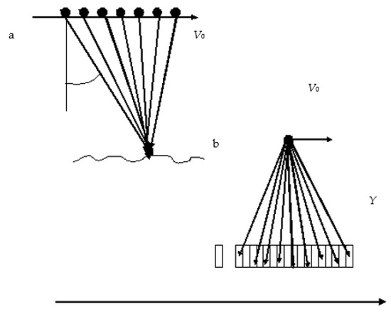
Figure 13.
Illustration of the incoherent synthesis procedure [41,42].
For an orbit altitude of 500 km, the elementary scattering cell size of 1° × 1° is approximately 9 × 9 km. For a cell of this size, sea waves (sea ice) can be considered homogeneous. Thus, using the original incoherent synthesis procedure, it is possible to obtain the dependence of the RCS on the incidence angle for one elementary scattering cell 9 × 9 km in size.
This can be interpreted as follows. The incoherent synthesis procedure forms from one elementary scattering cell with a “quasi–homogeneous” surface 325 km long (+/−18°), which consists of elementary cells that differ in time by about 1 s. The sea waves correlation time in the microwave range is less than 0.1 s [44,45], so all cells are uncorrelated, which reduces the effect of speckle noise on the result.
Thus, when using a Doppler microwave radar mounted on a satellite, it is possible to carry out measurements with high spatial resolution using a knife-like antenna beam oriented along the direction of flight.
Before consideration of the problem of classifying the type of the scattering surface according to the Doppler spectrum, let us consider an additional possibility of determining the characteristics of the reflecting surface. Previously, it was shown that the dependence of the RCS on the incidence angle can be used to determine the of large-scale sea waves, compared to the electromagnetic wavelength [46].
3.2. Numerical Simulation
There are no current microwave Doppler radars with knife-like antenna beams in orbit, so we ran numerical simulations to consistently demonstrate the operation of the new algorithm.
First of all, the Doppler spectra for the sea waves and sea ice were modeled (see Figure 10).
After that, with a step in the incidence angle 1°, the dependence of the RCS on the incidence angle was calculated (see Equation (5)). The result is shown in Figure 14 for sea ice (left) and sea waves (right).
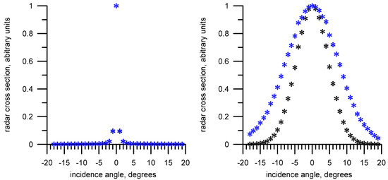
Figure 14.
Dependence of the RCS on the incidence angle for sea ice (left) and sea waves (right). Black asterisks correspond to the original dependence, and blue asterisks indicate removal of the dependence on the antenna beam.
For the sea waves, the angular dependence is smoother, so the influence of the antenna beam is clearly visible. For the sea ice, the angular dependence “drastically” drops, so the difference is not noticeable on a linear scale; the original and corrected dependences in the figure are not visually separated. To see it, you need to use the logarithmic scale (see Figure 12).
The last stage of the implementation of the algorithm is to calculate the kurtosis coefficient according to Equation (2). If the kurtosis coefficient is close to zero, then the reflection is from the sea waves. If more than one, then this is sea ice [21,22]. A detailed discussion of the criterion for separating sea ice and sea waves is given in [22].
3.3. Retrieval of of Large-Scale Sea Waves
To describe the reflection of electromagnetic waves by the sea surface at small incidence angles, the Kirchhoff method was used, and Equation (1) was used to calculate the RCS. The equation contains the along the sounding direction, therefore, having measurements for several incidence angles, it is possible to determine the of large-scale sea waves.
This is discussed in detail in [46,47]. In the simplest version, measurements of the two incidence angles are sufficient to calculate the . If we neglect the coefficient compared to the in Equation (1), then we obtain a simple equation for the of large-scale sea waves:
where and —incidence angles; and —RCS at these incidence angles.
The retrieved dependence of the backscattering RCS on the incidence angle (see Figure 14) makes it possible to use Equation (9) and estimate the of large-scale waves along the direction of sounding. For calculations, it is necessary to use corrected angular dependences, where there is no influence of the antenna beam.
4. Discussion
The simulation results show that the microwave Doppler radar is a promising tool for remote sensing, provided that a knife-like antenna beam is used [38,39]. When installing a radar on a satellite, the main problem is the low spatial resolution, which reduces the importance of the retrieved thematic information. The use of the original procedure of incoherent synthesis allows to significantly improve the spatial resolution and makes the information relevant. The information retrieved from the measured Doppler spectrum depends on the type of the scattering surface. The developed algorithms make it possible to determine the type of underlying surface (sea ice–sea waves) and, in the case of sea waves, the of large-scale waves was additionally determined.
Based on the experimental dependence of the RCS on the incidence angle for the sea waves (see Figure 9 and Equation (4)), which was used for modeling, the of large-scale sea waves along the sounding direction corresponding to this dependence was retrieved:
When processing, incidence angles are used in the range of 0–12 degrees, when the contribution of the Bragg scattering mechanism can be neglected. Some error in estimating the of large-scale sea waves is due to the fact that the dependence was built from experimental data collocated for a few days (DPR data).
To retrieve the of large-scale sea waves from the numerical simulation results, we used Figure 14, which shows the dependence of the RCS on the incidence angle for sea waves. Again, we take the angle interval of 0°–12° and calculate the from the original and corrected dependences using Equation (9).
Table 1 shows the results of processing the model data. The first column is the retrieved of large-scale sea waves.

Table 1.
Results of processing of model data.
The antenna beam reduces the RCS at the edges, which will be interpreted by the retrieval algorithm as a decrease in the of large-scale sea waves, since the angular dependence will become more steep (see “sea waves” (no corrected)—black asterisks, Figure 14). It can be seen from the table that the retrieved has decreased by more than two times compared to the correct value (see Equation (10)).
After correction (removal of the influence of the antenna beam–Equation (8)), the angular dependence becomes flatter (blue stars in Figure 14) and the is retrieved more accurately (see “sea waves” (corrected)). Thus, the removal of the effect of the antenna beam is a necessary step in the processing for retrieval.
The algorithm may be applied for sea waves, therefore, before applying it, it is necessary to determine the type of the scattering surface. To determine the type of underlying surface (sea ice–sea waves), it is necessary to calculate the kurtosis coefficient. The table shows the results of calculating the kurtosis coefficient for the sea waves and sea ice (see Figure 14).
The antenna beam distorts the dependence of the RCS on the incidence angle, making it narrower. This leads to an increase in the kurtosis coefficient. From a formal point of view, this improves the detection of sea ice.
This is due to the fact that the antenna beam is described by a Gaussian function (see Equation (6), so we get the multiplication of Gaussian functions, and the result will also be a Gaussian function, but narrower than the original ones. From the point of view of physics, this corresponds to a sea surface with a smaller . The processing results confirm this conclusion (see Table 1).
If the reflection is from sea ice, then the dependence of the RCS on the incidence angle is narrower than Gaussian function (large kurtosis). From the point of view of physics, the influence of the antenna is reduced to the multiplication of the angular dependence (no Gaussian function) by the Gaussian function. As a result, the RCS dependence on incidence becomes even narrower and the kurtosis coefficient increases, i.e., additional correction is not required to identify the underlying surface type.
In the research, two states of the sea surface were considered: sea waves and sea ice. An analysis of the situation when the SIC is less than one was beyond the scope of this study.
5. Conclusions
The monitoring of the sea ice area is an urgent task, and various equipment in the optical, IR, and microwave ranges are used to solve it. Placement of instruments on satellites allows obtaining global and operational information. Active radar has a number of advantages, and the development of new methods is an important task.
A study was made of the capabilities of an orbital microwave Doppler radar for classifying the type of scattering surface according to the ice/water criterion. It has been shown that orbital radar with knife-like antenna beam is sensitive to the “sea ice–sea waves” boundary, which makes it possible to estimate the area of sea ice. This is due to the fact that in the case of nadir sounding and orientation of the antenna beam along the direction of flight, the width of the Doppler spectrum depends on the “roughness” of the underlying surface. In this case, this is understood not as the height of roughness, but as the of large-scale sea waves. The criterion in the classification algorithm [21,22] is the kurtosis coefficient, which is equal to zero for the sea surface and can exceed 20–30 for the sea ice.
When placing a radar with a knife-like antenna beam in orbit, a serious problem arises with the size of the scattering area, in particular, with an orbit altitude of 500 km and an antenna beam width of 20° at a power level of 0.5, the footprint on the surface will be about 180 km (30–270 km).Moreover, inside the scattering area, the properties of the sea surface will not be uniform, which makes the algorithms inefficient for practical application.
To improve the spatial resolution, an original incoherent synthesis procedure was used, which made it possible to improve the resolution and retrieve the dependence of RCS on the incidence angle. Processing of the model data showed that sea waves and sea ice are confidently separated by the kurtosis coefficient.
During processing, it is possible to remove the dependence of the RCS on the antenna beam, which makes it possible to retrieve the slopes of large-scale sea waves along the sounding direction.
Thus, the orbital microwave Doppler radar is a promising tool for remote sensing of the sea surface.
For the first time, an experiment was carried out with a microwave Doppler radar installed on a technological trolley of a cable car. The measurements were taken while moving across the river in February (ice cover) and in September (water surface). Data processing will be performed to evaluate the effectiveness of the proposed approach.
Author Contributions
V.K. conceptualization and writing; Y.T. numerical simulation; M.P. writing–original draft preparation; K.P. software and numerical simulation; M.R. visualization; E.M. initiated the study; D.K. data processing. All authors have read and agreed to the published version of the manuscript.
Funding
This research was funded by Russian Science Foundation (project RSF 20–17–00179).
Data Availability Statement
Not applicable here.
Conflicts of Interest
The authors declare no conflict of interest.
References
- Anderson, H.; Long, D. Sea Ice mapping method for SeaWinds. IEEE Trans. Geosci. Remote Sens. 2005, 43, 647–657. [Google Scholar] [CrossRef]
- Fu, L.-L.; Cazenave, A. Satellite Altimetry and Earth Sciences; Academic Press: Cambridge, MA, USA, 2001. [Google Scholar]
- Zhang, Z.; Yu, Y.; Li, X.; Hui, F.; Cheng, X.; Chen, Z. Arctic sea ice classification using microwave scatterometer and radiometer data during 2002–2017. IEEE Trans. Geosci. Remote Sens. 2019, 57, 5319–5328. [Google Scholar] [CrossRef]
- Zakhatkina, N.Y.; Alexandrov, V.Y.; Johannessen, O.N.; Sandven, S.; Frolov, I.Y. Classification of sea ice types in ENVISAT synthetic aperture radar images. IEEE Trans. Geosci. Remote Sens. 2013, 51, 2587–2600. [Google Scholar] [CrossRef]
- Komarov, A.; Buehner, M. Detection of first-year and multi-year ice from dual-polarization SAR images under cold conditions. IEEE Trans. Geosci. Remote Sens. 2019, 57, 9109–9123. [Google Scholar] [CrossRef]
- Leigh, S.; Wing, Z.; Clausi, D. Automated ice-water classification using dual polarization SAR satellite imagery. IEEE Trans. Geosci. Remote Sens. 2014, 52, 5529–5539. [Google Scholar] [CrossRef]
- Cooke, C.; Scott, A. Estimating sea ica concentration from SAR: Training convolutional neural networks with passive microwave data. IEEE Trans. Geosci. Remote Sens. 2019, 57, 4735–4747. [Google Scholar] [CrossRef]
- NASDA. TRMM Data Users Handbook; NASDA: Arlington, VA, USA, 2001; p. 226. [Google Scholar]
- JAXA. GPM Data Utilization Handbook, 1st ed.; JAXA: Tokyo, Japan, 2014; p. 92. [Google Scholar]
- Hauser, D.; Tison, C.; Amiot, T.; Delaye, L.; Corcoral, N.; Castillan, P. SWIM: The First Spaceborne Wave Scatterometer. Trans. Geosci. Remote Sens. 2017, 55, 3000–3014. [Google Scholar] [CrossRef]
- Peureux, C.; Longepe, N.; Mouche, A.; Tison, C.; Tourain, C.; Lachiver, J.-M.; Hauser, D. Sea-ice detection from near-nadir Ku-band echoes from CFOSAT/SWIM scatterometer. Earth Space Sci. 2022. [Google Scholar] [CrossRef]
- Rivas, M.B.; Stoffelen, A. New Bayesian algorithm for sea ice detection with Quikscat. IEEE Trans. Geosci. Remote Sens. 2011, 49, 1894–1901. [Google Scholar] [CrossRef]
- Stoffelen, A.; Anderson, D. The ECMWF Contribution to the Characterization, Interpretation, Calibration and Validation of ERS-1 Scatterometer Backscatter Measurements and Their Use in Numerical Weather Prediction Models; ECMWF Contract Report 9097/90/NL/BI; ECMWF: Shinfield Park, UK, 1995; 92p. [Google Scholar]
- Wentz, F.J.; Smith D., K. A model function for the ocean-normalized radar cross section at 14 GHz derived from NSCAT observations. J. Geophys. Res. 1999, 104, 11499–11514. [Google Scholar] [CrossRef]
- Hersbach, H.; Stoffelen, A.; Haan, S. An improved C-band scatterometer ocean geophysical model function: CMOD5. J. Geophys. Res. 2007, 112, C03006. [Google Scholar] [CrossRef]
- Stoffelen, A.; Verspeek J., A.; Vogelzang, J.; Verhoef, A. The CMOD7 geophysical model function for ASCAT and ERS wind retrievals. IEEE J. Sel. Top. Appl. Earth Obs. Remote Sens. 2017, 10, 2123–2134. [Google Scholar] [CrossRef]
- Murtazin, A.; Efgrafova, K.; Kudryavtsev, V. Application of ASCAT scatterometer data to study the ice cover in the Arctic. Uchenye Zap. Ross. Gos. Gidrol. Univ. 2015, 40, 160–173. (In Russian) [Google Scholar]
- Nekrasov, A.; Khachaturian, A.; Labun, J.; Kurdel, P.; Bogachev, M. Towards the sea ice and wind measurement by a C-band scatterometer at dual VV/HH polarization: A prospective appraisal. Remote Sens. 2020, 12, 3382. [Google Scholar] [CrossRef]
- Rivas, M.; Stoffelen, A.; Zadelhoff, G.-J. The Benefit of HH and VH Polarizations in Retrieving Extreme Wind Speeds for an ASCAT-Type Scatterometer. IEEE Trans. Geosci. Remote Sens. 2014, 52, 4273–4280. [Google Scholar] [CrossRef]
- Alexandrov, V. Satellite Radar Monitoring of Sea Ice Cover. Ph.D. Thesis, Nansen International Center for Environment and Remote Sensing—“Nansen Center”, Sankt-Petersburg, Russia, 2010; p. 349. [Google Scholar]
- Panfilova, M.; Shikov, S.; Karaev, V. Sea ice detection using Ku-band onboard GPM satellite. In Proceedings of the URSI GASS 2020, Rome, Italy, 29 August–5 September 2020. [Google Scholar] [CrossRef]
- Panfilova, M. Retrieval of Sea Wave Parameters, Wind Speed and Sea Ice Cover Position from Remote Sensing Data in the Microwave Range at Small Incidence Angles. Ph.D. Thesis, Institute of Applied Physics RAS, Nizhny Novgorod, Russia, 2022; p. 112. (In Russian). [Google Scholar]
- Bass, F.G.; Fuks, I.M. Scattering of Waves by Statistically Rough Surfaces; Pergamon Press: Oxford, UK, 1979; p. 528. [Google Scholar]
- Barrick, D.E. Rough surface scattering based on the specular point theory. IEEE Trans. AP-16 1968, 16, 449–554. [Google Scholar] [CrossRef]
- Valenzuela, G. Theories for the interaction of electromagnetic and oceanic waves—A review. Bound. Layer Meteorol. 1978, 13, 61–86. [Google Scholar] [CrossRef]
- Isakovich, M.A. Scattering of waves from a statistically rough surface. J. Theor. Exp. Phys. 1952, 23, 305–314. (In Russian) [Google Scholar]
- Freilich, M.; Vanhoff, B. The relationship between winds, surface roughness, and radar backscatter at low incidence angles from TRMM precipitation radar measurements. J. Atmos. Ocean. Technol. 2003, 20, 549–562. [Google Scholar] [CrossRef]
- Sea ice Remote Sensing. Available online: https://seaice.uni-bremen.de/start/ (accessed on 1 August 2022).
- Thompson, D.R. Calculation of microwave Doppler spectra from the ocean surface with a time-dependent composite model. In Radar Scattering from Modulated Wind Waves; Komen, J., Oost, W., Eds.; Kluwer Academic Publisher: Philip Drive Norwell, MA, USA, 1989; pp. 27–40. [Google Scholar] [CrossRef]
- Fois, F.; Hoogeboom, P.; Chevalier, F.L.; Stoffelen, A. An analytical model for the description of the full polarimetric sea surface Doppler signature. J. Geophys. Res. Ocean. 2015, 120, 988–1015. [Google Scholar] [CrossRef]
- Nouguier, F.; Guerin, C.; Soriano, G. Analytical techniques for the Doppler signature of sea surfaces in the microwave regime-I: Linear surfaces. IEEE Trans. Geosci. Remote Sens. 2011, 49, 4856–4864. [Google Scholar] [CrossRef]
- Nouguier, F.; Guerin, C.; Soriano, G. Analytical techniques for the Doppler signature of sea surfaces in the microwave regime-II: Nonlinear surfaces. IEEE Trans. Geosci. Remote Sens. 2011, 49, 4920–4927. [Google Scholar] [CrossRef]
- Wang, Y.; Zhang, Y.; Li, H.; Chen, G. Doppler spectrum of microwave SAR signals from two-dimensional time-varying sea surface. J. Electromagn. Waves Appl. 2016, 30, 1265–1276. [Google Scholar] [CrossRef]
- Toporkov, J.; Sletten, M.; Brown, G. Numerical scattering simulations from time-evolving ocean-like surfaces at L- and X-band: Doppler analysis and comparisons with a composite surface analytical model. In Proceedings of the XXVII URSI General Assembly, Maastricht, The Netherlands, 17–24 August 2002. [Google Scholar]
- Toporkov, J.V.; Brown, G. Numerical simulations of scattering from time varying, randomly rough surfaces. IEEE Trans. Geosci. Remote Sens. 2000, 38, 1616–1625. [Google Scholar] [CrossRef]
- Li, X.; Xu, X. Scattering and Doppler spectral analysis for two-dimensional linear and nonlinear sea surfaces. IEEE Trans. Geosci. Remote Sens. 2011, 49, 603–611. [Google Scholar] [CrossRef]
- Yurovsky, Y.; Kudryavtsev, V.; A. Grodsky, S.; Chapron, B. Sea Surface Ka-Band Doppler Measurements: Analysis and Model Development. Remote Sens. 2019, 11, 839. [Google Scholar] [CrossRef]
- Karaev, V.; Titchenko, Y.; Panfilova, M.; Ryabkova, M.; Meshkov, E.; Ponur, K. Application of the Doppler spectrum of the backscattering microwave signal for monitoring of ice cover: A theoretical view. Remote Sens. 2022, 14, 2331. [Google Scholar] [CrossRef]
- Karaev, V.; Titchenko, Y.; Panfilova, M.; Ryabkova, M.; Meshkov, E.; Ponur, K. Doppler spectrum as the perspective instrument for detection of the ice cover. In Proceedings of the IGARSS, Kuala Lumpur, Malaysia, 17–22 July 2022; 2022; pp. 3919–3922. [Google Scholar]
- Karaev, V.; Kanevsky, M.; Meshkov, E.; Kovalenko, A. The concept of the scanning radar with knife-like beam for remote sensing of the ocean at small incidence angles. In Proceedings of the 4th Coastal altimetry Workshop, Porto, Portugal, 14–15 October 2010. [Google Scholar]
- Karaev, V.; Kanevsky, M.; Balandina, G.; Meshkov, E.; Challenor, P.; Srokosz, M.; Gommenginger, C. A rotating knife-beam altimeter for wide-swath remote sensing of the ocean: Wind and waves. Sensors 2006, 6, 260–281. [Google Scholar] [CrossRef]
- Karaev, V.; Kanevsky, M.; Balandina, G.; Challenor, P.; Gommenginger, C.; Srokosz, M. The concept of a microwave radar with asymmetric knife-like beam for the remote sensing of Ocean Waves. J. Atmos. Ocean. Technol. 2005, 22, 1809–1820. [Google Scholar] [CrossRef]
- Portabella, M. Wind Field Retrieval from Satellite Radar Systems. Ph.D. Thesis, University of Barcelona, Barcelona, Spain, 2002; p. 206. [Google Scholar]
- Winebrenner, D.; Hasselman, K. Specular point scattering contribution to the mean synthetic aperture radar image of the ocean. J. Geophys. Res. 1988, 93, 9281-92-94. [Google Scholar] [CrossRef]
- Bass, F.; Razskazovsky, V.; Andreenko, N.; Egorova, L.; Kivva, F.; Kostenko, A.; Kulemin, G.; Shestopalov, V. Radiophysical Researches of the World Ocean; Institute of Radiophysics and Electronics of the Academy of Sciences of Ukraine: Kharkov, Ukraine, 1992; 220p. [Google Scholar]
- Panfilova, M.; Karaev, V.; Mitnik, L.; Titchenko, Y.; Ryabkova, M.; Meshkov, E. Andvanced view at the Ocean Surface. J. Geophys. Researh Ocean. 2020, 125, e2020JC016531. [Google Scholar] [CrossRef]
- Li, X.; Karaev, V.; Panfilova, M.; Liu, B.; Wang, Z.; Xu, Y.; Liu, J.; He, Y. Measurements of total sea surface mean square slope field based on SWIM data. IEEE Trans. Geosci. Remote Sens. 2022, 60, 1–9. [Google Scholar] [CrossRef]
Publisher’s Note: MDPI stays neutral with regard to jurisdictional claims in published maps and institutional affiliations. |
© 2022 by the authors. Licensee MDPI, Basel, Switzerland. This article is an open access article distributed under the terms and conditions of the Creative Commons Attribution (CC BY) license (https://creativecommons.org/licenses/by/4.0/).