


Retrieval of Chlorophyll-a Concentrations Using Sentinel-2 MSI Imagery in Lake Chagan Based on Assessments with Machine Learning Models


Abstract
1. Introduction
2. Study Area and Data
2.1. Study Area
2.2. In-Situ Data Collection
2.3. Satellite Data
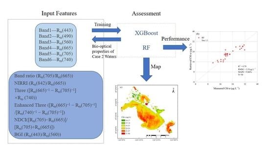
3. Methodology
3.1. Model Structure

| Algorithm | Index | Reference |
|---|---|---|
| Band ratio | Rrs(709)/Rrs(665) | Duan et al. [20] |
| Three | [Rrs(671)−1 − Rrs(710)−1] × Rrs(740) | Gitelson et al. [21] |
| Enhanced Three | [Rrs (665)−1 − Rrs(705)−1]/ [Rrs (740)−1 − Rrs(705)−1] | Yang et al. [23] |
| NIRRI | Rrs(865)/Rrs(655) | Duan et al. [13] |
| NDCI | [Rrs (708)−1 − Rrs(665)−1]/ [Rrs (708)−1 + Rrs(665)−1] | Mishra et al. [40] |
| BGI | Rrs(443)/Rrs(561) | Nguyen et al. [41] |
3.2. SHAP Method
3.3. KNN for the Seasonal Pattern Test
3.4. Accuracy Assessment
4. Results
4.1. Development and Assessment of the Models
4.1.1. Performance of XGBoost and RF
4.1.2. Assessment through SHAP
4.2. Spatial and Temporal Analysis of Chl-a
4.2.1. Test for Seasonal Patterns of Chl-a Concentrations
4.2.2. Robustness Analysis of RF in Three Seasons
4.2.3. Seasonal and Spatial Analysis
5. Discussion
5.1. Significance of the Input Features in ML
5.2. Comparison with Other Empirical Algorithms
5.3. Validation of In Situ and Sentinel-2 Reflectance
5.4. Ecological Variations across Lakes between 2020 and 2021
6. Conclusions
Author Contributions
Funding
Data Availability Statement
Conflicts of Interest
References
- Jian, J.; Bailey, V.; Dorheim, K.; Konings, A.G.; Hao, D.; Shiklomanov, A.N.; Snyder, A.; Steele, M.; Teramoto, M.; Vargas, R.; et al. Historically inconsistent productivity and respiration fluxes in the global terrestrial carbon cycle. Nat. Commun. 2022, 13, 1–9. [Google Scholar] [CrossRef]
- Qiu, R.; Li, X.; Han, G.; Xiao, J.; Ma, X.; Gong, W. Monitoring drought impacts on crop productivity of the US Midwest with solar-induced fluorescence: GOSIF outperforms GOME-2 SIF and MODIS NDVI, EVI, and NIRv. Agric. For. Meteorol. 2022, 323, 109038. [Google Scholar] [CrossRef]
- Li, Y.; Ma, Q.; Chen, J.M.; Croft, H.; Luo, X.; Zheng, T.; Rogers, C.; Liu, J. Fine-scale leaf chlorophyll distribution across a deciduous forest through two-step model inversion from Sentinel-2 data. Remote Sens. Environ. 2021, 264, 112618. [Google Scholar] [CrossRef]
- Brooks, B.W.; Lazorchak, J.M.; Howard, M.D.; Johnson, M.V.; Morton, S.L.; Perkins, D.A.; Reavie, E.D.; Scott, G.I.; Smith, S.A.; Steevens, J.A. Are harmful algal blooms becoming the greatest inland water quality threat to public health and aquatic ecosystems? Environ. Toxicol. Chem. 2016, 35, 6–13. [Google Scholar] [CrossRef]
- Mansaray, A.S.; Dzialowski, A.R.; Martin, M.E.; Wagner, K.L.; Stoodley, S.H. Comparing PlanetScope to Landsat-8 and Sentinel-2 for Sensing Water Quality in Reservoirs in Agricultural Watersheds. Remote Sens. 2021, 13, 1847. [Google Scholar] [CrossRef]
- OReilly, J.E.; Werdell, P.J. Chlorophyll algorithms for ocean color sensors—OC4, OC5 & OC6. Remote Sens. Environ. 2019, 229, 32–47. [Google Scholar]
- Antoine, D.; André, J.M.; Morel, A. Oceanic primary production: 2. Estimation at global scale from satellite (coastal zone color scanner) chlorophyll. Global Bio-Geochem. Cycl. 1996, 10, 57–69. [Google Scholar] [CrossRef]
- OReilly, J.E.; Maritorena, S.; Mitchell, B.G.; Siegel, D.A.; Carder, K.L.; Garver, S.A.; Kahru, M.; McClain, C. Ocean color chlorophyll algorithms for SeaWiFS. J. Geophys. Res. Ocean 1998, 103, 24937. [Google Scholar] [CrossRef]
- Chen, Z.; Hu, C.; Conmy, R.N.; Muller-Karger, F.; Swarzenski, P. Colored dissolved organic matter in Tampa Bay, Florida. Mar. Chem. 2007, 104, 98–109. [Google Scholar] [CrossRef]
- Hang, X.; Li, Y.; Li, X.; Meng, X.; Sun, L. Estimation of Chlorophyll-a Concentration in Lake Taihu from Gaofen-1 Wide-Field-of-View Data through a Machine Learning Trained Algorithm. J. Meteorol. Res. 2022, 36, 208–226. [Google Scholar] [CrossRef]
- Pahlevan, N.; Smith, B.; Schalles, J.; Binding, C.E.; Cao, Z.; Ma, R.; Alikas, K.; Kangro, K.; Gurlin, D.; Hà, N.; et al. Seamless retrievals of chlorophyll-a from Sentinel-2 (MSI) and Sentinel-3 (OLCI) in inland and coastal waters: A machine-learning approach. Remote Sens. Environ. 2020, 240, 111604. [Google Scholar] [CrossRef]
- Gregg, W.W.; Casey, N.W. Sampling biases in MODIS and SeaWiFS ocean chlorophyll data. Remote Sens. Environ. 2007, 111, 25–35. [Google Scholar] [CrossRef]
- Duan, H.; Zhang, Y.; Zhang, B.; Song, K.; Wang, Z. Assessment of chlorophyll-a concentration and trophic state for Lake Chagan using Landsat TM and field spectral data. Environ. Monit. Assess 2007, 129, 295–308. [Google Scholar] [CrossRef] [PubMed]
- Bonansea, M.; Rodriguez, M.C.; Pinotti, L.; Ferrero, S. Using multi-temporal Landsat imagery and linear mixed models for assessing water quality parameters in Río Tercero reservoir (Argentina). Remote Sens. Environ. 2015, 158, 28–41. [Google Scholar] [CrossRef]
- Cao, Z.; Ma, R.; Duan, H.; Pahlevan, N.; Melack, J.; Shen, M.; Xue, K. A machine learning approach to estimate chlorophyll-a from Landsat-8 measurements in inland lakes. Remote Sens. Environ. 2020, 248, 111974. [Google Scholar] [CrossRef]
- Toming, K.; Kutser, T.; Laas, A.; Sepp, M.; Paavel, B.; Nõges, T. First experiences in mapping lake water quality parameters with Sentinel-2 MSI imagery. Remote Sens. 2016, 8, 640. [Google Scholar] [CrossRef]
- Buma, W.G.; Lee, S.I. Evaluation of sentinel-2 and landsat 8 images for estimating chlorophyll-a concentrations in lake Chad, Africa. Remote Sens. 2020, 12, 2437. [Google Scholar] [CrossRef]
- Li, J.; Ma, R.; Xue, K.; Zhang, Y.; Loiselle, S. A remote sensing algorithm of column-integrated algal biomass covering algal bloom conditions in a shallow Eutrophic Lake. ISPRS Int. J. Geo-Inf. 2018, 7, 466. [Google Scholar] [CrossRef]
- Lyu, H.; Li, X.; Wang, Y.; Jin, Q.; Cao, K.; Wang, Q.; Li, Y. Evaluation of chlorophyll-a retrieval algorithms based on MERIS bands for optically varying eutrophic inland lakes. Sci. Total Environ. 2015, 530, 373–382. [Google Scholar] [CrossRef] [PubMed]
- Duan, H.; Ma, R.; Hu, C. Evaluation of remote sensing algorithms for cyanobacterial pigment retrievals during spring bloom formation in several lakes of East China. Remote Sens. Environ. 2012, 126, 126–135. [Google Scholar] [CrossRef]
- Gitelson, A.A.; Gao, B.C.; Li, R.R.; Berdnikov, S.; Saprygin, V. Estimation of chlorophyll-a concentration in productive turbid waters using a Hyperspectral Imager for the Coastal Ocean—The Azov Sea case study. Environ. Res. Lett. 2011, 6, 024023. [Google Scholar] [CrossRef]
- Le, C.; Hu, C.; Cannizzaro, J.; English, D.; Muller-Karger, F.; Lee, Z. Evaluation of chlorophyll-a remote sensing algorithms for an optically complex estuary. Remote Sens. Environ. 2013, 129, 75–89. [Google Scholar] [CrossRef]
- Yang, W.; Matsushita, B.; Chen, J.; Fukushima, T.; Ma, R. An enhanced three-band index for estimating chlorophyll-a in turbid case-II waters: Case studies of Lake Kasumigaura, Japan, and Lake Dianchi, China. IEEE Trans. Geosci. Remote Sens. Lett. 2010, 7, 655–659. [Google Scholar] [CrossRef]
- Li, S.; Song, K.; Wang, S.; Liu, G.; Wen, Z.; Shang, Y.; Lyu, L.; Chen, F.; Xu, S.; Tao, H.; et al. Quantification of chlorophyll-a in typical lakes across China using Sentinel-2 MSI imagery with machine learning algorithm. Sci. Total Environ. 2021, 778, 146271. [Google Scholar] [CrossRef]
- Kwon, Y.S.; Baek, S.H.; Lim, Y.K.; Pyo, J.; Ligaray, M.; Park, Y.; Cho, K.H. Monitoring coastal chlorophyll-a concentrations in coastal areas using machine learning models. Water 2018, 10, 1020. [Google Scholar] [CrossRef]
- Topp, S.N.; Pavelsky, T.M.; Jensen, D.; Simard, M.; Ross, M.R. Research trends in the use of remote sensing for inland water quality science: Moving towards multidisciplinary applications. Water 2020, 12, 169. [Google Scholar] [CrossRef]
- Hafeez, S.; Wong, M.S.; Ho, H.C.; Nazeer, M.; Nichol, J.; Abbas, S.; Tang, D.; Lee, K.H.; Pun, L. Comparison of machine learning algorithms for retrieval of water quality indicators in case-II waters: A case study of Hong Kong. Remote Sens. 2019, 11, 617. [Google Scholar] [CrossRef]
- Yang, H.; Du, Y.; Zhao, H.; Chen, F. Water Quality Chl-a Inversion Based on Spatio-Temporal Fusion and Convolutional Neural Network. Remote Sens. 2022, 14, 1267. [Google Scholar] [CrossRef]
- Liu, T.; Gu, Y.; Jia, X. Class-guided coupled dictionary learning for multispectral-hyperspectral remote sensing image collaborative classification. Sci. China Technol. Sci. 2022, 65, 744–758. [Google Scholar] [CrossRef]
- Cui, Y.; Meng, F.; Fu, P.; Yang, X.; Zhang, Y.; Liu, P. Application of hyperspectral analysis of chlorophyll a concentration inversion in Nansi Lake. Ecol. Inform. 2021, 64, 101360. [Google Scholar] [CrossRef]
- Lundberg, S.M.; Lee, S.I. A unified approach to interpreting model predictions. Proc. Adv. Neural Inf. Process. Syst. 2017, 30, 1–10. [Google Scholar]
- Lundberg, S.M.; Erion, G.; Chen, H.; DeGrave, A.; Prutkin, J.M.; Nair, B.; Katz, R.; Himmelfarb, J.; Bansal, N.; Lee, S.I. From local explanations to global understanding with explainable AI for trees. Nat. Mach. Intell. 2020, 2, 56–67. [Google Scholar] [CrossRef]
- Kim, Y.W.; Kim, T.; Shin, J.; Lee, D.S.; Park, Y.S.; Kim, Y.; Cha, Y. Validity evaluation of a machine-learning model for chlorophyll a retrieval using Sentinel-2 from inland and coastal waters. Ecol. Indicat. 2022, 137, 108737. [Google Scholar] [CrossRef]
- Zhu, L.; Yan, B.; Wang, L.; Pan, X. Mercury concentration in the muscle of seven fish species from Chagan Lake, Northeast China. Environ. Monit. Assess 2012, 184, 1299–1310. [Google Scholar] [CrossRef]
- Mobley, C.D. Estimation of the remote-sensing reflectance from above-surface measurements. Appl. Opt. 1999, 38, 7442–7455. [Google Scholar] [CrossRef] [PubMed]
- Gascon, F.; Bouzinac, C.; Thépaut, O.; Jung, M.; Francesconi, B.; Louis, J.; Lonjou, V.; Lafrance, B.; Massera, S.; Gaudel-Vacaresse, A.; et al. Copernicus Sentinel-2A calibration and products validation status. Remote Sens. 2017, 9, 584. [Google Scholar] [CrossRef]
- Rodríguez-Pérez, R.; Bajorath, J. Interpretation of compound activity predictions from complex machine learning models using local approximations and shapley values. J. Med. Chem. 2019, 63, 8761–8777. [Google Scholar] [CrossRef]
- Park, J.; Lee, W.H.; Kim, K.T.; Park, C.Y.; Lee, S.; Heo, T.Y. Interpretation of ensemble learning to predict water quality using explainable artificial intelligence. Sci. Total Environ. 2022, 832, 155070. [Google Scholar] [CrossRef]
- Breiman, L. Random forests. Mach. Learn. 2001, 45, 5–32. [Google Scholar] [CrossRef]
- Mishra, S.; Mishra, D.R. Normalized difference chlorophyll index: A novel model for remote estimation of chlorophyll-a concentration in turbid productive waters. Remote Sens. Environ. 2012, 117, 394–406. [Google Scholar] [CrossRef]
- Ha, N.T.; Koike, K.; Nhuan, M.T.; Canh, B.D.; Thao, N.T.; Parsons, M. Landsat 8/OLI two bands ratio algorithm for chlorophyll-a concentration mapping in hypertrophic waters: An application to West Lake in Hanoi (Vietnam). IEEE J. Select. Top. Appl. Earth Observat. Remote Sens. 2017, 10, 4919–4929. [Google Scholar] [CrossRef]
- Cover, T.; Hart, P. Nearest neighbour pattern classification. IEEE Trans. Inf. Theory 1967, 13, 21–27. [Google Scholar] [CrossRef]
- Hwang, W.J.; Wen, K.W. Fast kNN classification algorithm based on partial distance search. Electron. Lett. 1998, 34, 2062–2063. [Google Scholar] [CrossRef]
- Lee, Z.P.; Carder, K.L.; Peacock, T.G.; Davis, C.O.; Mueller, J.L. Method to derive ocean absorption coefficients from remote-sensing reflectance. Appl. Opt. 1996, 35, 453–462. [Google Scholar] [CrossRef]
- Chicco, D.; Jurman, G. The advantages of the Matthews correlation coefficient (MCC) over F1 score and accuracy in binary classification evaluation. BMC Genom. 2020, 21, 1–13. [Google Scholar] [CrossRef]
- Zhang, S. Cost-sensitive KNN classification. Neurocomputing 2020, 391, 234–242. [Google Scholar] [CrossRef]
- Shi, K.; Zhang, Y.; Xu, H.; Zhu, G.; Qin, B.; Huang, C.; Liu, X.; Zhou, Y.; Lv, H. Long-term satellite observations of microcystin concentrations in Lake Taihu during cyanobacterial bloom periods. Environ. Sci. Technol. 2015, 49, 6448–6456. [Google Scholar] [CrossRef] [PubMed]
- Ciancia, E.; Magalhães Loureiro, C.; Mendonça, A.; Coviello, I.; Di Polito, C.; Lacava, T.; Pergola, N.; Satriano, V.; Tramutoli, V.; Martins, A. On the potential of an RST-based analysis of the MODIS-derived chl-a product over Condor seamount and surrounding areas (Azores, NE Atlantic). Ocean Dyn. 2016, 66, 1165–1180. [Google Scholar] [CrossRef]
- Odermatt, D.; Gitelson, A.; Brando, V.E.; Schaepman, M. Review of constituent retrieval in optically deep and complex waters from satellite imagery. Remote Sens. Environ. 2012, 118, 116–126. [Google Scholar] [CrossRef]
- Friedman, J.H. Greedy Function Approximation: A Gradient Boosting Machine. Ann. Statist. 2001, 29, 1189–1232. [Google Scholar] [CrossRef]
- Downing, J.A.; Prairie, Y.T.; Cole, J.J.; Duarte, C.M.; Tranvik, L.J.; Striegl, R.G.; McDowell, W.H.; Kortelainen, P.; Caraco, N.F.; Melack, J.M.; et al. The global abundance and size distribution of lakes, ponds, and impoundments. Limnol. Oceanogr. 2006, 51, 2388–2397. [Google Scholar] [CrossRef]
- Nguyen, H.Q.; Ha, N.T.; Nguyen-Ngoc, L.; Pham, T.L. Comparing the performance of machine learning algorithms for remote and in situ estimations of chlorophyll-a content: A case study in the Tri An Reservoir, Vietnam. Water Environ. Res. 2021, 93, 2941–2957. [Google Scholar] [CrossRef]
- Li, S.; Song, K.; Zhao, Y.; Mu, G.; Shao, T.; Ma, J. Absorption characteristics of particulates and CDOM in waters of Chagan Lake and Xinlicheng Reservoir in autumn. Huan Jing Ke Xue 2016, 37, 112–122. [Google Scholar] [PubMed]
- Feng, L.; Hu, C.; Chen, X.; Zhao, X. Dramatic inundation changes of China’s two largest freshwater lakes linked to the Three Gorges Dam. Environ. Sci. Technol. 2013, 47, 9628–9634. [Google Scholar] [CrossRef] [PubMed]


| In-Situ Date | Number of Points | Average (μg L−1) |
|---|---|---|
| 22 July 2020 | 20 | 20.78 |
| 21 August 2020 | 18 | 19.61 |
| 26 September 2020 | 20 | 24.46 |
| 26 May 2021 | 20 | 15.60 |
| 18 July 2021 | 20 | 28.47 |
| Sentinel-2 Bands | Central Wavelength (nm) | Resolution (m) |
|---|---|---|
| Band 1—Coastal aerosol | 443 | 60 |
| Band 2—Blue | 490 | 10 |
| Band3—Green | 560 | 10 |
| Band 4—Red | 665 | 10 |
| Band 5—Vegetation red edge | 705 | 20 |
| Band 6—Vegetation red edge | 740 | 20 |
| Band 8—NIR | 842 | 10 |
| Year | In-Situ Date | Sentinel-2 Date |
|---|---|---|
| 2020 | 22 July | 22 July |
| 2020 | 21 August | 21 August |
| 2020 | 26 September | 30 September |
| 2021 | 26 May | 18 May |
| 2021 | 18 July | 22 July |
| Model | R2 | RMSE (μg L−1) | MAPE (%) |
|---|---|---|---|
| RF-3 features | 0.71 | 2.91 | 11.41 |
| RF-4 features | 0.75 | 2.74 | 10.63 |
| RF-5 features | 0.75 | 2.71 | 10.81 |
| RF-6 features | 0.72 | 2.90 | 11.08 |
| RF-7 features | 0.73 | 2.83 | 10.87 |
| RF-8 features | 0.70 | 2.99 | 11.27 |
| RF-9 features | 0.74 | 2.76 | 10.67 |
| RF-10 features | 0.72 | 2.87 | 11.14 |
| RF-11 features | 0.73 | 2.80 | 10.64 |
| RF-12 features | 0.79 | 2.51 | 9.86 |
| Sentinel-2 MSI (nm) | In Situ Hyperspectral (nm) |
|---|---|
| 443 | 442.1 |
| 490 | 491.6 |
| 560 | 560.9 |
| 665 | 666.5 |
| 705 | 702.8 |
| 740 | 739.1 |
| 783 | 782 |
| 842 | 841.4 |
| 865 | 864.5 |
| Method | r |
|---|---|
| Pearson | 0.99 |
| Spearman | 0.98 |
| Kendall | 0.94 |
Publisher’s Note: MDPI stays neutral with regard to jurisdictional claims in published maps and institutional affiliations. |
© 2022 by the authors. Licensee MDPI, Basel, Switzerland. This article is an open access article distributed under the terms and conditions of the Creative Commons Attribution (CC BY) license (https://creativecommons.org/licenses/by/4.0/).
Share and Cite
Shi, X.; Gu, L.; Jiang, T.; Zheng, X.; Dong, W.; Tao, Z. Retrieval of Chlorophyll-a Concentrations Using Sentinel-2 MSI Imagery in Lake Chagan Based on Assessments with Machine Learning Models. Remote Sens. 2022, 14, 4924. https://doi.org/10.3390/rs14194924
Shi X, Gu L, Jiang T, Zheng X, Dong W, Tao Z. Retrieval of Chlorophyll-a Concentrations Using Sentinel-2 MSI Imagery in Lake Chagan Based on Assessments with Machine Learning Models. Remote Sensing. 2022; 14(19):4924. https://doi.org/10.3390/rs14194924
Chicago/Turabian StyleShi, Xuming, Lingjia Gu, Tao Jiang, Xingming Zheng, Wen Dong, and Zui Tao. 2022. "Retrieval of Chlorophyll-a Concentrations Using Sentinel-2 MSI Imagery in Lake Chagan Based on Assessments with Machine Learning Models" Remote Sensing 14, no. 19: 4924. https://doi.org/10.3390/rs14194924
APA StyleShi, X., Gu, L., Jiang, T., Zheng, X., Dong, W., & Tao, Z. (2022). Retrieval of Chlorophyll-a Concentrations Using Sentinel-2 MSI Imagery in Lake Chagan Based on Assessments with Machine Learning Models. Remote Sensing, 14(19), 4924. https://doi.org/10.3390/rs14194924