Recent Seasonal Spatiotemporal Variations in Alpine Glacier Surface Elevation in the Pamir

Abstract

Climate change can lead to seasonal surface elevation variations in alpine glaciers. This study first uses DEM (Digital Elevation Model) of Pamir glaciers to develop a denoising model for laser altimetry of ICESat-2 footprints, which reduces the standard deviation of the differences between ICESat-2 footprints and corresponding datum DEM from 13.9 to 3.6 m. Second, the study constructs a calibration processing model for solving the problem that laser footprints obtained at different times have inconsistent plane positions. We calculates plane position and elevation differences between the two laser footprints in the local area of 0.05 × 0.05° from 2018 to 2021. The elevations constructed by laser footprints shows a strong correlation with the datum elevation over the different periods, and effectively preserve the time-series variation information of glacier surface elevation (GSE). Based on these two models, the spatiotemporal variations of the surface elevation of the Pamir glaciers is established as a function of seasons. There are three main conclusions: (1) The GSE in the Pamir increased slightly from 2018 to 2021 at an average rate of +0.02 ± 0.01 m/year. The time series with elevation increase was located exactly on the glacial ablation zone, and the time series with elevation decrease occurred on the glacial accumulation zone. Both observations demonstrate the surge state of the glacier. (2) The Pamir eastern (Zone I) and northwestern (Zone III) regions had large glacier accumulation areas. GSE in these two regions has increased in recent years at yearly rates of +0.25 ± 0.13 and +0.06 ± 0.04 m/year, respectively. In contrast, the GSE of small glaciers in Zones II and IV has decreased at a yearly rate of −0.96 ± 0.37 and −0.24 ± 0.18 m/year, respectively. Climate was the primary factor influencing the increase in GSE in Zones I and III. The westerly circulation had been reinforced in recent years, and precipitation had increased dramatically at a rate of +0.99 mm/year in the northwestern section of the Pamir; this was the primary cause of the increase in GSE. (3) The increased precipitation and decreased temperature were both important factors causing an overall +0.02 ± 0.01 m/year variation of GSE in this region. The GSE in the four sub-regions showed different variation trends because of variations in temperature and precipitation. The external causes that affected the increase in GSE in the region included an average yearly temperature decrease at the rate of 0.54 ± 0.36 °C/year and a total yearly precipitation increase of 0.46 ± 0.29 mm/year in the study area from 2018 to 2021.

1. Introduction

Glaciers’ variations in High Mountain Asia (HMA) are a crucial indicator of climate change [1,2]. According to the most recent report by the Intergovernmental Panel on Climate Change (IPCC), sea-level rise caused by mountain glacier melt is overstated [3]. Climate change has accelerated in recent years, with frequent extreme weather events in Central Asia, retreating alpine glaciers, and regional shifts in Central Asian glaciers. According to the IPCC’s Sixth Report [4], the climate is changing dramatically, with temperatures rising faster in high mountain and polar regions than in coastal and marine regions, which causes sea ice and glaciers to retreat rapidly [5]. The Central Asian alpine region has a complicated topography and a harsh natural environment, and the glacial response to climate change varies significantly across regions [1]. The largest low-latitude, high-altitude glaciers are in the high mountains of Asia, which have a predominantly continental climate influenced by the westerly wind belt, the Indian monsoon, and the East Asian monsoon [6]. Although most Central Asian alpine glaciers are in constant retreat [7,8], glaciers in western Central Asia are widely thought to behave abnormally [9,10,11]. For example, in the early 21st century, glaciers in the eastern Pamir, Kunlun Mountains, and central Tibetan Plateau thickened by 0.1 m/year [12]. In contrast with the negative mass balance detected in other regions of Central Asia [13], the Karakoram region has surging glaciers that reach into western Kunlun and the Pamir [9,14]. Geological hazards (such as landslides, mudslides, and glacial lake outburst floods) can result from dramatic glacial variations, posing a safety concern to downstream communities [15].

The glacier volume variation is an important factor in climate change and hydrology. Recently, glacier storage changes have been added as a response factor to the hydrological cycle process [3,16]. The main methods for estimating changes in glacier reserves include the area-volume empirical method, the area-thickness empirical method, and the glacier physical model reserve estimation method, among others [17,18]. Variations in the glacial area usually cause exponential variations in thickness or volume [19]. In the measurement of glacier areas, it is more difficult to identify the boundaries of debris-covered glaciers. There are a large number of debris-covered glaciers in the Pamir, and the boundary of the glacier terminus is difficult to interpret. The GSE variation becomes the most important information for monitoring glacier volume variation [20]. The GSE variation is an important parameter for estimating the glacier volume physical model [21]. Additionally, the GSE variation obtained by remote sensing satellites can be regarded as important information in the apparent GMB (Glacier Mass Balance). On the one hand, the GSE variations monitored by remote sensing will have more null values due to the error exceeding the limit. On the other hand, the GSE variation has a strong correlation with local altitude, so based on the glacier variation physical model, altitude, and the surrounding known information of GSE variation, values of the null value areas can be interpolated, and complete information of the surface elevation variation as a whole glacier can be obtained. Combining glacier density, the GSE variation information can be converted into GMB [19,22]. Remote sensing methods, such as optical stereophotogrammetry, SAR (Synthetic Aperture Radar), and LiDAR (Light Detection and Ranging), have become important methods for large-scale monitoring of GSE variation, estimating glacier volume variations, and GMB.

The monitoring of GSE variations usually requires a large-scale datum DEM (Digital Elevation Model) to eliminate the initial noise value. The datum DEMs include SRTM (Shuttle Radar Topography Mission) DEM, NASA (National Aeronautics and Space Administration) DEM and ASTER (Advanced Spaceborne Thermal Emission and Reflection Radiometer) DEM with 30 m spatial resolution, ALOS (Advanced Land Observation Satellite) DEM with 12.5 m spatial resolution, and HMA DEM with 8 m spatial resolution. The NASA DEM is a further optimization of the SRTM DEM; in particular, the overall quality of the NASA DEM in the alpine areas is higher than that of the SRTM DEM. ALOS DEM and HMA DEM have higher resolution, but their data coverage is not comprehensive in Pamir [23]. The data sources corresponding to optical remote sensing that can be used to monitor the GSE include stereo images such as ASTER DEM, SPOT (Systeme Probatoire d’Observation de la Terre) DEM, ZY-3, and Gaofen-7. Multi-view satellite images use stereo pairs to construct a DEM that can effectively monitor GSE variation. However, the key issues are the horizontal and vertical registration of multi-temporal DEMs. More initial knowledge of GSE variation is required to constrain the uncertainty from cloud, terrain, or other factors. Furthermore, linear regression was used to estimate the trend of GSE variation. Therefore, the error in the time series of the GSE variation can be removed. Combining the computational product ASTER DEM in 2000 with the SRTM DEM, the calculated average penetration depth of the C-band SRTM SAR in the glacier area is about 9 m. Therefore, glacier information without penetration by optical remote sensing is an important advantage of stereo mapping [7,24]. SAR is widely used to monitor the surface elevation variations of alpine or polar glaciers. The main data sources are TanDEM-X, Sentinel SAR, RadarSat, COSMO-SkyMed, Gaofen 3, and L SAR, among others. The terrain of alpine glaciers is complex and affected by the special imaging mechanism of radar side-looking imaging. It is easy to cause geometric distortions, such as perspective shrinkage, overlap, and shadow on the image, which will seriously affect the accuracy of Interferometry SAR (InSAR) results [25]. In the process of obtaining the DEM using InSAR, coherence is an important indicator for evaluating the interference results. The filtration of pixels with higher coherence values is an important method for improving the accuracy of InSAR. After analyzing parameters such as the relative incident angle of the InSAR satellite, and excluding areas with small or large incident angles, the monitoring accuracy of GSE can be better improved. Removing the special topography of the glacier area that has a large error with the SAR signal, for example, removing the area with a slope greater than 50° in the glacier area, the results obtained are in good agreement with the GMB obtained by in situ measurements [25,26].

Laser altimetry satellites for monitoring GSE mainly include Jason-2, Jason-3, GEDI (Global Ecosystem Dynamics Investigation), CryoSat SARin, ICESat-1 (Ice, Cloud, and Land Elevation Satellite-1), and ICESat-2. Jason-2 and Jason-3 are mostly used for the dynamic monitoring of sea levels, but the data coverage is not comprehensive in HMA. In this region, Jason data are mainly used to monitor lake surface elevation. ICESat-1 contains the altimetry data of the HMA from 2003 to 2009, but the foot points are relatively sparse. GEDI is mainly used for global forest surveys and carbon stock inversions with high precision and dense footprints, but it has low temporal resolution. The CryoSat SARin data cover the HMA area more comprehensively. It uses the interferometric radar method to obtain altimetry footprints in the alpine area with high spatial and temporal resolution. The special observation CryoSat InSAR mode makes its accuracy susceptible to terrain interference [27,28]. The planned service period of ICESat-2 is 3 years, covering HMA with high spatial and temporal resolution, which provides a reliable and effective method for monitoring the GSE variation. The number of ICESat-2 footprints in the Pamir is 130,000, and the original laser footprint data size is 207 Gbytes, which can better build intensive time series information on the GSE variation.

The Pamir region has many high mountain glaciers, and the study of variations in GSE in this region is a key indicator of changes in Central Asia’s water supplies, climate, and other factors. The Pamir Mountains have been proposed as a transition zone from negative to positive material balance in various studies [7,29,30], and the Pamir glaciers have retreated since 1962 [31,32], although the glacier retreat does not seem to be synchronized with material balance [33]. The study of glacier variations in the Pamir has been advanced by the development of observational technologies. For example, based on ASTER stereo relative information, Brun et al. [7] concluded that Pamir glacier material had a weak deficit from 2000 to 2016. Kääb et al. [10] pointed out that the rate of change in the elevation of Pamir glaciers from 2003 to 2008 to be −0.48 ± 0.14 m/year based on ICESat-2 satellite laser altimetry, which represents a negative material equilibrium. In contrast, Gardelle et al. [9] indicated that the West Pamir glacier was in positive material equilibrium from 1999 to 2011, based on a multi-source digital elevation model (DEM). In this paper, we present an ICESat-2 footprint denoising model to construct a Pamir GSE reconstruction model and a glacier surface elevation time series of variations in the Pamir region from 2018 to 2021. In conjunction with climate data, such as temperature and precipitation, we also aim to investigate the spatial and temporal variations and driving factors of GSE in this region.

The Pamir region is a difficult terrain with high mountain ranges and basins in northwestern Central Asia, covering Tajikistan, Kyrgyzstan, Afghanistan, and China. As per the Randolph Glacier Inventory (RGI 6.0), the Pamir host 10,233 glaciers spread over an area of approximately 7500 km². The study area is separated into four parts based on the Global Mountain Biodiversity Assessment to explore differences in glacier variability between different regions of the Pamir glacier area (Figure 1) [34]. Zone I is the East Pamir, which is in China’s Tarim River basin and has an average elevation of more than 3000 m. The principal peaks of East Pamir are Muztagh Ata (7509 m) and Gongur Tagh (7649 m). The West Pamir, located in the Amu Darya River basin and divided into three parts by the Pyandzh River and its tributaries and the Bartang Valley, is separated into Zones II, III, and IV. In Zone III, large-scale glaciers are mostly clustered around the Ismail Somoni Peak (7495 m) and Lenin Peak (7134 m).

The Pamir have a predominantly continental climate, with moisture primarily transported by the westerly monsoon, although the Indian monsoon also affects the southeastern Pamir. Precipitation mostly occurs in winter and spring [35]. The Pamir also experience significant topographic variations in precipitation [36]. The average yearly precipitation in the Amu Darya basin in western Pamir (200–2000 mm/year) is generally greater than that in the eastern Pamir (<200 mm/year) due to the westerly monsoon and the variation in elevation gradient of the high mountains from west to east.

The distribution of glaciers in the Pamir varies greatly due to topography and climate. Large-scale glaciers are located mainly in Muztagh Ata–Kongur Tagh (Zone I) and in the areas of the Ismail Somoni Peak and Lenin Peak (Zone III). The eastern section of Zone II (73°E) is a leeward area with low precipitation and an arid climate due to a rain shadow and is thus dominated by smaller valley glaciers. Zone IV is relatively low in elevation, and the glaciers are mainly small, discrete valley glaciers. Glacial surges are common in the Pamir, with most of the surging glaciers located in the northwest and east. Goerlich et al. [37] cataloged the surge of the Pamir glaciers based on multi-source DEM and Landsat imagery and concluded that 206 spatially distinct surges occurred within 186 glacier bodies that are mostly clustered in the northern and western parts of the Pamir. By monitoring 28 glaciers in the East Pamir Kingata Range from 1999 to 2016, Lv et al. [38] identified four continuously advancing glaciers and 13 surge-type glaciers and showed that both hydrological and thermal controls are important for surge initiation and recession. The Pamir plateau is considered to be abnormal regarding how it changes in this climate-sensitive region in Central Asia. Therefore, the reconstruction of the latest GSE variations here can help us understand the latest status of the Pamir glaciers and their regional variations, as well as improve our understanding of the principles that lead to glacial differentiation and the driving factors that cause change and variation.

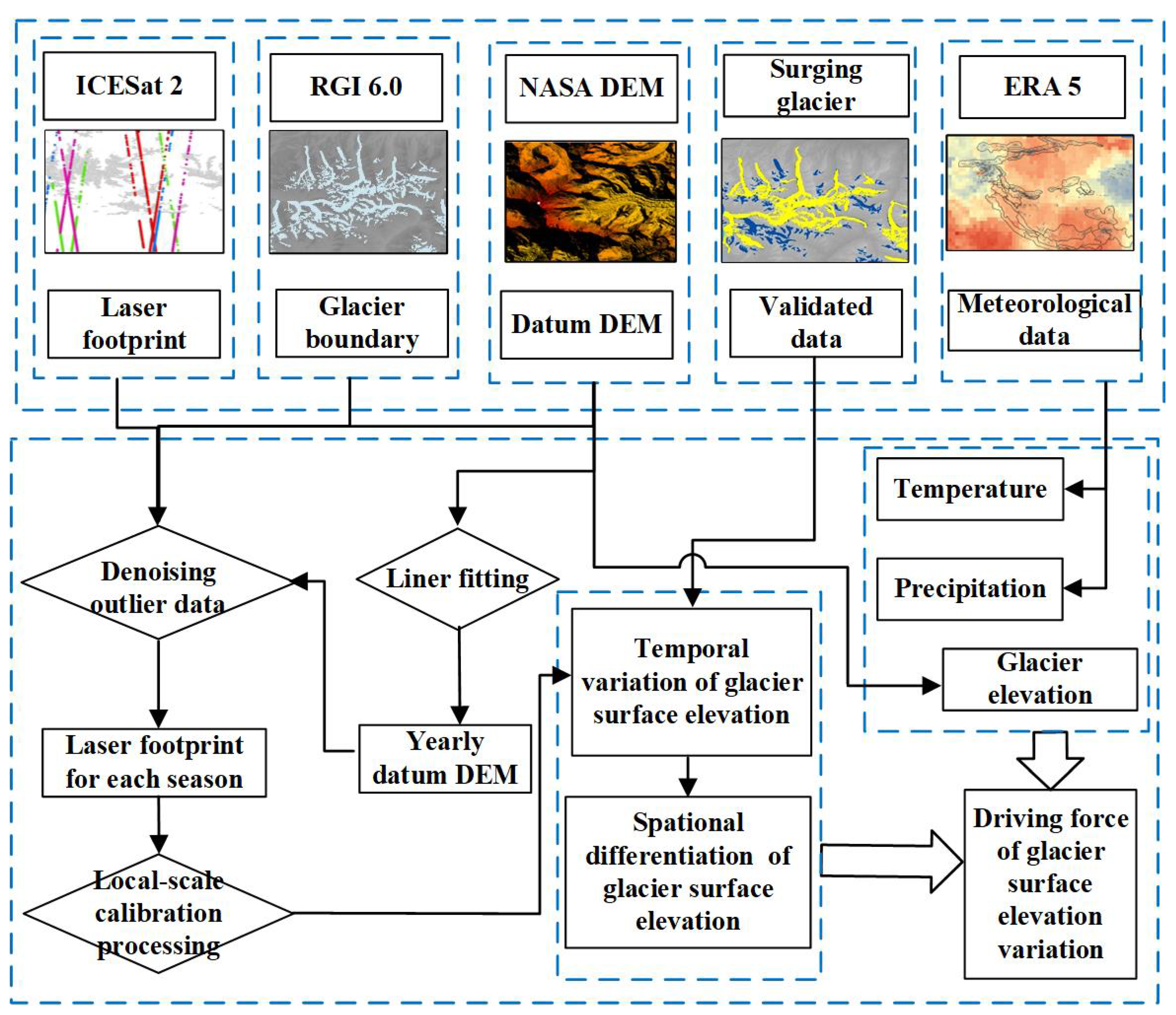
2. Data and Methodology

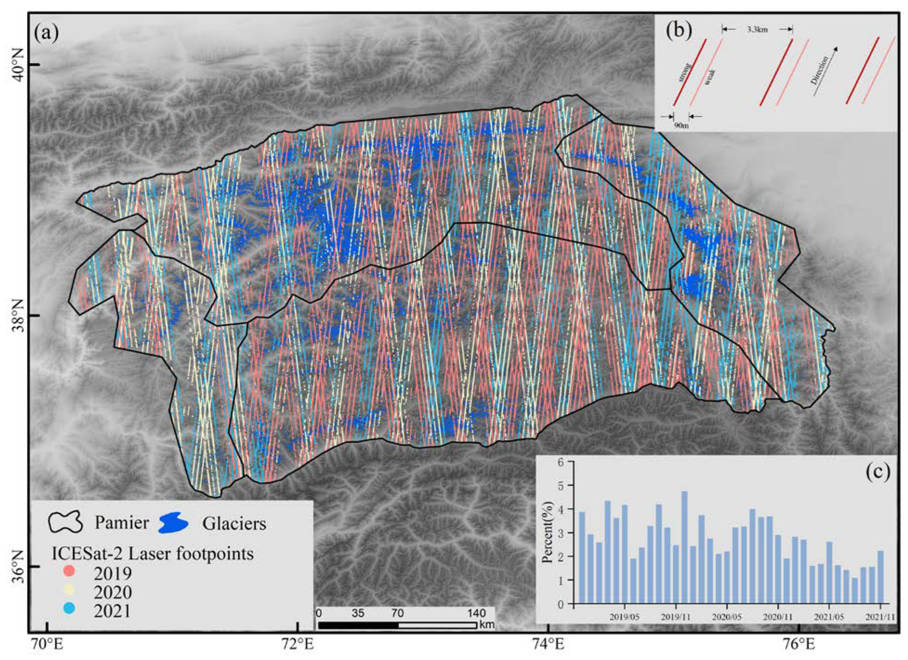
2.1. Data

To obtain surface elevation data for the glaciers in Pamir, we use the ICESat-2 level-3A land-ice height ATL06 (Advanced Topographic Laser Altimeter System 06) product for 2018–2021. The ATL06 product has better than 5 cm height accuracy and better than 20 cm surface measurement precision in the Antarctic [39,40,41,42]. The Randolph Glacier Inventory (RGI 6.0) is used to extract satellite ICESat-2 footprints within the glacier, and systematic errors are corrected using ICESat-2 data quality fields paired with glacier cataloging. Based on their research on Tibetan Plateau glaciers, Chen et al. [43] used the ICESat-2 satellite to analyze the DEM on a worldwide scale and found the NASA DEM to be the most accurate in the Central Asian alpine region. As a baseline DEM, this investigation thus uses a 30-m resolution NASA DEM that covers the study area. The NASA DEM reprocesses the raw Shuttle Radar Topography Mission (SRTM) radar signal data and telemetry data using ASTER GDEM2, ICESat, AW3D30, and other update algorithms and auxiliary data. The environmental conditions in the Pamirs are harsh, and published data from meteorological stations are scarce. The fifth generation of ECMWF atmospheric re-analyses of the global climate (ERA5) data was used to analyze the relationship between glaciers and climate in the Pamirs. ERA5 provides global month-by-month climate data with a resolution of 0.25°, including climate information such as skin_temperature and total_precipitation. Skin_temperature is a product of ERA5 data; it is the temperature of the Earth’s surface. Additionally, ERA5 has other temperature products, such as temperature_2 m, which is the temperature of air at 2 m above the surface of Earth. Total precipitation is the monthly sum of precipitation of the ERA5 data product. This article used average daily temperature and average daily precipitation calculated by skin_temperature and total precipitation to reflect climate changes.

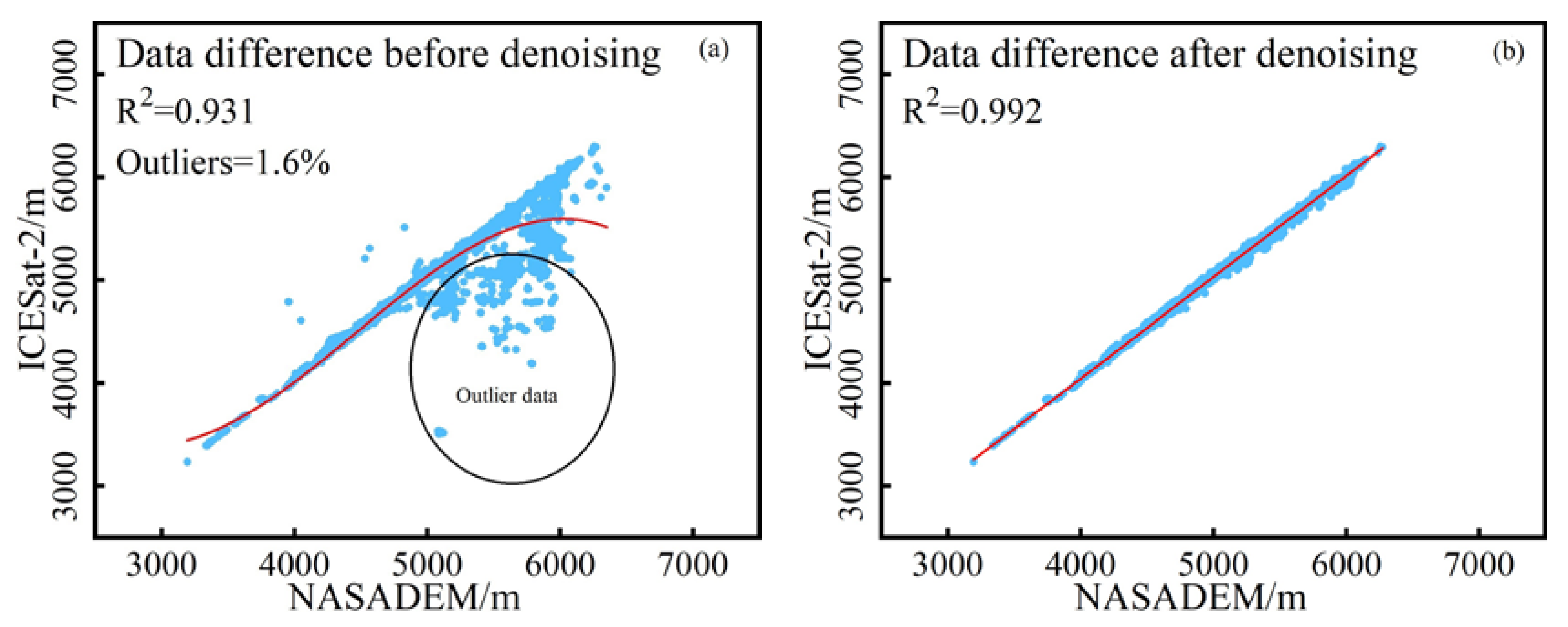
2.2. Point Cloud Denoising and Accuracy-Optimization Methods

The ATLAS laser sensor on the ICESat-2 satellite scans Earth’s surface to create two rows and three columns of reference ground tracks (Figure 2). However, the point cloud positions on a single repeat orbit do not match exactly, resulting in horizontal inaccuracies. We thus developed a point cloud denoising technique and a polynomial model to improve the spatial and temporal consistency of the ICESat-2 footprints.

Direct comparison is not possible because of the difference in ICESat-2 footprint plane positions obtained from each cycle of the point cloud data, so the NASA DEM, as a unified datum, must be used to make the ICESat-2 footprints in a small local area for different periods fall on the same plane position, and then it is important to compare the variations in elevation in that local area. We used standard deviation to reduce cloud cover and other factors from point cloud elevation anomalies, confirming the dependability of the experimental data. When the difference between all ICESat-2 footprints and the datum DEM follows a normal distribution, we let the elevation difference between the ICESat-2 footprints and the datum DEM be $D=\left[d_1,d_2,d_3,\dots ,d_{N-1},d_N\right]$, its average value be $\overline{d}$, the standard deviation be $\sigma$, the elevation of the ICESat-2 footprint be $d_i$, and N be the total number of ICESat-2 footprints. The probability that the difference between the ICESat-2 footprint and the datum DEM falls within $\left(-2\sigma ,+2\sigma \right)$ is as follows:

$$p(-2\sigma <d_i-\overline{d}<+2\sigma )\approx 95.5\%$$

(1)

An outlier is a value that deviates from the mean by more than two standard deviations (assuming that the elevation differences between the ICESat-2 footprint and the datum DEM follow a normal distribution). Although $d_i$ can be described by multiple standard deviations away from the mean in the multiple-standard-deviation approach, to confirm the correctness of the ICESat-2 footprint data, the elevations of the ICESat-2 footprint data in the study region are filtered according to the glacier inventory. We also examine the elevation differences between the ICESat-2 footprints and the datum DEM in the glacier area so that the data correspond to the normal distribution; anomalous values are excluded.

2.3. Large-Scale Variations in Yearly Time-Series Reconstruction of Glacier Surface Elevation

We use Equation (1) to eliminate the elevation of ICESat-2 footprints with low confidence and fit a polynomial model of the regional elevation to the NASA DEM elevation data as the independent variable. In this way, we determined the relationship between the yearly laser altimetry satellite point cloud elevation and NASA DEM elevation. To determine the $n\le m$ polynomial function, $Pn\left(xi\right)$, which relates $x_i$ with $y_i$, we fit points $\left(x_i,y_i\right)$ for each data set, where $i\le m$; $m$ is the number of ICESat-2 footprints; $x_i$ is the resampled NASA DEM height corresponding to the middle of ICESat-2 footprint, $i$; and $y_i$ is an elevation of the ICESat-2 footprint, $i$, in the laser point cloud. The equation for the polynomial is as follows:

$$P_n\left(x_i\right)={\displaystyle \sum }_{k=0}^n{a}_k{x}_i^k$$

(2)

where $k$ identifies the $k\mathrm{th}$ $\left(k\le n\right)$ polynomial, and $a_k$ is the polynomial coefficient obtained by fitting. The elevation produces from ICESat-2 footprint, $i$, gains in accuracy as the fitted $P_n\left(x_i\right)$ approaches $y_i$. When we obtain a minimal sum of squares, I, of the difference between the fitted elevation, $P_n\left(x_i\right)$, and the elevation, $y_i$, of all ICESat-2 footprints, the polynomial model with coefficient, $a_k$, is also more accurate. The sum of squares, I, is computed as follows:

$$I=min\left({\displaystyle \sum }_{i=0}^m{\left[P_n\left(x_i\right)-y_i\right]}^2\right)={\displaystyle \sum }_{i=0}^m{\left({\displaystyle \sum }_{k=0}^n{a}_k{x}_i^k-y_i\right)}^2$$

(3)

When the fitting function is an nth order polynomial, the $P_n\left(x_i\right)$ satisfying Equation (3) becomes the least-squares fitted polynomial. When $n=1$, it is a linear fit, and I is a multivariate function with coefficients $a_0,a_1,\dots ,a_k \left(k=0;1,\dots ,n\right)$. The above problem is equivalent to the problem of finding the extreme value $I=I\left(a_0,a_1,a_2,\dots ,a_k\right)$. For Equation (3) when $a_j$ is an unknown and the derivative of $a_j$ is equal to 0 $\left(j=0,1,\dots ,n\right)$, we obtain the necessary conditions for the multivariate function to find the extreme value:

$${\displaystyle \sum }_{i=0}^m\left({\displaystyle \sum }_{k=0}^n{a}_k{x}_i^{j+k}\right)={\displaystyle \sum }_{i=0}^n{y}_i{x}_i^j,j=0,1,\dots ,n.$$

(4)

Expanding Equation (4) about $a_j\left(j=0,1,\dots ,n\right)$ and representing the system of normal equations in matrix form leads to:

$$\left[\begin{array}{cccc}m+1& {\displaystyle {\displaystyle \sum }_{i=0}^m}{x}_i& \cdot \cdot \cdot & {\displaystyle {\displaystyle \sum }_{i=0}^m}{x}_i^n\\ {\displaystyle {\displaystyle \sum }_{i=0}^m}{x}_i& {\displaystyle {\displaystyle \sum }_{i=0}^m}{x}_i^2& \cdot \cdot \cdot & {\displaystyle {\displaystyle \sum }_{i=0}^m}{x}_i^{n+1}\\ ⋮& ⋮& ⋮& ⋮\\ {\displaystyle {\displaystyle \sum }_{i=0}^m}{x}_i^n& {\displaystyle {\displaystyle \sum }_{i=0}^m}{x}_i^{n+1}& \cdot \cdot \cdot & {\displaystyle {\displaystyle \sum }_{i=0}^m}{x}_i^{2n}\end{array}\right]\left[\begin{array}{c}{a}_0\\ a_1\\ ⋮\\ a_n\end{array}\right]=\left[\begin{array}{c}{\displaystyle {\displaystyle \sum }_{i=0}^m}{y}_i\\ {\displaystyle {\displaystyle \sum }_{i=0}^m}{x}_i{y}_i\\ ⋮\\ {\displaystyle {\displaystyle \sum }_{i=0}^m}{x}_i^n{y}_i\end{array}\right]$$

(5)

The coefficient matrix of Equation (5) is a symmetric positive definite matrix for which a unique solution exists. Based on the correlation coefficient, $R^2$, between the fitted elevation, $P_n\left(x_i\right)$, and the datum elevation, $x_i$, in the region, the nth-order polynomial is selected as the fitted polynomial to represent the fitted elevation of point cloud, $i$, and the datum DEM in the time series. The general form of the fitted polynomial is:

$$P_n\left(x_i\right)=a_n{x}_i^n+\cdot \cdot \cdot +a_2{x}_i^2+a_1{x}_i+a_0$$

(6)

where $x_i$ is the base elevation value; $P_n\left(x_i\right)$ is an elevation of the ICESat-2 footprints to be corrected; and $a_n,\dots ,a_2,a_1,a_0$ are the coefficients of the fitted polynomial. This method can establish yearly large-scale DEM information in the glacier region of the Pamir based on the NASA DEM and the yearly ICESat-2 footprints, thereby providing the production of a yearly datum DEM. This large-scale yearly DEM can be used as the datum DEM to construct the GSE in a local-scale glacier region.

2.4. Local Scale Variations in Seasonal Time-Series Reconstruction of Glacier Surface Elevation

In Section 2.3, we obtain yearly datum DEMs for large glacial regions through modeling, fitting, and interpolation. The reconstruction of the GSE in a local area requires uniform processing of the plane positions of the ICESat-2 footprints at different times (see Figure 3). Therefore, we can make the following two assumptions. (1) The elevation variation of the local area of the glacier surface is consistent in the short term. The parameter of this local area is set to 0.05 × 0.05° for this study. This size first ensures that the local area is as small as possible, and also ensures that the local area has an ICESat-2 footprint in every season, that is, every 3 months, which also provides a guarantee for the intensiveness of the time series for the local glacier area. (2) There is the elevation difference between the two ICESat-2 footprints at different times in the local glacier area after denoising. This difference is mainly caused by the terrain elevation difference in the datum DEM and the value of the GSE variation. Therefore, after unifying the plane positions of the two ICESat-2 footprints, the height difference between the two is added to the height difference caused by terrain fluctuation, which is the value of the GSE variation in this local glacier area during this period.

Figure 3 shows the main calibration processing method for calculating the plane position and elevation difference of the two ICESat-2 footprints. Figure 3a is a schematic diagram of the original two ICESat-2 footprints and the yearly datum DEM, in which the height difference of the red line is the elevation difference of the terrain fluctuation in the datum DEM of the two ICESat-2 footprints. Figure 3b is a schematic diagram of the two ICESat-2 footprints after the plane position calibration process, in which the purple line represents the value of the GSE variation during this period, and the ICESat-2 footprints obtained at the two times are located on the same plane. At this position, errors caused by terrain fluctuations are eliminated. Assuming that there are ICESat-2 footprints, after the same calibration processing, a local-scale seasonal time series reconstruction of the GSE can be achieved.

The coordinates and elevations in the ICESat-2 footprints from the glacier region are retrieved, and topographic and cloud cover anomalies are identified and removed based on the normal distribution test. Because different height-point-plane locations are generated in each cycle, point cloud data cannot be directly compared, so this local-scale calibration processing has to be used to compare the recorded variations in elevation. We use a polynomial fitting function for each season and each local area to solve the problem of incomplete matching of duplicate tracks of the ICESat-2 footprints. By performing a seasonal time series reconstruction, the polynomial fit starts with the ICESat-2 footprint elevation data from the winter of 2018 and follows the fitted heights for each season from 2018 to 2021.

Figure 4 shows the workflow of this article.

The glacier boundary in RGI 6.0 is overlayed with ICESat-2 laser footprints, and all laser footprints falling on the glacier surface from 2018 to 2021 can be obtained. Taking NASA DEM as the datum DEM, the method in Section 2.2 is used to statistically analyze the elevation difference between laser footprints and datum DEM to eliminate the laser footprints whose elevation difference exceeded 2σ; then the outliers of the laser footprints are denoised. The yearly datum DEMs are fitted by the linear relationship between the yearly laser footprints and the datum NASA DEM. Using the method shown in Section 2.3, a 0.05 × 0.05° time series of GSE variations is established. The reliability of the method in this article is verified by comparing it with the surging glacier dataset in Pamirs. The temperature and precipitation data are from the ERA5 dataset, and the relationship between climate data and GSE is analyzed by different regions and time periods.

Generally, most satellite laser footprint methods try to solve the well-posed problem of the plane positions between two footprints obtained by ICESat-1 or ICESat-2 at different times [44,45,46,47,48,49,50]. These methods are mainly based on the following assumption: that is, the acquisition times of the footprints on a single track are basically the same. The intersection of the ascending and descending tracks is adjacent to four footprints, namely the two footprints of the southeast-northwest are at time 1, and the other two footprints of the northeast and southwest are at time 2. The linear interpolation method can be used to obtain two elevation values at the two times at the intersection of the ascending and descending tracks, in other words, the variation of the GSE during this time period. Footprints of two cross-tracks can also estimate GSE variations. This cross-tracks method takes the footprints of two adjacent repeat-tracks as the processing data. The footprints of one track are projected onto the reference track. DEM is used to correct the slope difference of two adjacent repeat-tracks. The datum elevation of the footprint of another track is calculated by linear interpolation of the corresponding neighbor footprints of the reference track. The GSE variation is obtained by comparing the elevation of another track with the elevation of the footprint of the reference track after slope correction. Plane fitting of multiple adjacent repeat-tracks can also estimate the variation in GSE. This plane fitting method needs to calculate the differences between each footprint and the center footprint in the local fitting plane area, including the longitude difference, latitude difference, elevation difference, and time difference. Using these differences, an equation set of least squares plane fittings can be constructed, which can estimate the local plane eastern and northern slopes and variation in the GSE.

The method used in this article is different from other methods. The other methods mainly focus on the rate of variation of the GSE, while our method is mainly embodied in removing outliers (see Figure 5) and recalculating the elevation at a certain plane position on the glacier surface at other times. This article uses the datum DEM to calculate the datum elevation difference among two or more footprints (see the red line in Figure 3). The aim is to calibrate the plane position of the footprints in the local area. After that, multiple footprint elevations at the same plane position at different times can be obtained. The time series of the GSE can be established at this plane position. The time period of the GSE variation rate calculated by other methods mainly depends on the time of repeat-tracks or cross-tracks, and the variation rates of other time periods can be obtained by fitting the known variation rates. The time period of the method used in this article is diverse and has short time intervals. It can be used to calculate yearly or seasonal variations in the GSE. The outliers in the ICESat-1 or ICESat-2 footprints are mainly caused by the cloud and the uncertainty of the datum DEM. This article fits NASA DEM and the footprints of each year to update the yearly datum DEM. Finally, this article presents the denoising processing and plane position calibration of local footprints, which are conducive to maintaining the effective footprints and variation information of the ICESat-2 footprints as much as possible.

3. Results

3.1. Yearly Datum DEMs and Their Evaluations

Since this article uses NASA DEM as the datum for time-series reconstruction, it is necessary to match the ICESat-2 elevation with the NASA DEM. The elevation datums of NASA DEM and ICESat-2 footprints are both WGS84 reference ellipsoids. The study area is about 500 km long from east to west and about 300 km wide from north to south. Among the peak points, 160 were selected to correct the registration errors of the latitude, longitude, and elevation between the datum DEM and ICESat-2 footprints. This simple processing avoids introducing new errors due to too many control points or complex geometric correction models. A three-dimensional Google Earth with a WGS84 reference ellipsoid is used to screen and select uniformly distributed and reliable mountain top points. The latitude and longitude coordinates of 150 mountain points were recorded as the control points to register the NASA DEM and to reduce the horizontal system bias of the two sets of data. Noting the obtained glacier boundary obtained from the Randolph Glacier Inventory, the elevation points of the ICESat-2 data in the study area are selected. We use the 2019 data from Zone I (the eastern Pamir) as an example to test whether the difference between the ICESat-2 footprints and NASA DEM conformed to the normal distribution. The K-S (Kolmogorov–Smirnov) test is used to verify whether the elevation differences between the ICESat-2 footprints and the datum DEM conformed to a normal distribution. The K-S test for this elevation differences data group has a significance value of 0.3, which is greater than the significance threshold of 0.05. Therefore, it is considered that the elevation difference data follow the normal distribution. The ICESat-2 footprints with an elevation difference within two standard deviations are selected to reconstruct the time series of GSE. The ICESat-2 footprints with an elevation difference beyond one standard deviation are considered outliers (Figure 5a). These are removed to ensure the accuracy of the data. The optimized results can be seen in Figure 5b, which shows a high correlation between the elevations of ICESat-2 footprints and the elevations of the NASA DEM. At the same time, the denoised results retain the rich variation in information related to GSE at different times, and these results are differentiated from the datum DEM. In Figure 5a, before denoising, the standard deviation of the differences between ICESat-2 footprints and corresponding datum DEM was 13.9 m; in Figure 5b, after denoising, the standard deviation of the differences between ICESat-2 footprints and corresponding datum DEM was reduced to 3.6 m. The denoising process removes the outlier data (Figure 5a) and preserves the effective variational ICESat-2 footprints.

The statistical metrics coefficient of determination (R²), Root Mean Square Error (RMSE) and Outliers are used to evaluate the polynomial fit by using statistical methods to show how well the model fits the data. $R^2$ is used to express the degree of fit between the data and is given as follows:

$$R^2=\frac{SSR}{SST}=\frac{SST-SSE}{SST}=1-\frac{SSE}{SST}$$

(7)

where $SSR$ is the sum of squares of the differences between the predicted elevation and the mean of the original elevation, $SST$ is the sum of squares of the differences between the original elevation and the mean elevation, $SSE$ is the sum of squares of the errors between the points of the fit and the original data, and remains within the range [0,1]. The $SSE$ decreases and $R^2$ approaches 1 when the error decreases between the fit and the corresponding points of the original data. As a result, the closer $R^2$ is to 1, the more explanatory power the variables in the equation have for the predicted elevation, y, and the better the fit. $RMSE$ is used to measure the deviation between the ICESat-2 footprint elevation values and the yearly datum DEM. It is more sensitive to Outliers in the data, allowing for better rejection of data bias. The following is a calculation:

$$RMSE=\sqrt{\frac{1}{n}{\displaystyle \sum }_1^n{\left(H_{ICESat 2}-H_{datum DEM}\right)}^2}$$

(8)

The variable Outliers give the fraction of outliers with respect to the total data. The variation in GSE is largely affected by the glacier surface slope, elevation, accumulation, and ablation types. For the glacier physical model, a single glacier is usually divided into two regions by a certain contour line or GMB line; the upper part is the glacier accumulation area, and the lower part is the glacier ablation area. For the statistical model, there is a theoretical GMB line in the regional glacier area, which divides the glacier area into accumulation area and ablation area. The cubic polynomial can ensure good simulation of two variation trends for the accumulation and ablation zones, respectively. The quadratic has completely opposite variation trends before and after the stationary point and cannot simulate the continuous variation trends of accumulation and ablation zones. The cubic polynomial has an inflection point that can better simulate the continuous variation trends of the accumulation area and the ablation area. The quartic polynomial has two inflection points, making the variation trends of GSE too complex, which contradicts the theoretical GMB line in the statistical model. The quartic polynomial simulation will appear in multiple GMB lines, which is inconsistent with the rule of GSE variation. Thus, we assume that the relationship between the changed GSE and the datum DEM is a cubic polynomial. The elevation corresponding to the inflection point of the cubic polynomial is the elevation of the mass balance line on a large scale. The cubic polynomial fitting can ensure a good simulation of different variation trends for the accumulation and ablation zones. After many experiments, it is found that in the denoising and fitting process of the relatively sparse ICESat-1 footprints, the R² of the cubic polynomial fitting in different years can be kept above 0.98, while the R² of the linear fitting is only 0.95 at the highest. In the denoising fitting process of the relatively dense ICESat-2 footprints, the results of linear fitting and cubic polynomial fitting are similar. Additionally, R² remains above 0.99 after denoising and fitting. Here, linear fits are used to construct the yearly datum DEM.

Large-scale glacier surface elevations can be reconstructed in yearly or seasonal time series based on the NASA DEM. As shown in Figure 6, the red lines in the four subset figures are the reconstruction models for each year. The reconstructed GSE for each season from 2018 to 2021 are fit with $R^2$ > 0.99, and the ratio of the number of excluded Outliers relative to the number of seasonal data is $Outliers<1\%$. The point cloud data are fit to a polynomial to eliminate repeated orbital plane position deviations and to establish the time-series variation while conforming to the variation in GSE. ICESat-2 footprints can greatly improve the absolute accuracy of glacier elevation monitoring in alpine areas, and they can fully represent the variations in GSE in the study area.

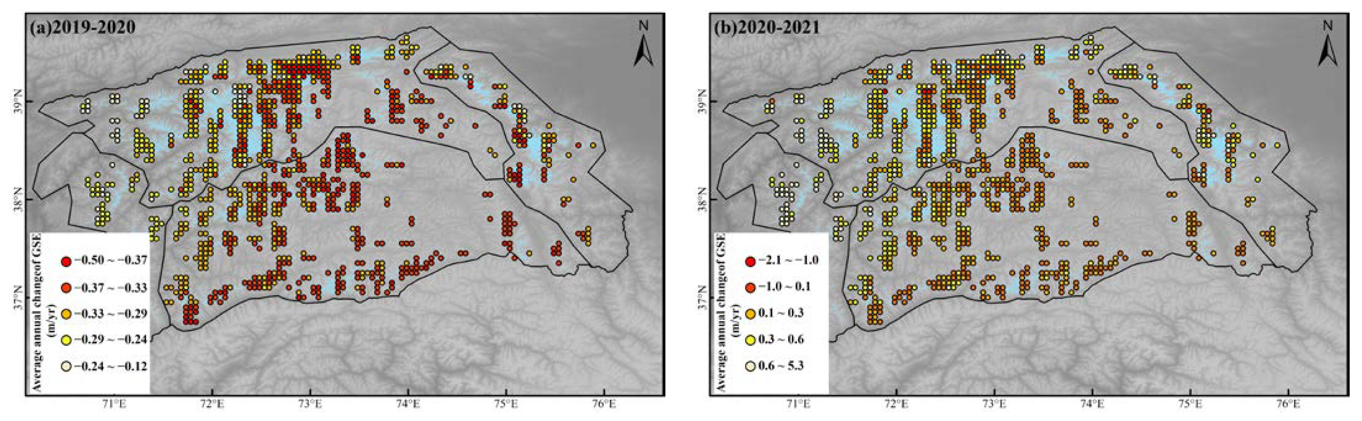
3.2. Surface Elevation Variations in Pamir Glaciers

Seasonal variations are shown in Figure 7 in four different zones from 2018 to 2021. The surface elevation of glaciers in the Pamir varies considerably in different regions due to topographic and climatic influences. The yearly DEMs modeled in Figure 6 are used as datum DEMs for seasons in one year. Using the time-series ICESat-2 footprints combined with the yearly DEMs, using the method described in Section 2.4, the seasonal time series of GSE variations are reconstructed in the scale of 0.05° × 0.05°. If the variance of the overall variation trend is greater than the mean variation value when calculating the overall or regional GSE variation trend, the trend of this time series is not obvious. Thus, it is important to remove the abnormal values and recalculate the mean and variance until the mean is greater than the variance, so that the calculated GSE variations have an obvious variation trend. Figure 7 shows the time series of seasonal variations in the GSE in the Pamir and its four subregions. From the winter of 2018 to 2021, the Pamir as a whole (meaning the glaciers in the east, south, north, and west) varies at a rate of −0.05 m/year, −0.004 m/year, −0.08 m/year, −0.04 m/year, −0.06 m/year, respectively. The seasonal variations of large-scale GSE are negative.

Glacier accumulation occurs in spring and winter, and the thickness of the accumulated snow causes fluctuations in GSE. Snowmelt occurs mainly in summer and autumn. The GSE is the highest in spring and the lowest in autumn. In this field monitoring, the snowmelt period is in April in the spring, and the freezing period is in October in the autumn. Figure 7 shows the same cycle as the practical law of glacier variations. The practical law is that glaciers accumulate in autumn and winter, while melts in spring and summer of the following year. In Figure 7, the variation trends of the GSE are similar. Figure 7 shows that the GSE increases in autumn and winter, while it decreases in spring and summer in the following year. Therefore, spring is the period of the strongest glacier accumulation, while autumn or late summer is the period of the strongest glacier ablation. For spring, the GSE was highest in 2019 and lowest in 2020. In autumn or late summer, the GSE from 2019 to 2021 was the lowest value in the year. Autumn or late summer appears to be the least affected by snow cover, and the interannual trend of GSE variation is expressed by the value in autumn or late summer.

Figure 7 shows seasonal trends in GSE; the trends of GSE in Pamir have weak downward trends in both the overall and three subregions. The seasonal monitoring results are not only related to temperature and precipitation but also to the surface topography of the Pamir glacier and the glacier movement cycle. The steep slope made it difficult for snow to remain in the glacier area. The change period of surface topography is not just one year. The factor of GSE variation affected by snow coverage is greater, which leads to inconsistency between the seasonal change in GSE and routine climate change results. We use autumn footprints of July, August, and September to calculate year-to-year changes, because the 3 months are all glacier and firn snow, least affected by new snow, and the slightly increasing trend indicates glacier surging in the future. The seasonal variations were obviously negative in Figure 7 because the steep slope and complex topography made it difficult for new snow to remain in the glacier area. It is necessary to introduce long-term monitoring results to further prove the validity of the conclusions of this article.

As shown in Figure 7 and

Table 1. Seasonal variations in GSE in Zones I–IV of the Pamir (units: m).

		Zone I	Zone II	Zone III	Zone IV	Pamir
2018 winter–2020	Winter	−0.4 ± 0.15	−0.86 ± 0.53	−0.56 ± 0.47	−0.79 ± 0.57	−0.66 ± 0.36
	Spring	−0.68 ± 0.37	−1.05 ± 0.15	−0.89 ± 0.15	−1.93 ± 0.77	−0.95 ± 0.81
	Summer	0.41 ± 0.15	−0.53 ± 0.48	0.07 ± 0.02	0.46 ± 0.17	−0.1 ± 0.04
	Autumn	0.39 ± 0.14	0.23 ± 0.18	0.21 ± 0.15	−0.22 ± 0.08	0.22 ± 0.14
	Yearly	−0.07 ± 0.05	−0.55 ± 0.12	−0.29 ± 0.18	−0.62 ± 0.19	−0.37 ± 0.12
2020–2021	Winter	0.7 ± 0.27	0.53 ± 0.5	0.56 ± 0.12	1.25 ± 0.33	0.58 ± 0.96
	Spring	0.61 ± 0.28	0.17 ± 0.09	0.35 ± 0.16	1.05 ± 0.21	0.32 ± 0.13
	Summer	0.15 ± 0.1	0.3 ± 0.12	0.16 ± 0.03	0.05 ± 0.02	0.19 ± 0.07
	Autumn	0.03 ± 0.01	−0.42 ± 0.19	−0.09 ± 0.04	−0.07 ± 0.03	−0.19 ± 0.07
	Yearly	0.36 ± 0.19	0.14 ± 0.05	0.24 ± 0.14	0.57 ± 0.13	0.23 ± 0.11

, the average elevations for each season are calculated from the regional ICESat-2 footprints. The average elevations are sorted by time, and linear regression is used to obtain the slope, amplitude, and RMSE of the regression line. In the last column, row 6 of Table 1, −0.37 is the linear regression amplitude, and ±0.12 is the RMSE. It is clear that “−0.37 m” is the varied amplitude of GSE from 2018 winter to 2020 autumn. Variation amplitudes are different among regions from winter 2018 to autumn 2020, with total yearly variation amplitudes of −0.07 ± 0.05 m, −0.55 ± 0.12 m, −0.29 ± 0.18 m, and −0.62 ± 0.19 m in Zones I–IV, respectively. The greatest reduction in GSE occurs in Zones II and IV. Winter and spring have the most significant reductions in GSE from 2018 to 2020. These seasons are periods of glacier accumulation; however, less glacier mass accumulates from winter 2019 to spring 2020 than from winter 2018 to spring 2019. The overall variation in GSE in the Pamir from 2020 to 2021 is +0.23 ± 0.11 m, with a total yearly variation of +0.36 ± 0.19 m, +0.14 ± 0.05 m, +0.24 ± 0.14 m, and +0.57 ± 0.13 m in Zones I–IV, respectively.

The consistency of the ICESat-2 footprint spatial distributions and quantities of the multi-temporal data is ensured by the method in Section 2.4. Figure 8a,b shows the spatial distributions of GSE variation trends in Pamir for 2019–2020 and 2020–2021. Each point in Figure 8 represents the variation trend obtained by linear regression of the time series of seasonal elevations. We use the slope of the linear regression formula as the variation rate and estimate regional variation trends in the GSE on a 0.05° × 0.05° geographic grid within the study area. As shown in

Table 2. Interannual variation of GSE for the Pamir.

	Average Elevation for July, August, and September 2019 (m)	Average Elevation for July, August, and September 2020 (m)	Average Elevation for July, August, and September 2021 (m)	Elevation Variation (m/Year)
Zone I	4841.177	4841.568	4841.668	+0.25 ± 0.13
Zone II	4969.066	4969.299	4968.875	−0.096 ± 0.04
Zone III	4804.549	4804.758	4804.668	+0.06 ± 0.04
Zone IV	4274.569	4274.347	4274.281	−0.14 ± 0.08
Pamir	4854.194	4854.418	4854.229	+0.02 ± 0.01

, the 2019–2020 Pamir Plateau GSE generally shows a downward trend, with a variation of −0.37 ± 0.12 m, while in 2020–2021, it shows an upward trend, with a variation of +0.23 ± 0.11. Among all zones, the GSE of Zone IV in the west has the most drastic change, with the strongest surface elevation decrease in 2019–2020 and the strongest surface elevation increase in 2020–2021. This is directly related to the lower mean value of GSE in this region, which is 4276 m, while the average glacier altitudes in the other three subregions are above 4805 m. The variation in GSE in the previous year is weak, and the surface elevation in the next year is also weak. The variation in GSE shows a strong cyclical yearly variation trend, which is a process of rising, falling, and rising for each year from 2019 to 2021.

Interannual variation is presented in Table 2. We examined variations in GSE in the research area using the Pamir autumn ICESat-2 footprints to compute the interannual rate of variation in GSE in the region. These autumn ICESat-2 footprints represent the lowest values in one year, including the ICESat-2 footprints obtained in July, August, and September. During this period of three months, the glacier surface is least disturbed by snow coverage, and these ICESat-2 footprints are a better characterization of interannual trends in GSEs. Then, the linear fit is used to obtain the variation rates in different zones. The overall GSE in the Pamir is increasing at a yearly rate of +0.02 ± 0.01 m/year, of which the variation in elevation in Zones I and III is positive (+0.25 ± 0.13 and +0.06 ± 0.04 m/year, respectively). Both Zones I and III are intensively glacierized areas, and glacier surges are frequent. The Pamir are mainly influenced by the cold weather brought about by the westerly wind belt, whereas the southeast is also influenced by the warm weather of the Indian monsoon. The surging glaciers are mainly concentrated in the eastern and northwestern parts of the Pamir. A spatial analysis of changes in glacier elevation in conjunction with the inventory of surging glaciers in the Pamir [33,51] shows that, among the approximately 13,500 glaciers in the study region, 186 have been identified as glaciers with a surging state, with 206 spatially distinct surge events identified between 1988 and 2018 [37]. There are 56 reconstructed GSE time series distributed on 44 surge glaciers, confirmed by the glacier surge inventory for the Pamir. Among them, 30 time series of GSEs covered by the data have increased, and 26 time series have decreased. These 30 time series with elevation increases are located exactly on the glacial ablation zone, and the 26 time series with elevation decreases occur on the glacial accumulation zone. The increased GSE in the ablation zone and decreased GSE in the accumulation zone further confirm the surge state of the glaciers.

Figure 9 shows that GSE is increasing mainly in the Akademiya Nauk Range and the Alay Mountains, which have large glacier concentrations and frequent glacier surges due to topography and climate change. Glaciers in Zones II and IV are mainly small valley glaciers located at relatively low altitudes and mainly on the windward slopes of the Pamir. The yearly changes in the GSE from 2018 to 2020 is −0.55 ± 0.82 and −0.62 ± 1.19 m, which is decreasing; however, the GSE has increased by 0.14 ± 0.51 and 0.57 ± 0.73 m for the years 2020 and 2021, respectively.

Zone I is the East Pamir, with 1265 glaciers and significant spatial variation in glacier variation. Overall, the surface elevation of glaciers is increasing at a rate of +0.25 ± 0.13 m/year. The areas where the GSE is increasing are mainly concentrated near Muztagh Ata–Kongur Tagh. Zone III is the most topographically complex area in the Pamir, consisting of a series of high mountain ranges and mountain valleys. It lies on the windward slopes of the westerly monsoon circulation. The westerly monsoon carries significant moisture up the valley of the Vakhsh River and its tributaries, bringing a lot of precipitation to the area. The topography and climatic conditions have densely populated the area with glaciers, making it home to the highest concentration of surge glaciers and moraine-covered glaciers. The temporal variation of the ICESat-2 footprint elevation indicates that the GSE in Zone III is increasing at a rate of +0.06 ± 0.04 m/year.

This article also uses the ICESat-2 footprints of Autumn (July, August, September) to monitor the interannual trend of GSE (Table 2). During these three months, the glacier surface is least disturbed by snow coverage. These ICESat-2 footprints are a better characterization of interannual trends in GSEs. The interannual trend of GSE derived from Autumn’s ICESat-2 footprints increased slightly because of increased precipitation and decreased temperature in Pamir. In fact, the increased precipitation can effectively ease the slope of the glacier surface; therefore, it leads to glacier accumulation in gentle slope areas or surging in the glacial terminus in Pamir.

4. Discussion

The geography of the Pamir is complicated, with tall mountains forming a massive climatic barrier to the westerly monsoon flow, resulting in high windward slopes and significant precipitation in the western region of the Pamir [52]. The climate of the Pamir is dry, with lower temperatures in the mountains caused by high altitudes, and precipitation decreasing progressively with increasing altitude in the windward zone. The winter season is dominated by cold air intrusion from the west and north, resulting in a drop in temperature and an increase in precipitation in the Pamir. The climate analysis of the Pamir used the fifth generation of ECMWF atmospheric re-analyses of the global climate (ERA5) data on mean monthly temperature and total monthly precipitation (see the results in

Table 3. Interannual variations in precipitation and temperature in the Pamir from 2018 to 2021.

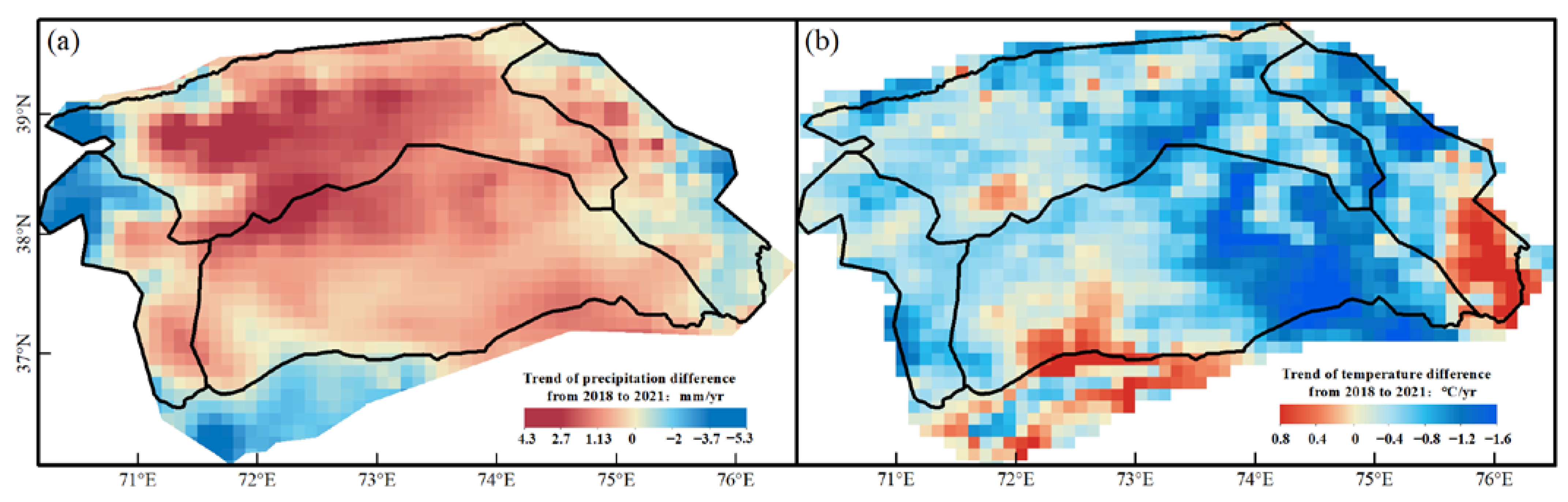
	Zone I	Zone II	Zone III	Zone IV	Pamir
Precipitation (mm/year)	−0.55 ± 0.07	+0.71 ± 0.12	+0.99 ± 0.32	−0.88 ± 0.55	+0.46 ± 0.29
Temperature (°C/year)	−0.41 ± 0.13	−0.61 ± 0.39	−0.54 ± 0.25	−0.51 ± 0.18	−0.54 ± 0.36

). The mean yearly temperature is decreasing in the study area at a rate of −0.54 ± 0.36 °C/year, and the total yearly precipitation is increasing at a rate of +0.46 ± 1.29 mm/year. The increasing GSE in the Pamir has a climatic basis, so climate change constitutes an external influence on the increasing glacial surface elevation in the region.

The average yearly temperature in the Pamir decreased by 0.54 °C from 2018 to 2021. As shown in Figure 10, this progressive decrease in temperature caused glacier melting to slow and was the climate driver for the overall increase in GSE in the Pamir [53]. In the study region, the precipitation in 2020 was 0.17 mm less than in 2019, which influenced the glacial accumulation. The GSE in all zones of the study region decreased in 2019–2020. However, precipitation in 2021 increased by 0.55 mm compared to 2020, and the GSE in the study region increased overall during this period. Climate variations and the resulting variations in GSE illustrate the complex topography of the Pamir and show that climate change is a major factor affecting GSE.

The central part of Zone II and Zone III of the Pamirs has higher elevations, and precipitation was mainly increased. The eastern part of Zone I and the western part of Zone IV are lower in elevation and mainly decreased in precipitation. From 2018 to 2021, the temperature in the Pamirs was mainly lower, with a large temperature increase in the southern part of Zone I and the southern part of Zone II, while a relatively large temperature dropped in the northeastern part of Zone I and the southeastern part of Zone II (Figure 11). It can be seen in Figure 11 that from the winter of 2018 to 2021, the overall precipitation in the Pamir increased by +0.46 ± 0.29 mm/year, while the temperature decreased by a value of −0.54 ± 0.36 °C/year. The increased precipitation and decreased temperature are both important factors causing the overall variation of GSE in this region to be +0.02 ± 0.01 m/year. In the east, when the precipitation and temperature decreased, the GSE showed an increasing trend, which was +0.25 ± 0.13 m/year, and the decreased temperature was the main reason for the increase in the GSE. In the south, when the precipitation increased and the temperature decreased, the GSE showed a decreasing trend, which was −0.096 ± 0.04, and the local temperature increase was an important reason for the slight decrease in the GSE. In the north, the precipitation increased, and the air temperature decreased, while the GSE showed a slight increasing trend (+0.06 ± 0.04 m/year). The combined effects of temperature and precipitation led to a slight increase in the surface elevation of the glacier in this area. In the west, the precipitation and temperature decreased, and the surface elevation of the glacier showed a slight decreasing trend, which was −0.14 ± 0.08 m/year. The decreased precipitation is an important reason for the decrease in the GSE. In general, the surface elevation of glaciers in the Pamir showed a slight increasing trend, and the four subregions of the GSE had different trends for temperature and precipitation, which were important factors for the differences in GSE variations.

Table 4. Comparison of research results on the different glacier variation trends in Pamir.

	Gardner et al. (2013) [7]	Gardelle et al. (2013) [9]	Kääb et al. (2015) [10]	Brun et al. (2017) [7]	This Study
Data Sources	ICESat-SRTM	ICEsat SPOT5-SRTM	ICESat	ASTER	ICESat-2 NASA DEM
Study period	2003–2009	2003–2009 2008–2011	2003–2009	2000–2016	2018–2021
GMB a	--	+0.14 ± 0.14	--	−0.08 ± 0.07	+0.017 ± 0.01
GSE b	−0.13 ± 0.22	+0.16 ± 0.15	−0.48 ± 0.14	--	+0.02 ± 0.01

^a GMB is the Glacier mass balance, in (m w.e./year); ^b GSE is the Glacier surface elevation, in (m/year).

compares the different research results of the glacier variation trends in Pamir. The variation rate of GSE monitored by ICESat-1 from 2003 to 2009 was −0.13 ± 0.22 m/year in Pamir [44]. The variation rate of GMB and GSE monitored by ICESat-1, SPOT DEM, and SRTM DEM from 2003 to 2011 was +0.14 ± 0.13 m w.e./year and +0.16 ± 0.15 m/year in Pamir [9]. The variation rate of the GMB trend in 2005–2010 at Muztag Ata in the eastern Pamirs was +0.25 m w.e./year [6]. The variation rate of GMB was −0.48 ± 0.14 m/year changing from positive to negative from 2003 to 2008 in Pamir [10]. A weak variation rate of GMB −0.08 ± 0.07 m w.e./year was found from 2000 to 2016 in Pamir [7]. These studies have all found that the Pamir glacier was in a basic equilibrium state, and the differences in the estimation results of different studies are related to factors such as data sources, glacier boundaries, estimation methods, study periods, and transformation parameters. This article uses ICESat-2 data with higher precision than ICESat-1 data. The Global Mountain Biodiversity Assessment (GMBA) Mountain Inventory was used for partitioning to study the spatial distributions of GMBs in Pamir. There were some differences in GMB in different zones, but it generally showed a weak increasing trend from winter 2018 to 2021.

5. Conclusions

Based on relatively dense satellite laser altimetry data from winter 2018 to 2021, this article analyzes variations in GSE in the Pamir. An algorithm for optimizing the denoising accuracy of point clouds in glacial areas and a long time series polynomial model for the glacier area were created using the datum DEM. The algorithms and model ensure that the point cloud data are accurate and consistent for plane positions across orbits. The results lead to the following main conclusions.

(1) Through coarse difference rejection and fitting to a polynomial, the point cloud data were related to the datum DEM elevation data. The results show that R² remains above 0.99 and that the ratio of the number of excluded Outliers relative to the number of data for each season is $Outliers<1\%$. The large-scale yearly datum DEM data for each season were fitted to a polynomial to eliminate the overall error. Repeated orbital plane errors were eliminated by the local-scale time-series reconstruction method of GSE, while allowing for computing variations in GSE. The results showed that point cloud denoising algorithms and the time-series reconstruction method improve the accuracy of surface elevation measurements for glacial areas.

(2) The trend of GSEs in the Pamir slightly increased overall at a rate of +0.02 ± 0.01 m/year. The results show that variations in GSE are strongly related to seasonal changes. Spring is the period of the strongest glacier accumulation, while autumn or late summer is the period of the strongest glacier ablation. The yearly variation of GSE shows a strong cyclical yearly variation trend, which is a process of rising, falling, and rising that was apparent from 2019 to 2021. In the western region of the Pamir, the strongest surface elevation decreased in 2019–2020, and the strongest surface elevation increased in 2020–2021. The variation of GSE in the previous year is weak, and the variation in the next year was also weak. The increase in GSE occurred mainly around Muztagh Ata–Kongur Tagh (Zone I) and Ismail Somoni Peak and Lenin Peak (Zone III). Zones I and III are all areas of massive glacial accumulation and frequent glacial surges. Time series with elevation increase was located exactly on the glacial ablation zone, and the time series with elevation decrease happened on the glacial accumulation zone. Both results demonstrate the surge state of the glacier. The results identified a surge state for 56 glaciers, which is consistent with the inventory of verified surge glaciers for the Pamir compiled by Goerlich et al. [30].

(3) Increased precipitation and decreased temperature are both important factors causing the overall variation of GSE in this region to be +0.02 ± 0.01 m/year. The GSEs in the four subregions show different variation trends due to variations in temperature and precipitation. The Pamir represents a transitional zone of climate change, so the region is subject to greater climatic influences, which leads to greater variation in glacier variation from region to region. The fifth generation of ECMWF atmospheric re-analyses of the global climate (ERA5) temperature and precipitation data was used to study climate change in the Pamir. The results indicate that the average yearly temperature change in the Pamir from 2018 to 2021 was −0.54 ± 0.36 °C/year and the total variation in precipitation was +0.46 ± 0.29 mm/year.

The results of this study reflect the complicated terrain of the Pamir and the unstable glaciers of the region. The results also show that glaciers are relatively stable despite climate change. The satellite footprint denoising accuracy optimization technique and polynomial fitting proposed herein are applicable to other altimetry data and can be used to develop an analytical model of spatial and temporal variability to better explore trends in alpine glacier regions.

References

- Sakai, A.; Fujita, K. Contrasting glacier responses to recent climate change in high-mountain Asia. Sci. Rep. 2017, 7, 13719. [Google Scholar] [CrossRef] [PubMed]
- Miles, E.; McCarthy, M.; Dehecq, A.; Kneib, M.; Fugger, S.; Pellicciotti, F. Health and sustainability of glaciers in High Mountain Asia. Nat. Commun. 2021, 12, 2868. [Google Scholar] [CrossRef]
- Bhattacharya, A.; Bolch, T.; Mukherjee, K.; King, O.; Menounos, B.; Kapitsa, V.; Neckel, N.; Yang, W.; Yao, T. High Mountain Asian glacier response to climate revealed by multi-temporal satellite observations since the 1960s. Nat. Commun. 2021, 12, 4133. [Google Scholar] [CrossRef] [PubMed]
- Francis, J.A.; Skific, N.; Vavrus, S.J. Increased persistence of large-scale circulation regimes over Asia in the era of amplified Arctic warming, past and future. Sci. Rep. 2020, 10, 14953. [Google Scholar] [CrossRef]
- Marzeion, B.; Jarosch, A.H.; Gregory, J.M. Feedbacks and mechanisms affecting the global sensitivity of glaciers to climate change. Cryosphere 2014, 8, 59–71. [Google Scholar] [CrossRef]
- Yao, T.D.; Thompson, L.; Yang, W.; Yu, W.S.; Gao, Y.; Guo, X.J.; Yang, X.X.; Duan, K.Q.; Zhao, H.B.; Xu, B.Q.; et al. Different glacier status with atmospheric circulations in Tibetan Plateau and surroundings. Nat. Clim. Chang. 2012, 2, 663–667. [Google Scholar] [CrossRef]
- Brun, F.; Berthier, E.; Wagnon, P.; Kääb, A.; Treichler, D. A spatially resolved estimate of High Mountain Asia glacier mass balances from 2000 to 2016. Nat. Geosci. 2017, 10, 668–673. [Google Scholar] [CrossRef]
- Bolch, T.; Kulkarni, A.; Kääb, A.; Huggel, C.; Paul, F.; Cogley, J.G.; Frey, H.; Kargel, J.S.; Fujita, K.; Scheel, M.; et al. The State and Fate of Himalayan Glaciers. Science 2012, 336, 310–314. [Google Scholar] [CrossRef]
- Gardelle, J.; Berthier, E.; Arnaud, Y.; Kääb, A. Region-wide glacier mass balances over the Pamir-Karakoram-Himalaya during 1999–2011. Cryosphere 2013, 7, 1263–1286. [Google Scholar] [CrossRef]
- Kääb, A.; Treichler, D.; Nuth, C.; Berthier, E. Brief Communication: Contending estimates of 2003–2008 glacier mass balance over the Pamir–Karakoram–Himalaya. Cryosphere 2015, 9, 557–564. [Google Scholar] [CrossRef]
- Farinotti, D.; Immerzeel, W.W.; De Kok, R.J.; Quincey, D.J.; Dehecq, A. Manifestations and mechanisms of the Karakoram glacier Anomaly. Nat. Geosci. 2020, 13, 8–16. [Google Scholar] [CrossRef] [PubMed]
- Treichler, D.; Kääb, A.; Salzmann, N.; Xu, C.-Y. Recent glacier and lake changes in High Mountain Asia and their relation to precipitation changes. Cryosphere 2019, 13, 2977–3005. [Google Scholar] [CrossRef]
- Berthier, E.; Brun, F. Karakoram geodetic glacier mass balances between 2008 and 2016: Persistence of the anomaly and influence of a large rock avalanche on Siachen Glacier. J. Glaciol. 2019, 65, 494–507. [Google Scholar] [CrossRef]
- Bhambri, R.; Hewitt, K.; Kawishwar, P.; Pratap, B. Surge-type and surge-modified glaciers in the Karakoram. Sci. Rep. 2017, 7, 15391. [Google Scholar] [CrossRef] [PubMed]
- Komatsu, T.; Watanabe, T. Glacier-Related Hazards and Their Assessment in the Tajik Pamir: A Short Review. Geogr. Stud. 2014, 88, 117–131. [Google Scholar] [CrossRef]
- Ren, J.; Jing, Z.; Pu, J.; Qin, X. Glacier variations and climate change in the central Himalaya over the past few decades. Ann. Glaciol. 2006, 43, 218–222. [Google Scholar] [CrossRef]
- Lüthi, M.P. Transient response of idealized glaciers to climate variations. J. Glaciol. 2009, 55, 918–930. [Google Scholar] [CrossRef][Green Version]
- Farinotti, D.; Huss, M.; Fürst, J.J.; Landmann, J.M.; Machguth, H.; Maussion, F.; Pandit, A. A consensus estimate for the ice thickness distribution of all glaciers on Earth. Nat. Geosci. 2019, 12, 168–173. [Google Scholar] [CrossRef]
- Huss, M. Density assumptions for converting geodetic glacier volume change to mass change. Cryosphere 2013, 7, 877–887. [Google Scholar] [CrossRef]
- Mayr, E.; Hagg, W. Debris-Covered Glaciers. In Geomorphology of Proglacial Systems: Landform and Sediment Dynamics in Recently Deglaciated Alpine Landscapes; Heckmann, T., Morche, D., Eds.; Springer International Publishing: Cham, Switzerland, 2019; pp. 59–71. [Google Scholar]
- Farinotti, D.; Huss, M.; Bauder, A.; Funk, M.; Truffer, M. A method to estimate the ice volume and ice-thickness distribution of alpine glaciers. J. Glaciol. 2009, 55, 422–430. [Google Scholar] [CrossRef]
- Thibert, E.; Blanc, R.; Vincent, C.; Eckert, N. Glaciological and volumetric mass-balance measurements: Error analysis over 51 years for Glacier de Sarennes, French Alps. J. Glaciol. 2008, 54, 522–532. [Google Scholar] [CrossRef]
- Uuemaa, E.; Ahi, S.; Montibeller, B.; Muru, M.; Kmoch, A. Vertical Accuracy of Freely Available Global Digital Elevation Models (ASTER, AW3D30, MERIT, TanDEM-X, SRTM, and NASADEM). Remote Sens. 2020, 12, 3482. [Google Scholar] [CrossRef]
- Zhang, Z.; Tao, P.; Liu, S.; Zhang, S.; Huang, D.; Hu, K.; Lu, Y. What controls the surging of Karayaylak glacier in eastern Pamir? New insights from remote sensing data. J. Hydrol. 2022, 607, 127577. [Google Scholar] [CrossRef]
- Du, W.; Shi, N.; Xu, L.; Zhang, S.; Ma, D.; Wang, S. Monitoring the Spatiotemporal Difference in Glacier Elevation on Bogda Mountain from 2000 to 2017. Int. J. Environ. Res. Public Health 2021, 18, 6374. [Google Scholar] [CrossRef] [PubMed]
- Du, W.; Ji, W.; Xu, L.; Wang, S. Deformation Time Series and Driving-Force Analysis of Glaciers in the Eastern Tienshan Mountains Using the SBAS InSAR Method. Int. J. Environ. Res. Public Health 2020, 17, 2836. [Google Scholar] [CrossRef] [PubMed]
- Morris, A.; Moholdt, G.; Gray, L. Spread of Svalbard Glacier Mass Loss to Barents Sea Margins Revealed by CryoSat-2. J. Geophys. Res. Earth Surf. 2020, 125, e2019JF005357. [Google Scholar] [CrossRef]
- Trantow, T.; Herzfeld, U.C.; Helm, V.; Nilsson, J. Sensitivity of glacier elevation analysis and numerical modeling to CryoSat-2 SIRAL retracking techniques. Comput. Geosci. 2021, 146, 104610. [Google Scholar] [CrossRef]
- Lin, H.; Li, G.; Cuo, L.; Hooper, A.; Ye, Q. A decreasing glacier mass balance gradient from the edge of the Upper Tarim Basin to the Karakoram during 2000–2014. Sci. Rep. 2017, 7, 6712. [Google Scholar] [CrossRef] [PubMed]
- Lv, M.; Quincey, D.J.; Guo, H.; King, O.; Liu, G.; Yan, S.; Lu, X.; Ruan, Z. Examining geodetic glacier mass balance in the eastern Pamir transition zone. J. Glaciol. 2020, 66, 927–937. [Google Scholar] [CrossRef]
- Haritashya, U.K.; Bishop, M.P.; Shroder, J.F.; Bush, A.B.G.; Bulley, H.N.N. Space-based assessment of glacier fluctuations in the Wakhan Pamir, Afghanistan. Clim. Chang. 2009, 94, 5–18. [Google Scholar] [CrossRef]
- Zhang, Z.; Xu, J.-L.; Liu, S.-Y.; Guo, W.-Q.; Wei, J.-F.; Feng, T. Glacier changes since the early 1960s, eastern Pamir, China. J. Mt. Sci. 2016, 13, 276–291. [Google Scholar] [CrossRef]
- Shangguan, D.; Liu, S.; Ding, Y.; Guo, W.; Xu, B.; Xu, J.; Jiang, Z. Characterizing the May 2015 Karayaylak Glacier surge in the eastern Pamir Plateau using remote sensing. J. Glaciol. 2016, 62, 944–953. [Google Scholar] [CrossRef]
- Snethlage, M.A.; Geschke, J.; Ranipeta, A.; Jetz, W.; Yoccoz, N.G.; Körner, C.; Spehn, E.M.; Fischer, M.; Urbach, D. A hierarchical inventory of the world’s mountains for global comparative mountain science. Sci. Data 2022, 9, 149. [Google Scholar] [CrossRef]
- Aizen, V.B.; Mayewski, P.A.; Aizen, E.M.; Joswiak, D.R.; Surazakov, A.B.; Kaspari, S.; Grigholm, B.; Krachler, M.; Handley, M.; Finaev, A. Stable-isotope and trace element time series from Fedchenko glacier (Pamirs) snow/firn cores. J. Glaciol. 2009, 55, 275–291. [Google Scholar] [CrossRef]
- Immerzeel, W.W.; Wanders, N.; Lutz, A.F.; Shea, J.M.; Bierkens, M.F.P. Reconciling high-altitude precipitation in the upper Indus basin with glacier mass balances and runoff. Hydrol. Earth Syst. Sci. 2015, 19, 4673–4687. [Google Scholar] [CrossRef]
- Goerlich, F.; Bolch, T.; Paul, F. Inventory of surging glaciers in the Pamir. Pangaea 2020. [Google Scholar] [CrossRef]
- Lv, M.; Guo, H.; Lu, X.; Liu, G.; Yan, S.; Ruan, Z.; Ding, Y.; Quincey, D.J. Characterizing the behaviour of surge- and non-surge-type glaciers in the Kingata Mountains, eastern Pamir, from 1999 to 2016. Cryosphere 2019, 13, 219–236. [Google Scholar] [CrossRef]
- Brunt, K.M.; Neumann, T.A.; Smith, B.E. Assessment of ICESat-2 Ice Sheet Surface Heights, Based on Comparisons Over the Interior of the Antarctic Ice Sheet. Geophys. Res. Lett. 2019, 46, 13072–13078. [Google Scholar] [CrossRef]
- Zhang, Y.; Pang, Y.; Cui, D.; Ma, Y.; Chen, L. Accuracy Assessment of the ICESat-2/ATL06 Product in the Qilian Mountains Based on CORS and UAV Data. IEEE J. Sel. Top. Appl. Earth Obs. Remote Sens. 2020, 14, 1558–1571. [Google Scholar] [CrossRef]
- Li, R.; Li, H.; Hao, T.; Qiao, G.; Cui, H.; He, Y.; Hai, G.; Xie, H.; Cheng, Y.; Li, B. Assessment of ICESat-2 ice surface elevations over the Chinese Antarctic Research Expedition (CHINARE) route, East Antarctica, based on coordinated multi-sensor observations. Cryosphere 2021, 15, 3083–3099. [Google Scholar] [CrossRef]
- Brunt, K.M.; Smith, B.E.; Sutterley, T.C.; Kurtz, N.T.; Neumann, T.A. Comparisons of Satellite and Airborne Altimetry with Ground-Based Data From the Interior of the Antarctic Ice Sheet. Geophys. Res. Lett. 2021, 48, e2020GL090572. [Google Scholar] [CrossRef]
- Chen, W.; Yao, T.; Zhang, G.; Li, F.; Zheng, G.; Zhou, Y.; Xu, F. Towards ice-thickness inversion: An evaluation of global digital elevation models (DEMs) in the glacierized Tibetan Plateau. Cryosphere 2022, 16, 197–218. [Google Scholar] [CrossRef]
- Gardner, A.S.; Moholdt, G.; Cogley, J.G.; Wouters, B.; Arendt, A.A.; Wahr, J.; Berthier, E.; Hock, R.; Pfeffer, W.T.; Kaser, G.; et al. A Reconciled Estimate of Glacier Contributions to Sea Level Rise: 2003 to 2009. Science 2013, 340, 852–857. [Google Scholar] [CrossRef] [PubMed]
- Moholdt, G.; Nuth, C.; Hagen, J.O.; Kohler, J. Recent elevation changes of Svalbard glaciers derived from ICESat laser altimetry. Remote Sens. Environ. 2010, 114, 2756–2767. [Google Scholar] [CrossRef]
- Wang, Q.; Yi, S.; Sun, W. Continuous Estimates of Glacier Mass Balance in High Mountain Asia Based on ICESat-1,2 and GRACE/GRACE Follow-On Data. Geophys. Res. Lett. 2021, 48, e2020GL090954. [Google Scholar] [CrossRef]
- Kääb, A.; Berthier, E.; Nuth, C.; Gardelle, J.; Arnaud, Y. Contrasting patterns of early twenty-first-century glacier mass change in the Himalayas. Nature 2012, 488, 495–498. [Google Scholar] [CrossRef]
- Hewitt, K. The Karakoram Anomaly? Glacier Expansion and the ‘Elevation Effect,’ Karakoram Himalaya. Mt. Res. Dev. 2009, 25, 332–340. [Google Scholar] [CrossRef]
- Gardelle, J.; Berthier, E.; Arnaud, Y. Slight mass gain of Karakoram glaciers in the early twenty-first century. Nat. Geosci. 2012, 5, 322–325. [Google Scholar] [CrossRef]
- Neckel, N.; Kropáček, J.; Bolch, T.; Hochschild, V. Glacier mass changes on the Tibetan Plateau 2003–2009 derived from ICESat laser altimetry measurements. Environ. Res. Lett. 2014, 9, 014009. [Google Scholar] [CrossRef]
- Kotlyakov, V.; Osipova, G.; Tsvetkov, D. Monitoring surging glaciers of the Pamirs, central Asia, from space. Ann. Glaciol. 2008, 48, 125–134. [Google Scholar] [CrossRef]
- Kapnick, S.B.; Delworth, T.L.; Ashfaq, M.; Malyshev, S.; Milly, P.C.D. Snowfall less sensitive to warming in Karakoram than in Himalayas due to a unique seasonal cycle. Nat. Geosci. 2014, 7, 834–840. [Google Scholar] [CrossRef]
- Wang, Q.; Yi, S.; Sun, W. Precipitation-driven glacier changes in the Pamir and Hindu Kush mountains. Geophys. Res. Lett. 2017, 44, 2817–2824. [Google Scholar] [CrossRef]