Article

Application of Random Forest Algorithm on Tornado Detection

1
CMA Key Laboratory of Atmospheric Sounding, Chengdu 610225, China
2
College of Electronic Engineering, Chengdu University of Information Technology, Chengdu 610225, China
3
Jiangsu Meteorological Observation Center, Nanjing 210041, China
4
State Key Laboratory of Severe Weather, Chinese Academy of Meteorological Sciences, Beijing 100081, China
*
Author to whom correspondence should be addressed.
Remote Sens. 2022, 14(19), 4909; https://doi.org/10.3390/rs14194909
Submission received: 15 August 2022 / Revised: 25 September 2022 / Accepted: 27 September 2022 / Published: 1 October 2022
(This article belongs to the Special Issue Synergetic Remote Sensing of Clouds and Precipitation)

Abstract

:
Tornadoes are highly destructive small-scale extreme weather processes in the troposphere. The weather radar is one of the most effective remote sensing devices for the monitoring and early warning of tornadoes. The existing tornado detection algorithms based on radar data are unsupervised and have strict multi-altitude constraints, such as the tornado detection algorithm based on tornado vortex signatures (TDA-TVS), which may lead to high false alarm rates, and the performance of the detection algorithm is greatly affected by the radar data quality control algorithm. A novel TDA-RF algorithm based on the random forest (RF) classification algorithm is proposed for real-time tornado identification of the S-band China new generation of Doppler weather radar (CINRAD-SA). The TDA-RF algorithm uses velocity features to identify tornadoes and adds features related to reflectivity and velocity spectrum width in radar level-II data. Historical CINRAD-SA tornado data from 2006–2015 are used to construct the tornado dataset and train the TDA-RF model. The performance of TDA-RF is evaluated using CINRAD-SA data from five tornadoes of 2016–2020 with enhanced Fujita(EF) scale ratings ranging from EF0 to EF4 and distances from 10 to 130 km to the radar. TDA-RF performs well overall with the probability of detection (POD), false alarm ratio (FAR), and critical success index (CSI) of 71%, 29%, and 55%, respectively. Moreover, the TDA-RF improves POD and CSI, and reduces FAR compared to the TDA-TVS. The maximum tornado early-warning time of TDA-RF is 17 min, and the average is 6 min; TDA-RF can provide classification probability according to the tornado generation and development process to facilitate tracking ability.

Graphical Abstract

1. Introduction

Tornadoes are small-scale cyclones generated in convective clouds and are usually closely associated with thunderstorms. The central speed of extreme event tornadoes can exceed 100 m/s, which is highly destructive, causing massive loss of life and property [1]. Tornadoes can be classified as EF0 to EF5 according to damage level and wind speed [2,3,4]. In the United States, multiple tornadoes occur in the Tornado Alley and Dixie Alley [5]. The tornado regions in the United States have a more favorable environment for supercell thunderstorms, with an average annual number of about 1200, while the annual tornado incidence in China is about 5% to 10% of that in the United States [6]. The economic losses and social impact caused by tornadoes in China are huge because tornadoes mainly occur in the densely populated and economically developed Jiangsu Province [7], although the average annual number of tornadoes in China is small. Tornadoes frequently occur in different Plains, river valleys, and coastal area provinces in the afternoon or evening during the summer months from June to August [8,9].
The Doppler weather radar is an effective device for monitoring clouds and precipitation [10]. The Doppler weather radar emits electromagnetic waves that can be scattered back to the radar by objects, such as raindrops, snowflakes, hail, bugs, and birds. The Doppler weather radar obtains weather information based on a portion of the energy returned [11]. When the weather radar observes tornadoes, different from observing raindrops (precipitation particles are relatively uniform in size), there is much debris of inconsistent sizes in tornadoes [12]. The non-uniformity of these debris makes it difficult for reflectivity to reflect tornadoes accurately. Doppler weather radars usually suffer difficulties detecting tornadoes, including speed blur, distance folding, and insufficient resolution [13,14,15]. Due to the high cost of advanced phased array radars, the use of existing operational weather radar networks to detect tornadoes has always been the focus and difficulty of meteorological researchers.
In 1975, Burgess discovered a Doppler velocity shear signature consistent with the tornado location [16], now known as the tornado vortex signature (TVS). The research on observing TVS, cyclones, and tornadoes with the Doppler weather radar [17,18], significantly promoted the development of tornado detection algorithms. In 1977, the National Severe Storms Laboratory (NSSL) analyzed multiple tornado cases and proposed the tornado vortex signature (TVS) algorithm for a tornado warning [19]. A mesocyclone is a rotating updraft within a thunderstorm, usually a supercell. Under the right conditions, a mesocyclone will tighten and intensify to produce a tornado. The mesocyclone detection algorithm (MDA) was proposed in 1985 [20], the optimization of MDA in 1998 [21], and a new tornado detection algorithm (TDA-TVS) was proposed in 1998 [22]. The TDA-TVS identifies tornado vortex signatures in radial velocity data of radar level-II data and determines whether the signatures have continuity without using reflectivity and spectral width data. As the Doppler weather radar upgraded to dual-polarization, the NSSL found the tornadic debris signature (TDS) (low cross-correlation coefficient and differential reflectivity, usually ρ H V approximately 0.8 and Z D R close to 0) and proposed the TDA-TDS algorithm in 2004 [23]. In 2015, Wang combined TDS and the Sugeno fuzzy inference system and proposed a novel tornado detection algorithm (NFTDA) [24]. The NFTDA uses differential reflectivity, cross-correlation coefficient, velocity difference, and spectrum width of the dual-polarized radar as features. With the popularity of artificial intelligence (AI) technology, complex models have been applied to the early warning and forecast of tornadoes in recent years. In 2020, Hill used several meteorological variables, including CAPE (Convective Available Potential Energy), CIN (Convective Inhibition), and wind shear, to construct a random forest prediction model for the probabilistic forecasting of severe weather in the next 1–3 days [25]. Lagerquist et al. used grided radar echo images from the fusion of multiple weather data to construct CNN networks to predict next-hour tornado occurrence [26,27]. However, the research of AI algorithms in tornado detection and prediction for CINRAD-SA is limited by radar data samples, and the research is relatively insufficient.
The S-band China new generation of Doppler weather radar (CINRAD-SA) network is the most widely deployed radar network in China [28,29]. The CINRAD-SA Doppler radar can detect the tornado parent vortex and judge the possibility of a tornado based on the characteristics of the parent vortex with algorithms such as MDA and TDA-TVS [30]. The following two problems are usually encountered when the TDA-TVS is applied to the CINRAD-SA radar. (1) The presence of noise in weather radar data, including signal processing noise and ground clutter, can significantly impact tornado identification performance; (2) The TDA-TVS algorithm determines tornado area by simultaneously finding tornado vortex signatures at multiple elevations, usually 0.5°, 1.5°, and 2.5° elevations. The effective detection distance of the TDA-TVS algorithm is about 10–100 km. The tornado vortex signature may not be detected in some elevations when the tornado occurs beyond the effective distance, which causes the TDA-TVS algorithm to fail to identify the tornado.
Machine learning can effectively reduce the impact of noise on algorithm performance and is an effective way to solve problem (1). Machine learning algorithms have specific noise adaptability [31,32] and can learn from examples, thereby reducing the impact of noise on tornado identification. For problem (2), when the vertical continuity of the tornado vortex signature cannot be satisfied, and the TDA-TVS algorithm cannot effectively identify tornadoes, applying machine learning algorithms to tornado detection is an effective way to solve this problem. However, tornadoes are low-probability and rare events in China, and the observed number of historical tornadoes is small. Deep learning methods may face the dilemma of insufficient training samples, so only machine algorithms based on small samples are available. Among the relatively mature classification techniques, such as supporting vector classifier (SVC) [33,34], logistic regression classifier (LR) [35,36], and random forest classifier (RF) [37,38], the RF has excellent advantages in nonlinearity, especially on high-dimensional datasets. In addition, tornadoes are rare events [39], and other classifiers usually overfit, while the randomness of RF can prevent overfitting [40].
This paper provides a feasible data processing method and a general framework for machine learning applications in CINRAD-SA radar for real-time tornado detection. This work uses the historical radar level-II data, reflectivity, radial velocity, and velocity spectrum to produce a tornado dataset for CINRAD-SA. A tornado detection algorithm, called TDA-RF, is constructed using the random forest algorithm. This paper is organized as follows: Section 2 presents the data format of CINRAD-SA and the process of generation of tornado samples using historical radar data. Section 3 briefly introduces the methods. Section 4 describes the model training and optimization, while Section 5 contains the experiments and results. The discussion is placed in Section 6, and the conclusions are in Section 7.

2. Data

2.1. Weather Radar Data

The CINRAD-SA radar network was gradually upgraded to dual-polarization in around 2020 in the Jiangsu Province. The tornado cases captured by the dual-polarization radar are insufficient to construct the TDA-RF model. Therefore, the historical CINRAD-SA single-polarization data was used to make the dataset. CINRAD-SA level-II data include reflectivity, radial velocity, and velocity spectrum width data. Most CINRAD-SA radars work in precipitation mode. The radar in precipitation mode scans in volume coverage pattern 21 (VCP21), and takes 6 min for each volume scan. After completing a volume scan, the level-II data is stored as radar data, containing nine elevations (0.5°, 1.5°, 2.5°, 3.4°, 4.3°, 6.0°, 10°, 14.5°, 19.5°) and 360 different radials (azimuth angle 0° to 360°). The CINRAD-SA’s resolution and detection range are shown in Table 1. For more details on CINRAD-SA radar, see Appendix A Figure A1.
The Next Generation Weather Radar (NEXRAD) is a network of 160 high-resolution S-band Doppler weather radars. The NEXRAD level-II data also contains three meteorological fundamentals: reflectivity, radial velocity, and spectrum width. Polarization data includes differential reflectivity, correlation coefficient, and differential phase. The NEXRAD has 720 radials with a distance resolution of 0.25 km between gates, and a maximum detection range is 458 km, as shown in Table 1. All the NEXRAD base data can be acquired from the NCDC website (http://www.ncdc.noaa.gov/nexradinv/, accessed on 30 September 2022).

2.2. Tornado Dataset

Level-II radar data must be preprocessed when generating tornado samples due to inconsistent distance resolution (reflectivity:1 km, radial velocity, and velocity spectrum width: 0.25 km). The 1 × 1 km reflectivity (1 point) was directly interpolated to 4 × 0.25 km (4 points) in order to keep the radar base data at the same resolution. Then, we combined the reflectivity, radial velocity, and velocity spectrum width data in the elevation and position and divided the radar data into 4 × 4 blocks. The blocks with too much invalid data and the blocks near the radar center (noisy data, about 1 to 5 km) and in the far region (distance folded or velocity ambiguity [41], usually greater than 150 km) are discarded. Each block has 4 × 4 size reflectivity, radial velocity, and velocity spectrum width, and features related to a tornado can be identified.
Tornadogenesis usually requires several conditions: shear, lift, instability, and moisture. Radar reflectivity can indicate precipitation and, to some extent, correlates with moisture conditions for tornadoes [42,43]. Therefore, the reflectivity block’s maximum, minimum, and average values are designed as features.
Weather radar radial velocity provides information about wind speed and direction, which is the component of the target’s motion along the direction of the radar beam. Positive values in radial velocity indicate wind moving from the radar, with negative values representing wind moving toward the radar. The velocity data plays an essential role in the identification of tornadoes. MDA and TDA-TVS algorithms realize early warning by detecting the radial velocity feature of the tornado vortex. In the velocity block, the features were calculated, including the radial velocity difference: Δ V (1) (to determine whether there is a positive velocity and a negative velocity, and the value of the difference), angular momentum: L (2) (calculate angular momentum between gate and gate), velocity shear: S (3) (determine the shear value of the tornado in the horizontal direction), rotational velocity: V (4) (calculate rotation speed value between gates) [44].
Δ V = V i n V o u t
L = ( V i n | + V o u t | ) × R
S = V i n | + V o u t R
V = V i n + V o u t 2
Basic velocity spectrum width measures the variability of the radial velocity estimates (movement) due to wind shear, turbulence, and the quality of the velocity samples. In the presence of tornadoes, the features presented in the velocity spectrum width are not apparent compared to the radial velocity, and the spectrum width data are seldom used. Usually, low (smooth) values of spectrum width are associated with the supercell’s rear flank downdraft, and high (chaotic) values of spectrum width are associated with tornado location. Wei [45] found that the tornado area exhibits a high spectral width value feature. Therefore, when calculating the spectral width features, the maximum, minimum, average value, the range of the spectral width block, and the thresholds were calculated in the spectral width block. Details of the above features are shown in Table A1.
After the features were calculated, all values were stored as a vector sample, the samples without Nan (NULL) value were recorded as valid data, and the location information of each block was saved. Each sample was manually labeled according to the official historical tornado records of the Jiangsu Provincial Meteorological Bureau, including time and location information. If one block was located at the tornado’s location, the vector sample corresponding to the block was marked as yes (class = 1); if the blocks did not correspond to the tornado position, the samples were labeled as no (class = 0). The flow of the tornado dataset generation is shown in Figure 1.
The dataset mainly used the lowest two-layer elevation data of radar data, including 0.5° and 1.5° elevations because most tornadoes are evident below 3 km. When the tornado exceeds 100 km from the radar, the vertical distance to the ground at elevation 2.5° and above is far more than 4 km, and weather radars are usually unable to obtain low-level information on tornadoes. This experiment mainly used the historical tornado data of Jiangsu Province from 2006 to 2021. The data from 2006 to 2015 was used to construct the tornado dataset and obtained 3590 samples, including 90 samples (class = 1) and 3500 samples (class = 0), see Table 2. There are usually 7 to 12 tornadic datapoints (class = 1) per tornado event.

3. Methods

In the subsequent sections, this paper describes how to use the random forest algorithm to construct the TDA-RF model and the testing of real tornado cases. The workflow is shown in Figure 2. The general workflow can be summarized in three parts. 1: process radar data and obtain dataset; 2: use the random forest to train the TDA-RF model, including optimization and evaluation; 3: test the optimal TDA-RF model using real tornado cases, obtain the skill scores, and compare with the TDA-TVS algorithm.

3.1. Random Forest

Random forest is a tree-based ensemble classification algorithm [37]. Random forests tend to provide a higher prediction accuracy compared to other models in classification settings [46]. A significant benefit of using random forests for classification modeling is the ability to handle datasets with a large number of predictors [47].
The random forest has sampling randomness (randomly sample the original training set to construct new training sets) and features selection randomness (randomly select a subset from all features). The randomnesses makes the algorithm usually suffer less from overfitting. About 37% of the original samples are not chosen when the samples are randomly selected. These samples are out-of-bag and can be used to evaluate and optimize the model. The random forest classifier contains multiple classification trees. When the test vector is input into the random forest classifier, each classification tree outputs the classification result, and the random forest outputs the final classification result according to the voting results of all trees and converts the voting results into probability, as shown in Figure 3.
In random forest construction and optimization, the scores of the original training set are first calculated using two criteria, Gini or Entropy. Subsequently, a subset is randomly selected from all features, and the best splitting feature is obtained using the Gini gain or Information gain algorithms, and two child nodes are obtained [48,49,50]. Finally, the above process is repeated for all child nodes until all nodes contain only one class of samples.

3.2. Features Importance

The out-of-bag samples can also evaluate the feature importance in the current dataset [51]. For a trained random forests model’s feature i, firstly, obtain the reference score ( O O B S c o r e i ) according to the out-of-bag samples:
i m p o r t a n c e i = O O B S c o r e i O O B S c o r e i r s
Secondly, randomly shuffle all the data of the out-of-bag samples under the feature i, and obtain a new score ( O O B S c o r e i r s );
Finally, calculate the difference according to Equation (5); the more significant the difference, the more critical the feature [52]. The importance of all variables can be obtained by repeating the above operations for all features. In scikit-learn, the method is ensembled as a ‘permutation feature importance’ [53].

4. TDA-RF Model Training and Optimization

When training a random forest model, it is necessary to adjust several parameters to obtain the optimal model, including the {criterion (using gini or entropy)}, {n estimators (the number of trees in the forest)}, {max features (the number of split features)}. Manually changing these parameters is usually tedious and time-consuming. The grid search algorithm is an exhaustive algorithm that obtains the optimal hyperparameters of a model over a user-specified range and interval [54].
Before model training, the dataset was randomly divided into the training set and testing set with a ratio of 0.8 and 0.2, the training samples were used to train the TDA-RF model, and the testing set was used to evaluate the TDA-RF model. In the training set, there were 72 samples (class = 1) and 2800 samples (class = 0); In the testing set, there were 18 samples (class = 1) and 700 samples (class = 0); Figure 4 shows the procedure of training and optimization.
The grid search algorithm can obtain optimal parameters over a large range after separating the training and testing sets. The parameters {criterion: entropy, n estimators: 110, max features: 5} were obtained. The grid search algorithm was used to obtain optimal parameters within a small range, and the parameters {criterion: entropy, n estimators: 102, max features: 5} (Model-1 in Figure 4) were obtained. This model was the optimal model with 32 features. After the optimal parameters, the permutation feature importance algorithm was used to obtain the features’ importance, and the results are shown in Figure 5.
In order to improve the TDA-RF model’s efficiency and reduce the negative impact of some features, the last 12 features were discarded, and the top 20 features were retained. The critical 20 features are bolded in Table A1.
In order to obtain the optimal model after optimizing the features, the TDA-RF model was retrained using the 20 features retained. The grid search algorithm was used to search the best parameters in a wide range (parameters {criterion: entropy, n estimators: 150, max features: 15} were obtained), and the optimal parameters in a small range{criterion: entropy, n estimators: 150, max features: 14} (Model-2 in Figure 4) were obtained. Under the optimal parameters, the testing set was put into the TDA-RF to obtain the evaluation scores, as shown in Section 5.1 Additionally, the TDA-RF model was tested with actual tornado cases, and the results are demonstrated in Section 5.2.

5. Experiments and Results

5.1. TDA-RF Evaluation

The testing samples were used for quantitative testing to obtain the evaluation scores for the TDA-RF model. Confusion matrices are usually used when obtaining numerical metrics for a classification model [55]. This study is a binary classification, positive samples (with a tornado in this block, class = 1) and negative samples (without tornadoes in this block, class = 0), and the binary confusion matrix is used, as shown in Table 3.
In the binary confusion matrix, T P is the number of positive samples the model outputs correctly, F P is the number of positive samples the model misclassifies, and F N is the number of negative samples the model falsely classifies. The T N is the number of negative samples that the model correctly classifies. Once the testing samples are put into the TDA-RF model, the model will output predicted labels and compare the actual labels with the predicted labels. The ACC (6), PRE (7), F1-score (8) ( R e c a l l = T P / ( T P + F N ) ), G-mean (9), POD (10), FAR (11), and CSI (12) can be obtained [56] according to the binary classification confusion matrix. These scores are shown in Table 4.
The POD-POFD and POD-SR curves are used to visualize the model’s performance, as shown in Figure 6. More details about the curves can be observed in [57].
a c c u r a c y ( A C C ) = T P + T N P C + N C
p r e c i s i o n ( P R E ) = T P T P + F P
F 1 s c o r e = 2 × R e c a l l × P r e c i s i o n R e c a l l + P r e c i s i o n
G m e a n = T P T P + F N × T N T N + F P
P O D = T P T P + F N
F A R = F P T P + F P
C S I = T P T P + F N + F P

5.2. TDA-RF versus TDA-TVS

To compare the scores of the TDA-RF and TDA-TVS algorithms, the tornado cases of 2016, 2017, 2018, and 2020 were used for testing. The time window [22] was used as the evaluation method, as shown in Figure 7. At each volume scan, if the location identified by the algorithms does not exceed 1.5 km for the center of a tornado, it is recorded as one hit; if the algorithms do not identify the tornado, it is recorded as one miss; if a tornado is incorrectly recognized, it is recorded as one false alarm. The score table after testing and statistics is shown in Table 5.

5.3. TDA-RF Tornado Detection

In order to study the performance of the TDA-RF in the operational application, use the tornado cases for evaluation. The cases met: (1) The tornado was recorded by the Jiangsu Meteorological Bureau, and the disaster investigation information includes the time, location, and intensity of the tornado. (2) The tornado occurred within 150 km from the radar center. The tornadoes identified by the TDA-RF model were marked with asterisks in the reflectivity echo map, and the values responded to the classification probability. The black circles centered on the recognition results with a radius of 1.5 km were shown in radial velocity and velocity spectrum width echo maps. The following cases were used.
The first tornado case occurred on 23 June 2016 in Funing around 14:30 (Beijing time, UTC+8). The tornado killed 99 people and injured 807. According to the data of Funing and Sheyang sounding stations (08:00, UTC+8, on 23 June 2016), the Lifted Index (LI) was −3.5 °C. The CAPE was 1408 J/kg, and the Lifting Condensation Level (LCL) was 700 m. The low-level (0–6 km) vertical wind shear reached 17 m/s. This environment was unstable, which was conducive to supercell occurrence. The tornado was an EF4, according to the disaster investigation. The Z9517 radar data was used, and the tornado was 102 km from the radar center. TDA-RF identified the tornado at 0.5° and 1.5°, as shown in Figure 8.
The second case was an EF0 tornado in Tongzhou District, Nantong, on 6 July 2016. The tornado touched the ground around 15:50 (Beijing time, UTC+8), 46 km away from the radar Z9513. The model was used to detect the tornado; the tornado was identified at 0.5° elevation at 15:52 and 15:58 (Beijing time, UTC+8), as shown in Figure 9.
The third tornado occurred in Gaoyou city on 12 June 2020. The tornado was EF3. This tornado touched down around 13:55 (Beijing time, UTC+8) and lasted for ten minutes. The Nanjing sounding data (08:00, 12 June 2020, UTC+8) demonstrated that there existed moderate-intensity CAPE (1562 J/kg), weak CIN (−6 J/kg), and strong low-level (0–3 km) wind shear (7 m/s). Such an environment was conducive to the formation and development of the convection. According to the tornado generation and development analysis [58], the initial convection of the squall line was formed at 11:00 (UTC+8). The convection continued to intensify and eventually organized into the squall line (length: 200 km, width: 25 km, and maximum reflectivity: >50 dBZ) around 12:30 (UTC+8). The rotation speed of the mesocyclone increased slowly (remaining at 10–11 m/s at the 0.5° and 1.5° elevations) before 13:30 (UTC+8). After 13:30 (UTC+8), the rotation speed began to intensify rapidly and reached the maximum around 13:48–13:54 (UTC+8). The rotation speed of the mesocyclone gradually weakened after 14:00 (UTC+8), and the squall line gradually dissipated after 14:30 (UTC+8). When the mesocyclone rotation speed reached the maximum value, the tornado occurred, so the period 13:48–14:10 (UTC+8) was used for TDA-RF testing. The 1.5° radar data of Z9250 was used for testing, and the TDA-RF detection results are shown in Figure 10 (the velocity spectrum width maps are omitted).
The fourth case is the NEXRAD radar tornado. The tornado occurred on 11 December 2021, with a damage path length of 10.5 miles, a width of 400 yards, and EF2 scale. The results are shown in Figure 11 and Figure 12. According to the NWS storm survey event report (purple tornado icon in Figure 12), the tornado occurred at 08:56 (UTC) on 1 E White Bluff, Dickson, Tennessee.

6. Discussion

In Section 4, the importance of the features was obtained using the ‘permutation feature importance’ approach. Among the 20 essential features, the c4_d_v_max, v_max, and v_min variables are related to the velocity difference, and the TDA-RF model can use these features to determine whether velocities in different directions exist and how much is the difference value in each block, which is actually consistent with crucial points of the TDA-TVS. The vt_max, c4_vt_min, c4_vt_average, c4_vt_max, vt_average features are associated with the rotational speed of a cyclone or tornado, and s_max, s_average, c4_s_min, c4_s_average are the velocity shear values for tornadoes between gates. The l_average, c4_l_average, c4_l_max, l_max are angular momentum values. The r_max, r_average variables represent that the occurrence of tornadoes usually needs a certain reflectivity value. The w_max and w_80 are spectral width features, indicating that the higher the spectrum width, the higher velocity dispersion, and the higher the probability of tornado occurrence, which is consistent with the study by Wei [45].
In Section 5.1, the scores of the TDA-RF model on the test set and the curves are obtained, where POD = 0.72, FAR = 0.13, and CSI = 0.65. Generally, for the classification model performance, AUC = 0.5 is the worst, 0.5 < AUC < 0.7 is poor, 0.7 < AUC < 0.8 is fair, 0.8 < AUC < 0.9 is good, and AUC > 0.9 is excellent [59]. From this point of view, the TDA-RF model’s performance is good (AUC = 0.84). The performance of the TDA-RF when tested on the actual tornado cases is slightly lower than the skill score on the testing set (POD: 0.71 < 0.72, FAR: 0.29 > 0.13, CSI: 0.55 < 0.65). When tested on the same cases, the TDA-RF algorithm scores are higher than the TDA-TVS algorithm (POD: 0.71 > 0.58, FAR: 0.29 < 0.39, CSI: 0.55 > 0.42), indicating that the TDA-RF outperforms the TDA-TVS.
In the first tornado case, the TDA-RF identified the tornado after it occurred. In addition to studying the effect of identification, this study examined the early warning time of TDA-RF. For example, when TDA-RF warned the first tornado case, the first warning time was at 14:15 (Beijing time, UTC+8), and the early warning time was 17 min, as shown in Appendix A Figure A2. The events in Table 5 were used for the early warning time test and yielded a maximum value of 17, a mean value of 6, and a standard deviation of 6.3.
In the second case, Δ V = V i n V o u t > 22 existed, but the radar products did not issue M or TVS warnings for this tornado. The reason is that the requirements of the M and TVS algorithms cannot be met at 1.5° elevation, as shown in Appendix A Figure A3. To a certain extent, the TDA-RF algorithm overcomes the strict limitation of traditional algorithms on multiple elevations and can play a role when the TDA-TVS algorithm fails. The TDA-RF focuses on the features of the blocks, does not compare multiple continuous elevations, and can warn more tornadoes.
In the third case, the radar Z9250 was used, which has been upgraded to dual-polarization and has reached the distance resolution of 0.25 km, so no interpolation is required when using the TDA-RF. The radar level-II data contains polarization parameters, including differential reflectivity, correlation coefficient, etc. The polarization parameters were not used when testing this case. Tornado detection results demonstrate that TDA-RF can be used for the single-polarization Doppler weather radar and dual-polarization Doppler weather radar. CINRAD-SA has only been upgraded to dual-polarization in recent years. Tornado data with polarization parameters is insufficient to construct sample sets for machine learning. Adding polarization parameters can greatly improve the identification of tornadoes [60], and the introduction of more dual-polarization features can also improve the identification effect of the TDA-RF.
In the fourth case, the NEXRAD’s KHPX radar was used. We found that the TDA-RF model was less effective at identifying tornadoes using more KHPX data. When TVS is very obvious, but the TDA-RF did not detect any tornadoes. We speculate that our model is trained based on CINRAD-SA data, and the NEXRAD’s resolution between radials is higher than CINRAD’s, which leads to the inapplicability of NEXRAD features to the TDA-RF. Therefore, the blocks with size 4x4 cannot be directly applied to the NEXRAD, and a larger block size is required.
The algorithm can provide tornado probability, which can help forecasters make better decisions. When examining the probabilities in the results, we found that the values were correlated with the tornado generation and development. The change in probability value for the third tornado case was counted and is shown in Figure 13a. For further research, the tornado that hit the city of Suqian on 22 July 2020, Jiangsu Province, at around 21:47 (Beijing time, UTC+8), was tested using the TDA-RF. The tornado lasted 3 min, and the radar Z9515 and Z9518 monitored the tornado process. The detection results are shown in Figure A4 and Figure A5. The change in statistical values is shown in Figure 13b.
In these two cases, the tornado probability demonstrated an increasing trend before the tornado occurred and gradually decreased after the tornado touched the ground. We speculate that this changing trend is related to the life cycle of tornadoes, and perhaps this trend change in tornado probability can be used to identify and warn of tornadoes. However, due to the limited tornado cases of CINRAD-SA radar and the short duration of tornadoes, it is impossible to conduct in-depth research on this trend. Subsequent research can consider applying this method to the NEXRAD radar with sufficient tornado cases while adding the relevant features of polarization parameters.
Tornadoes are rare events in China, and the class imbalance problem of samples exists in the dataset. For example, the number of the negative class is much larger than the positive class, which usually causes models to be more inclined to identify the negative class correctly. This study uses the random forests’ weight parameter {class weight} to solve this problem. Subsequent research can consider using data preprocessing and sample synthesis methods [56,61] to solve the problem and improve the model’s performance.

7. Conclusions

This paper proposes an RF-based tornado detection algorithm and applies it to CINRAD to detect tornadoes. The historical radar level-II data, including reflectivity, radial velocity, and velocity spectrum width data, are processed. The data are divided into blocks, and features are calculated. The tornado dataset is labeled according to the tornadoes’ location and time information. The tornado detection algorithm (TDA-RF) is constructed based on random forests, and the following main conclusions are obtained in the optimization and tornado case testing of the TDA-RF.
  • Features related to velocity are more critical in tornado detection; the velocity spectrum width of weather radar should be used, and features related to velocity spectrum width can improve tornado detection.
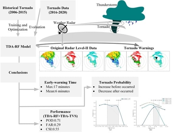
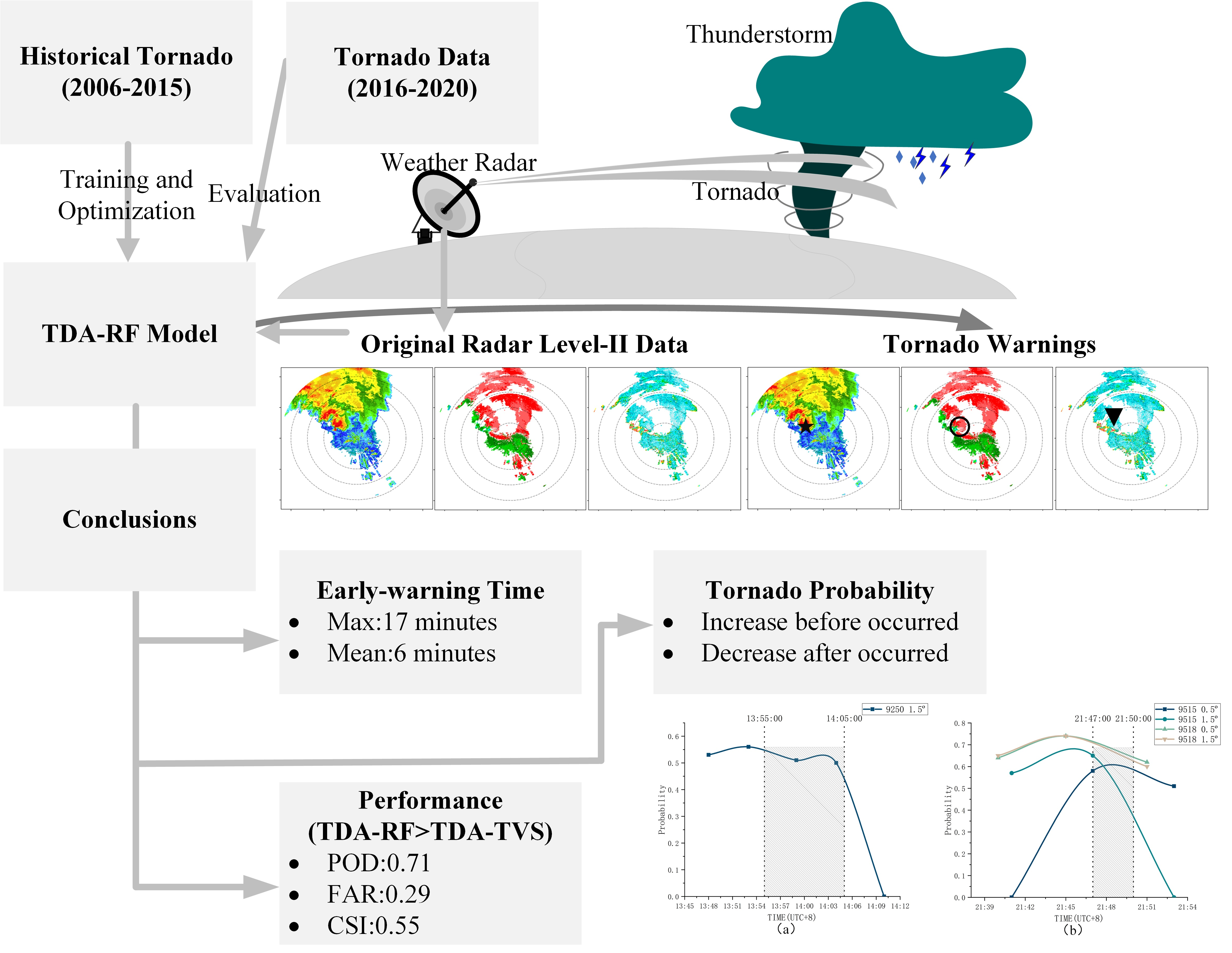
  • The maximum early-warning time of the TDA-RF for tornadoes is 17 min, and the mean value is 6 min.
  • Compared with the unsupervised tornado detection algorithm, such as the TDA-TVS, the TDA-RF uses the features in the block, classification using random forests, overcomes the limitation of multiple elevations, identifies more tornadoes, increases the probability of detection and critical success index, and reduces the false alarm rate.
  • The probability in the TDA-RF detection results is related to the tornadogenesis. The probability increases and decreases before and after the tornado touches the ground.
There are some future research directions:
  • Apply TDA-RF on NEXRAD radar data, change the block size (8 × 8 or larger), add dual polarization parameters and features, test more tornado cases, and study the change in probability;
  • Optimize the class imbalance of the tornado dataset to improve the tornado detection effect.

Author Contributions

Conceptualization, Q.Z. and Z.Q.; methodology, Q.Z.; software, Z.Q.; validation, Q.Z.; formal analysis, Q.Z.; investigation, F.Z.; resources, Q.Z. and H.W.; data curation, Q.Z.; writing—original draft preparation, Z.Q.; writing—review and editing, Q.Z., Z.Q. and H.W.; visualization, M.Z. and Q.Y.; supervision, Y.L.; project administration, Q.Z and Z.S.; funding acquisition, Q.Z. All authors have read and agreed to the published version of the manuscript.

Funding

This research was funded by the National Natural Science Foundation of China (U20B2061), the National Key R&D Program of China (2018YFC01506100), Department of Science and Technology of Sichuan Province (2020ZYD051, 2022YFS0541), the Open Grants of the State Key Laboratory of Severe Weather (2020LASW-B11), the fund of “Key Laboratory of Atmosphere Sounding, CMA” (2021KLAS01M), Key Scientific Research Projects of Jiangsu Provincial Meteorological Bureau (KZ202203) and the Key R&D Program of Yunnan Provincial Department of Science and Technology (202203AC100021).

Data Availability Statement

Not applicable.

Acknowledgments

We thank the reviewers for their constructive comments and editorial suggestions that significantly improved the quality of this paper.

Conflicts of Interest

The authors declare no conflict of interest.

Abbreviations

The following abbreviations are used in this manuscript:
TDATornado detection algorithm
RFRandom forest
TDA-RFTDA based on RF
TVSTornado vortex signature
MMesocyclone
MDAMesocyclone detection algorithm
TDA-TVSTDA based on TVS
CINRAD-SAthe S-band China new generation of Doppler weather radar
VCPVolume coverage pattern

Appendix A

Figure A1. The standard format of CINRAD-SA weather radar. The CINRAD-SA’s Nyquist velocity is 27 m/s, Pulse Repetition Frequency (PRF) 1410 Hz, and Pulse Repetition Time (PRT) 0.709 ms. The radar Level-II data were corrected, including clutter removal and velocity dealiasing.
Remotesensing 14 04909 g0a1
Table A1. The 32 features and their explanations, with the critical 20 features bolded (Z: reflectivity, V: radial velocity, W: spectrum width).
FeatureImplicationUnit
r_averageThe average value in the 4 × 4 Z blockdBZ
r_maxThe maximum value in the 4 × 4 Z blockdBZ
r_minThe minimum value in the 4 × 4 Z blockdBZ
v_averageThe average value in the 4 × 4 V blockm/s
v_maxThe maximum value in the 4 × 4 V blockm/s
v_minThe minimum value in the 4 × 4 V blockm/s
w_averageThe average value in the 4 × 4 W blockm/s
w_maxThe maximum value in the 4 × 4 W blockm/s
w_minThe minimum value in the 4 × 4 W blockm/s
s_averageThe average value of velocity shear in the 4 × 4 V block1/s
s_maxThe maximum value of velocity shear in the 4 × 4 V block1/s
s_minThe minimum value of velocity shear in the 4 × 4 V block1/s
l_averageThe average value of angular momentum in the 4 × 4 V block m 2 /s
l_maxThe maximum value of angular momentum in the 4 × 4 V block m 2 /s
l_minThe minimum value of angular momentum in the 4 × 4 V block m 2 /s
vt_averageThe average value of rotation speed in the 4 × 4 V blockm/s
vt_maxThe maximum value of rotation speed in the 4 × 4 V blockm/s
vt_minThe minimum value of rotation speed in the 4 × 4 V blockm/s
c4_d_v_maxThe maximum value of velocity difference in the 2 × 2 V blockm/s
c4_s_averageThe average value of velocity shear in the 2 × 2 V block1/s
c4_s_maxThe maximum value of velocity shear in the 2 × 2 V block1/s
c4_s_minThe minimum value of velocity shear in the 2 × 2 V block1/s
c4_l_averageThe average value of angular momentum in the 2 × 2 V block m 2 /s
c4_l_maxThe maximum value of angular momentum in the 2 × 2 V block m 2 /s
c4_l_minThe minimum value of angular momentum in the 2 × 2 V block m 2 /s
c4_vt_averageThe average value of rotation speed in the 2 × 2 V blockm/s
c4_vt_maxThe maximum value of rotation speed in the 2 × 2 V blockm/s
c4_vt_minThe minimum value of rotation speed in the 2 × 2 V blockm/s
w_rangeThe range value of velocity spectral width in the 4 × 4 W blockm/s
w_40The threshould greater than 40% velocity spectral width in the 4 × 4 W blockm/s
w_60The threshould greater than 60% velocity spectral width in the 4 × 4 W blockm/s
w_80The threshould greater than 80% velocity spectral width in the 4 × 4 W blockm/s
Figure A2. 1.5° and 0.5° Tornado early warning results (TDA-RF), Z9517-2016-0623 14:15 and 14:21 (UTC+8), the tornado was EF4. (asterisk corresponds to the identification center, and the value corresponds to the probability; the black circle has a radius of 1.5 km centered on the identification result).
Remotesensing 14 04909 g0a2
Figure A3. 1.5° radar data for the second tornado case, Z9513-2016-0706 15:52 and 15:58 (UTC+8), the tornado was EF0. The radial velocity has not any tornado vortex signaures, and TDA-TVS algorithm fails to warn the tornado.
Remotesensing 14 04909 g0a3
Figure A4. The TDA-RF detection results on radar Z9515, 0.5° and 1.5°, Z9515-2020-0722 21:41 to 21:53 (UTC+8), the tornado was EF1. (asterisk corresponds to the identification center, and the value corresponds to the probability; the black circle has a radius of 1.5km centered on the identification result; no asterisk and circle indicate that the TDA-RF did not recognize the tornado).
Remotesensing 14 04909 g0a4
Figure A5. The TDA-RF detection results on radar Z9518, 0.5° and 1.5°, Z9518-2020-0722 21:40 to 21:51 (UTC+8), the tornado was EF1. (asterisk corresponds to the identification center, and the value corresponds to the probability; the black circle has a radius of 1.5 km centered on the identification result; no asterisk and circle indicate that the TDA-RF did not recognize the tornado).
Remotesensing 14 04909 g0a5

References

  1. Nouri, N.; Devineni, N.; Were, V.; Khanbilvardi, R. Explaining the trends and variability in the United States tornado records using climate teleconnections and shifts in observational practices. Sci. Rep. 2021, 11, 1–14. [Google Scholar] [CrossRef]
  2. Ćwik, P.; McPherson, R.A.; Brooks, H.E. What is a tornado outbreak?: Perspectives through time. Bull. Am. Meteorol. Soc. 2021, 102, E817–E835. [Google Scholar] [CrossRef]
  3. McCarthy, D.; Schaefer, J.; Edwards, R. What are we doing with (or to) the F-Scale. In Proceedings of the 23rd Conference of Severe Local Storms, St. Louis, MO, USA, 5 November 2006; Volume 5. [Google Scholar]
  4. Doswell, C.A., III; Brooks, H.E.; Dotzek, N. On the implementation of the enhanced Fujita scale in the USA. Atmos. Res. 2009, 93, 554–563. [Google Scholar] [CrossRef] [Green Version]
  5. Houser, J.B.; McGinnis, N.; Butler, K.M.; Bluestein, H.B.; Snyder, J.C.; French, M.M. Statistical and empirical relationships between tornado intensity and both topography and land cover using rapid-scan radar observations and a GIS. Mon. Weather. Rev. 2020, 148, 4313–4338. [Google Scholar] [CrossRef]
  6. Zhou, R.; Meng, Z.; Bai, L. Differences in tornado activities and key tornadic environments between China and the United States. Int. J. Climatol. 2022, 42, 367–384. [Google Scholar] [CrossRef]
  7. Yu, X.; Zhao, J.; Fan, W. Tornadoes in China: Spatiotemporal distribution and environmental characteristics. J. Trop. Meteorol. 2021, 37, 681–692. [Google Scholar]
  8. Yao, Y.; Yu, X.; Zhang, Y.; Zhou, Z.; Xie, W.; Lu, Y.; Yu, J.; Wei, L. Climate analysis of tornadoes in China. J. Meteorol. Res. 2015, 29, 359–369. [Google Scholar] [CrossRef]
  9. Chen, J.; Cai, X.; Wang, H.; Kang, L.; Zhang, H.; Song, Y.; Zhu, H.; Zheng, W.; Li, F. Tornado climatology of China. Int. J. Climatol. 2018, 38, 2478–2489. [Google Scholar] [CrossRef]
  10. Kumjian, M.R. Weather radars. In Remote Sensing of Clouds and Precipitation; Springer: Berlin/Heidelberg, Germany, 2018; pp. 15–63. [Google Scholar]
  11. Doviak, R.J.; Zrnic, D.S.; Sirmans, D.S. Doppler weather radar. Proc. IEEE 1979, 67, 1522–1553. [Google Scholar] [CrossRef]
  12. Snyder, J.C.; Ryzhkov, A.V. Automated detection of polarimetric tornadic debris signatures using a hydrometeor classification algorithm. J. Appl. Meteorol. Climatol. 2015, 54, 1861–1870. [Google Scholar] [CrossRef]
  13. Chu, Z.; Yin, Y.; Gu, S. Characteristics of velocity ambiguity for CINRAD-SA Doppler weather radars. Asia-Pac. J. Atmos. Sci. 2014, 50, 221–227. [Google Scholar] [CrossRef]
  14. Frank, L.R.; Galinsky, V.L.; Orf, L.; Wurman, J. Dynamic multiscale modes of severe storm structure detected in mobile Doppler radar data by entropy field decomposition. J. Atmos. Sci. 2018, 75, 709–730. [Google Scholar] [CrossRef]
  15. Zhang, X.; He, J.; Zeng, Q.; Shi, Z. Weather radar echo super-resolution reconstruction based on nonlocal self-similarity sparse representation. Atmosphere 2019, 10, 254. [Google Scholar] [CrossRef] [Green Version]
  16. Burgess, D.W.; Lemon, L.R.; Brown, R.A. Tornado characteristics revealed by Doppler radar. Geophys. Res. Lett. 1975, 2, 183–184. [Google Scholar] [CrossRef]
  17. Wakimoto, R.M.; Wilson, J.W. Non-supercell tornadoes. Mon. Weather. Rev. 1989, 117, 1113–1140. [Google Scholar] [CrossRef]
  18. Lemon, L.R.; Donaldson, R.J., Jr.; Burgess, D.W.; Brown, R.A. Doppler radar application to severe thunderstorm study and potential real-time warning. Bull. Am. Meteorol. Soc. 1977, 58, 1187–1193. [Google Scholar] [CrossRef]
  19. Brown, R.A.; Lemon, L.R.; Burgess, D.W. Tornado detection by pulsed Doppler radar. Mon. Weather. Rev. 1978, 106, 29–38. [Google Scholar] [CrossRef]
  20. Zrnić, D.; Burgess, D.; Hennington, L. Automatic detection of mesocyclonic shear with Doppler radar. J. Atmos. Ocean. Technol. 1985, 2, 425–438. [Google Scholar] [CrossRef]
  21. Stumpf, G.J.; Witt, A.; Mitchell, E.D.; Spencer, P.L.; Johnson, J.; Eilts, M.D.; Thomas, K.W.; Burgess, D.W. The National Severe Storms Laboratory mesocyclone detection algorithm for the WSR-88D. Weather. Forecast. 1998, 13, 304–326. [Google Scholar] [CrossRef]
  22. Mitchell, E.D.W.; Vasiloff, S.V.; Stumpf, G.J.; Witt, A.; Eilts, M.D.; Johnson, J.; Thomas, K.W. The National Severe Storms Laboratory tornado detection algorithm. Weather. Forecast. 1998, 13, 352–366. [Google Scholar] [CrossRef]
  23. Ryzhkov, A.V.; Schuur, T.J.; Burgess, D.W.; Zrnic, D.S. Polarimetric tornado detection. J. Appl. Meteorol. 2005, 44, 557–570. [Google Scholar] [CrossRef]
  24. Wang, Y.; Yu, T.Y. Novel tornado detection using an adaptive neuro-fuzzy system with S-band polarimetric weather radar. J. Atmos. Ocean. Technol. 2015, 32, 195–208. [Google Scholar] [CrossRef]
  25. Hill, A.J.; Herman, G.R.; Schumacher, R.S. Forecasting severe weather with random forests. Mon. Weather. Rev. 2020, 148, 2135–2161. [Google Scholar] [CrossRef] [Green Version]
  26. Basalyga, J.N.; Barajas, C.A.; Gobbert, M.K.; Wang, J.W. Performance benchmarking of parallel hyperparameter tuning for deep learning based tornado predictions. Big Data Res. 2021, 25, 100212. [Google Scholar] [CrossRef]
  27. Lagerquist, R.; McGovern, A.; Homeyer, C.R.; Gagne, D.J., II; Smith, T. Deep learning on three-dimensional multiscale data for next-hour tornado prediction. Mon. Weather. Rev. 2020, 148, 2837–2861. [Google Scholar] [CrossRef]
  28. Min, C.; Chen, S.; Gourley, J.J.; Chen, H.; Zhang, A.; Huang, Y.; Huang, C. Coverage of China new generation weather radar network. Adv. Meteorol. 2019, 2019, 5789358. [Google Scholar] [CrossRef]
  29. Jianxin, H. CINRAD WSR-98D and its ground clutter filter design. In Proceedings of the 2001 CIE International Conference on Radar Proceedings (Cat No. 01TH8559), Beijing, China, 15–18 October 2001; pp. 1186–1189. [Google Scholar]
  30. Wang, B.; Wei, M.; Hua, W.; Zhang, Y.; Wen, X.; Zheng, J.; Li, N.; Li, H.; Wu, Y.; Zhu, J. Characteristics and possible formation mechanisms of severe storms in the outer rainbands of Typhoon Mujiga (1522). J. Meteorol. Res. 2017, 31, 612–624. [Google Scholar] [CrossRef]
  31. Zhang, W.; Peng, G.; Li, C.; Chen, Y.; Zhang, Z. A new deep learning model for fault diagnosis with good anti-noise and domain adaptation ability on raw vibration signals. Sensors 2017, 17, 425. [Google Scholar] [CrossRef] [Green Version]
  32. Li, Z.; Meier, M.A.; Hauksson, E.; Zhan, Z.; Andrews, J. Machine learning seismic wave discrimination: Application to earthquake early warning. Geophys. Res. Lett. 2018, 45, 4773–4779. [Google Scholar] [CrossRef] [Green Version]
  33. Cortes, C.; Vapnik, V. Support-vector networks. Mach. Learn. 1995, 20, 273–297. [Google Scholar] [CrossRef]
  34. Chang, C.C.; Lin, C.J. LIBSVM: A library for support vector machines. ACM Trans. Intell. Syst. Technol. 2011, 2, 1–27. [Google Scholar] [CrossRef]
  35. Wright, R.E. Logistic regression. In Reading and Understanding Multivariate Statistics; American Psychological Association: Washington, DC, USA, 1995; pp. 217–244. [Google Scholar]
  36. Tsangaratos, P.; Ilia, I. Comparison of a logistic regression and Naïve Bayes classifier in landslide susceptibility assessments: The influence of models complexity and training dataset size. Catena 2016, 145, 164–179. [Google Scholar] [CrossRef]
  37. Breiman, L. Random forests. Mach. Learn. 2001, 45, 5–32. [Google Scholar] [CrossRef] [Green Version]
  38. Pal, M. Random forest classifier for remote sensing classification. Int. J. Remote Sens. 2005, 26, 217–222. [Google Scholar] [CrossRef]
  39. Maalouf, M.; Homouz, D.; Trafalis, T.B. Logistic regression in large rare events and imbalanced data: A performance comparison of prior correction and weighting methods. Comput. Intell. 2018, 34, 161–174. [Google Scholar] [CrossRef]
  40. Peerbhay, K.Y.; Mutanga, O.; Ismail, R. Random forests unsupervised classification: The detection and mapping of solanum mauritianum infestations in plantation forestry using hyperspectral data. IEEE J. Sel. Top. Appl. Earth Obs. Remote Sens. 2015, 8, 3107–3122. [Google Scholar] [CrossRef]
  41. Schvartzman, D.; Curtis, C.D. Signal processing and radar characteristics (SPARC) simulator: A flexible dual-polarization weather-radar signal simulation framework based on preexisting radar-variable data. IEEE J. Sel. Top. Appl. Earth Obs. Remote Sens. 2018, 12, 135–150. [Google Scholar] [CrossRef]
  42. Austin, P.M. Relation between measured radar reflectivity and surface rainfall. Mon. Weather. Rev. 1987, 115, 1053–1070. [Google Scholar] [CrossRef]
  43. Honda, T.; Amemiya, A.; Otsuka, S.; Taylor, J.; Maejima, Y.; Nishizawa, S.; Yamaura, T.; Sueki, K.; Tomita, H.; Miyoshi, T. Advantage of 30-s-updating numerical weather prediction with a phased-array weather radar over operational nowcast for a convective precipitation system. Geophys. Res. Lett. 2022, 49, 1–9. [Google Scholar] [CrossRef]
  44. Hengstebeck, T.; Wapler, K.; Heizenreder, D.; Joe, P. Radar network-based detection of mesocyclones at the German weather service. J. Atmos. Ocean. Technol. 2018, 35, 299–321. [Google Scholar] [CrossRef]
  45. Wang, B.; Wei, M.; Fan, G.; Du, A. The evolution and mechanism of tornadic supercells in the outer rainbands of strong typhoon Mujigae (1522). Part I: Spectrum width and mesocyclone speed. J. Trop. Meteorol. 2018, 34, 472–480. [Google Scholar]
  46. Fernández-Delgado, M.; Cernadas, E.; Barro, S.; Amorim, D. Do we need hundreds of classifiers to solve real world classification problems? J. Mach. Learn. Res. 2014, 15, 3133–3181. [Google Scholar]
  47. Speiser, J.L.; Miller, M.E.; Tooze, J.; Ip, E. A comparison of random forest variable selection methods for classification prediction modeling. Expert Syst. Appl. 2019, 134, 93–101. [Google Scholar] [CrossRef]
  48. Quinlan, J.R. C4. 5: Programs for Machine Learning; Elsevier: Amsterdam, The Netherlands, 2014. [Google Scholar]
  49. Loh, W.Y. Classification and regression trees. Wiley Interdiscip. Rev. Data Min. Knowl. Discov. 2011, 1, 14–23. [Google Scholar] [CrossRef]
  50. Raileanu, L.E.; Stoffel, K. Theoretical comparison between the gini index and information gain criteria. Ann. Math. Artif. Intell. 2004, 41, 77–93. [Google Scholar] [CrossRef]
  51. Genuer, R.; Poggi, J.M.; Tuleau-Malot, C. Variable selection using random forests. Pattern Recognit. Lett. 2010, 31, 2225–2236. [Google Scholar] [CrossRef] [Green Version]
  52. Huang, N.; Lu, G.; Xu, D. A permutation importance-based feature selection method for short-term electricity load forecasting using random forest. Energies 2016, 9, 767. [Google Scholar] [CrossRef] [Green Version]
  53. Pedregosa, F.; Varoquaux, G.; Gramfort, A.; Michel, V.; Thirion, B.; Grisel, O.; Blondel, M.; Prettenhofer, P.; Weiss, R.; Dubourg, V.; et al. Scikit-learn: Machine learning in python. J. Mach. Learn. Res. 2011, 12, 2825–2830. [Google Scholar]
  54. Ramadhan, M.M.; Sitanggang, I.S.; Nasution, F.R.; Ghifari, A. Parameter tuning in random forest based on grid search method for gender classification based on voice frequency. DEStech Trans. Comput. Sci. Eng. 2017, 10. [Google Scholar] [CrossRef] [Green Version]
  55. Luque, A.; Carrasco, A.; Martín, A.; de Las Heras, A. The impact of class imbalance in classification performance metrics based on the binary confusion matrix. Pattern Recognit. 2019, 91, 216–231. [Google Scholar] [CrossRef]
  56. He, H.B.; Garcia, E.A. Learning from imbalanced data. IEEE Trans. Knowl. Data Eng. 2009, 21, 1263–1284. [Google Scholar] [CrossRef]
  57. Lagerquist, R.; Gagne, D., II. Basic Machine Learning for Predicting Thunderstorm Rotation: Python Tutorial; 2019. [Google Scholar]
  58. Tang, J.; Tang, X.; Xu, F.; Zhang, F. Multi-scale interaction between a squall line and a supercell and its impact on the genesis of the “0612” Gaoyou tornado. Atmosphere 2022, 13, 272. [Google Scholar] [CrossRef]
  59. Adams, M.A.; Johnson, W.D.; Tudor-Locke, C. Steps/day translation of the moderate-to-vigorous physical activity guideline for children and adolescents. Int. J. Behav. Nutr. Phys. Act. 2013, 10, 49. [Google Scholar] [CrossRef] [Green Version]
  60. Lim, S.; Allabakash, S.; Jang, B.; Chandrasekar, V. Polarimetric radar signatures of a rare tornado event over south Korea. J. Atmos. Ocean. Technol. 2018, 35, 1977–1997. [Google Scholar] [CrossRef]
  61. Qing, Z.; Zeng, Q.; Wang, H.; Liu, Y.; Xiong, T.; Zhang, S. ADASYN-LOF algorithm for imbalanced tornado samples. Atmosphere 2022, 13, 544. [Google Scholar] [CrossRef]
Figure 1. The generation flow of tornado dataset. (Firstly, divide the radar into many blocks; then, calculate the tornado-related features in each block; finally, label the samples according to tornado time and position information, and obtain the tornado dataset).
Remotesensing 14 04909 g001
Figure 2. The workflow of this paper. The part 1 corresponds to Section 2, part 2 represents Section 3 and Section 4, and part 3 indicates Section 5.
Remotesensing 14 04909 g002
Figure 3. The random forest classifier. The random forest outputs the final class and probabilities based on the voting results.
Remotesensing 14 04909 g003
Figure 4. The flow of the TDA-RF model training and optimization. (The ‘parameters’ obtained from the GridSearch were used as input for the next GridSearch or to obtain the optimal model; Model-1 was the optimal model with 32 features, and Model-2 was optimal with 20 features).
Remotesensing 14 04909 g004
Figure 5. The score of features’ importance, top 20 essential features score greater than 2.77.
Remotesensing 14 04909 g005
Figure 6. The POD-POFD and POD-SR curves on the testing set. The Area Under the Curve (AUC) is 0.84, and the maximum Critical Success Index (CSI) is 0.65.
Remotesensing 14 04909 g006
Figure 7. The time window used for scoring the TDA-RF and TDA-TVS. The beginning ( T b e g i n ) and ending ( T e n d ) times of a tornado event are also indicated.
Remotesensing 14 04909 g007
Figure 8. 0.5° and 1.5° tornado detection results (TDA-RF), Z9517-20160623-14:32 (UTC+8), the tornado was EF4. (asterisk corresponds to the identification center, and the value corresponds to the probability; the black circle has a radius of 1.5 km centered on the identification result).
Remotesensing 14 04909 g008
Figure 9. 0.5° tornado detection results (TDA-RF), Z9513-20160706-15:52 and 15:58 (UTC+8), the tornado was EF0. (asterisk corresponds to the identification center, and the value corresponds to the probability; the black circle has a radius of 1.5 km centered on the identification result).
Remotesensing 14 04909 g009
Figure 10. 1.5° tornado detection results (TDA-RF), Z9250-0612-13:48 to 14:10 (UTC+8), the tornado was EF3. (asterisk corresponds to the identification center, and the value corresponds to the probability; the black circle has a radius of 1.5 km centered on the identification result; no asterisk and circle indicate that the TDA-RF did not recognize the tornado).
Remotesensing 14 04909 g010
Figure 11. TDA-RF detection results on NEXRAD radar data. KHPX radar 2021-12-11 08:55 (UTC), the tornado was EF2. (The inverted triangle is the warning result of GR2Analyst, and the asterisk and circle are the warning result of TDA-RF).
Remotesensing 14 04909 g011
Figure 12. TDA-RF detection results on NEXRAD radar data. KHPX radar 2021-12-11 08:58 (UTC), the tornado was EF2. (The inverted triangle is the warning result of GR2Analyst, the asterisk and circle are the warning result of TDA-RF).
Remotesensing 14 04909 g012
Figure 13. The change of probability in the results of the third tornado case with time. (a): Tornado case on 12 June 2020. (b): Tornado case on 22 July 2020. (When TDA-RF does not recognize a tornado, the probability is set to 0. The shaded area is the tornado duration).
Remotesensing 14 04909 g013
Table 1. The level-II data information for CINRAD and NEXRAD. The reflectivity, radial velocity, and spectrum width are three meteorological fundamentals for weather radars. The polarization data are not listed.
RadarInformationReflectivityRadial VelocitySpectrum Width
CINRAD-SADistance resolution1 km0.25 km0.25 km
Maximum detection range460 km230 km230 km
Format for each data9 × 360 × 4609 × 360 × 9209 × 360 × 920
NEXRADDistance resolution0.25 km0.25 km0.25 km
Maximum detection range458 km458 km458 km
Format for each data9270 × 18329270 × 18329270 × 1832
Table 2. Historical tornado events from 2006–2015 were used to build the tornado dataset and train the TDA-RF model. The position represents latitude and longitude, respectively.
Date (UTC+8)PositionIntensityRadar
20060703 20:01–20:13119.781,33.551EF1Z9515,Z9516
20070703 16:40–17:20119.229,32.650EF3Z9250
20080817 15:05–15:15120.355,33.581EF2Z9515
20090827 15:30–16:15120.980,31.385EF0Z9513
20100717 19:30–19:35116.563,34.677EF1Z9516
20110822 06:00–06:10120.042,31.873EF0Z9519
20130707 16:40–17:15119.645,32.833EF0Z9517,Z9523
20140824 15:40–15:50119.656,32.629EF2Z9523
20150724 12:15–12:18119.436,32.776EF0Z9523
Table 3. Binary confusion matrix.
True Class
model predict class positive (yes tornado)negative (no tornado)
Y (yes tornado) T P (True Positives) F P (False Positives)
N (no tornado) F N (False Negatives) T N (True Negatives)
column counts P C = T P + F N N C = F P + T N
Table 4. The TDA-RF scores on the testing set.
ACCPREF1-ScoreG-MeanPODFARCSI
0.99030.86670.78780.84860.72220.13330.65
Table 5. TDA-RF and TDA-TVS scores. The position represents latitude and longitude, respectively. H: numbers of hits, M: numbers of misses, F: numbers of false alarms (F). POD = H/(H + M), FAR = F/(H + F), and CSI = H/(H + M + F).
TDA-RFTDA-TVS
RadarDate(UTC+8)PositionIntensityHMFHMF
Z9515,Z951720160623
14:15–14:30
119.803,33.694EF4411322
Z9517,Z951920160706
15:50–16:00
121.012,31.940EF0412321
Z9515,Z952320170702
11:00–11:15
120.483,32.673EF1421424
Z952720180818
18:40–19:05
117.052,34.339EF2322232
Z925020200612
13:55–14:10
119.451,32.741EF3211210
Total 177714109
Score POD:0.71
FAR:0.29
CSI:0.55
POD:0.58
FAR:0.39
CSI:0.42
Publisher’s Note: MDPI stays neutral with regard to jurisdictional claims in published maps and institutional affiliations.

