Communication

Spatiotemporal Prediction of Monthly Sea Subsurface Temperature Fields Using a 3D U-Net-Based Model

1
The College of Meteorology and Oceanography, National University of Defense Technology, Changsha 410005, China
2
Independent Researcher, Mailbox No. 5111, Beijing 100094, China
*
Author to whom correspondence should be addressed.
Remote Sens. 2022, 14(19), 4890; https://doi.org/10.3390/rs14194890
Submission received: 25 August 2022 / Revised: 26 September 2022 / Accepted: 27 September 2022 / Published: 30 September 2022
(This article belongs to the Special Issue AI for Marine, Ocean and Climate Change Monitoring)

Abstract

:
The ability to monitor and predict sea temperature is crucial for determining the likelihood that ocean-related events will occur. However, most studies have focused on predicting sea surface temperature, and less attention has been paid to predicting sea subsurface temperature (SSbT), which can reflect the thermal state of the entire ocean. In this study, we use a 3D U-Net model to predict the SSbT in the upper 400 m of the Pacific Ocean and its adjacent oceans for lead times of 12 months. Two reconstructed SSbT products are added to the training set to solve the problem of insufficient observation data. Experimental results indicate that this method can predict the ocean temperature more accurately than previous methods in most depth layers. The root mean square error and mean absolute error of the predicted SSbT fields for all lead times are within 0.5–0.7 °C and 0.3–0.45 °C, respectively, while the average correlation coefficient scores of the predicted SSbT profiles are above 0.96 for almost all lead times. In addition, a case study qualitatively demonstrates that the 3D U-Net model can predict realistic SSbT variations in the study area and, thus, facilitate understanding of future changes in the thermal state of the subsurface ocean.

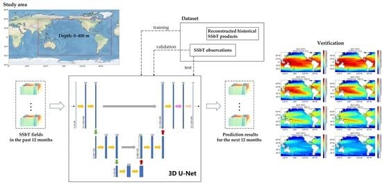
Graphical Abstract

1. Introduction

In oceanographic investigations, the sea temperature is a crucial measure that can indicate the thermal state of seawater [1]. Its variation strongly correlates with the global climate and meteorological events [2,3,4,5] and can affect the marine ecological environment, underwater acoustic communication, and commercial fisheries [6,7,8]. Therefore, sea temperature prediction is crucial for assisting in the early assessment of the likelihood of associated events. Two categories can be used to group the methods for predicting sea temperature. The first group is based on dynamical models to simulate atmosphere–ocean variables with physical constraints and then make forecasts [9,10,11]. The second group attempts to capture the relationships between past observations and future sea temperature through data analysis. This group includes statistical model-based approaches [12,13] and machine learning-based approaches [14,15,16,17]. In the last two decades, machine learning-based approaches have been increasingly adopted to predict sea temperature due to lower computational costs and higher flexibility in comparison with numerical model-based approaches [18,19]. For example, to estimate the time series of sea surface temperature (SST) in isolated locations, Zhang et al. [17] used long short-term memory (LSTM). The gated recurrent unit model, which has less trainable parameters compared with LSTM, was used by Zhang et al. [20] for SST time series prediction. Yang et al. [21] used a fully connected LSTM (FC-LSTM) layer and a convolution layer to predict the SST of an area of nearby points to incorporate the temporal and spatial information. However, the abovementioned models cannot capture the spatial linkage of the sea temperature values in a large region, thus limiting their prediction performance. Researchers have paid close attention to the performance of the convolutional LSTM (ConvLSTM) model in precipitation nowcasting [22]. This model replaces the matrix operations of the FC-LSTM with convolutions, making it a powerful tool that can extract expressive spatial feature maps of input images and model their time evolution. The ConvLSTM model has been used in some studies to successfully estimate sea temperature [23,24,25].
Sea subsurface temperature (SSbT), which is a 3D sea temperature field, is essential for understanding the mechanisms and processes in the ocean as a whole [26] and is thus preferred in oceanographic studies [27]. A review of previous studies revealed that the prediction of the SSbT has not been investigated as extensively as that of the SST. Liu et al. [28] employed LSTM to predict the mean seawater temperature at various depths at each observation point for the following month. To predict the SSbT for 3-day and 5-day lead times at an observation point, Patil and Iiyama [29] first used a ConvLSTM network to extract the spatiotemporal information of the past SST around this point and then used a multilayer perceptron to analyze the past observed SSbT profiles at this point. The results of the prediction were then produced by combining the outputs of these two networks. Zhang et al. [25] used a multilayer ConvLSTM (M-ConvLSTM) model to predict the mean SSbT field of the upcoming month in a subarea of the Pacific Ocean in terms of the spatiotemporal prediction of the SSbT in a region rather than at specific points. To solve the extraction problem of 3D spatial correlation of the SSbT field, a 4D convolutional neural network (CNN) was designed by Zuo et al. [30] for SSbT horizontal and profile prediction of the next day, respectively, in which a 4D convolution operation was implemented by linearly adding the results of several 3D convolution operations. Although deep learning (DL) has significantly improved SSbT prediction, there are still few studies that perform SSbT field prediction for lead times greater than 1 month, which limits their usefulness as a reference for longer-term ocean-related studies. Moreover, an insufficient amount of monthly observation data limits the generalization ability of the network during training.
This study investigates the DL-based long-term SSbT field prediction. Utilizing the SSbT fields from the previous 12 months as the input, a 3D U-Net-based model was constructed to perform the prediction of the monthly SSbT fields, mostly in the Pacific Ocean, for lead times up to 12 months. This model is capable of extracting the spatiotemporal features of historical SSbT fields and mapping them into future SSbT fields. In addition, two SSbT products that have been recreated based on objective analysis have been added to the training dataset to address the issue of insufficient monthly mean observation data. The rest of this manuscript is organized as follows. Section 2 briefly introduces some related works about SSbT prediction. Section 3 describes the data used in this study. The suggested approach is illustrated in Section 4. Section 5 presents the experimental findings. Finally, Section 6 provides the conclusions of this study.

2. Related Works

Liu et al. [28] considers the spatiotemporal SSbT field prediction as a combination of the independent time series prediction of each observation point in a 3D grid region. They first use a matrix fusion approach to capture the features of the closeness and period in the temperature time series and then leverage LSTM to conduct the temperature prediction for the next month. This method is evaluated at different depth levels of three regions, including the Coral Sea, the equatorial Pacific Ocean, and the South China Sea. Experimental results show that the optimal parameters of the fusion matrix are different for different depth levels. Comparable or even better overall performance is achieved by using this method compared to support vector regression and a multilayer perceptron. However, the spatiotemporal relationship between observation points is ignored in the modeling process, which limits the prediction performance.
Instead of using a DL model to predict the temperature of each depth layer separately, Patil and Iiyama [29] investigate the DL-based SSbT profile prediction for 3-day and 5-day lead times at a specific location in the eastern Indian Ocean. In their developed model, a ConvLSTM network is first adopted to extract the spatiotemporal features of the past SST around this location. Then, a multilayer perceptron is used to extract the patterns of the past observed SSbT profiles at this location. Finally, these two types of features are fused by another multilayer perceptron to generate the prediction result. Experimental results show that compared with using SST only, the prediction accuracy can be significantly improved by incorporating the past SSbT profiles into the model. In addition, it is found that the proposed model produces higher prediction errors for the intermediate depth levels from 100 m to 300 m compared to other depth levels.
To model the spatiotemporal relationship of the sea temperature in the whole 3D grid region, Zhang et al. [25] and Zuo et al. [30] propose the M-ConvLSTM model and 4D-CNN model, respectively. Zhang et al. [25] focus on predicting the mean SSbT field of the next month based on monthly mean SSbT fields of the previous 28 months. The input SSbT field at each time step is considered as a multi-channel image. The M-ConvLSTM model, which consists of multiple ConvLSTM layers, is used to transmit and update the inner states along the time direction of the input sequence of SSbT fields. The prediction result is generated at the last time step. The M-ConvLSTM model achieves improvements over the FC-LSTM model [21] for SST prediction. The coefficient of determination for most depth layers exceeds 0.95. Zuo et al. [30] develop a 4D-CNN-based model to perform SSbT horizontal and profile prediction of the next day, respectively. The 4-D convolution module is the core part of this model. When conducting SSbT horizontal prediction, they first divide the SSbT fields into several temporal sequences of horizontal fields according to depth levels. Then, different 3D convolutional layers are applied to the temporal sequences of different depths, and their outputs are added up to enrich feature representation. As for the SSbT profile prediction, the SSbT fields are divided into several temporal sequences of profiles along the latitude, and then the 4-D convolution module is used to extract their features. Experiments show that this model achieves competitive performance when predicting the sea temperature for different depth levels, locations and seasonal thermocline. This method requires a lot of parameters and computation when there are many depth levels for SSbT horizontal prediction or many latitudes for SSbT profile prediction.

3. Data

The study area, which includes the Pacific Ocean, the eastern Indian Ocean, and the western Atlantic Ocean, is located between latitudes 59.5°S and 59.5°N and longitudes 95.5°E and 25.5°W, as shown in Figure 1.
The SSbT data used in this investigation are monthly mean sea temperature in the upper 400 m over the study area. The depth levels are 0, 10, 20, 30, 50, 75, 100, 150, 200, 250, 300, and 400 m. The amount of data available for neural network training is insufficient since accurate SSbT observations with full spatial and temporal coverage are only available after the early 1980s. Therefore, the reconstructed historical SSbT products provided by the Institute of Atmospheric Physics (IAP) [27] and the Research Data Archive (RDA) at the National Center for Atmospheric Research [31] are added to the training set to increase the sample size and avoid the overfitting problem in the training process. As for SSbT observations, the SST data are from the National Oceanic and Atmospheric Administration (NOAA) Optimum Interpolation SST V2 (OISST V2) dataset [32], and data of seawater temperature at depths of 10 to 400 m are from the Global Ocean Data Assimilation System (GODAS) at the National Centers for Environmental Prediction (NCEP) [33]. To make the GODAS data consistent with the reconstructed products, bilinear interpolation (a widely accepted and often used interpolation algorithm that can resample the grid products to a new resolution [34,35]) was utilized to adjust the horizontal spatial (latitude–longitude) resolution from 0.333° × 1° to 1° × 1°. In addition, if one product does not have the data for one selected depth level, the sea temperature fields at close levels would be linearly interpolated to this level. After the data processing was complete, spatiotemporal sequences were produced for each type of monthly SSbT product using a 24-month sliding window with a sliding step of 1 month.
Regarding the division of these generated sequences, all reconstructed SSbT sequences and most of the observation sequences were used for training, and the remaining observation sequences were used for validation and testing. In addition, we prevented time overlap between the target SSbT fields in the training, validation, and test set sequences. For details, see Table 1.

4. Method

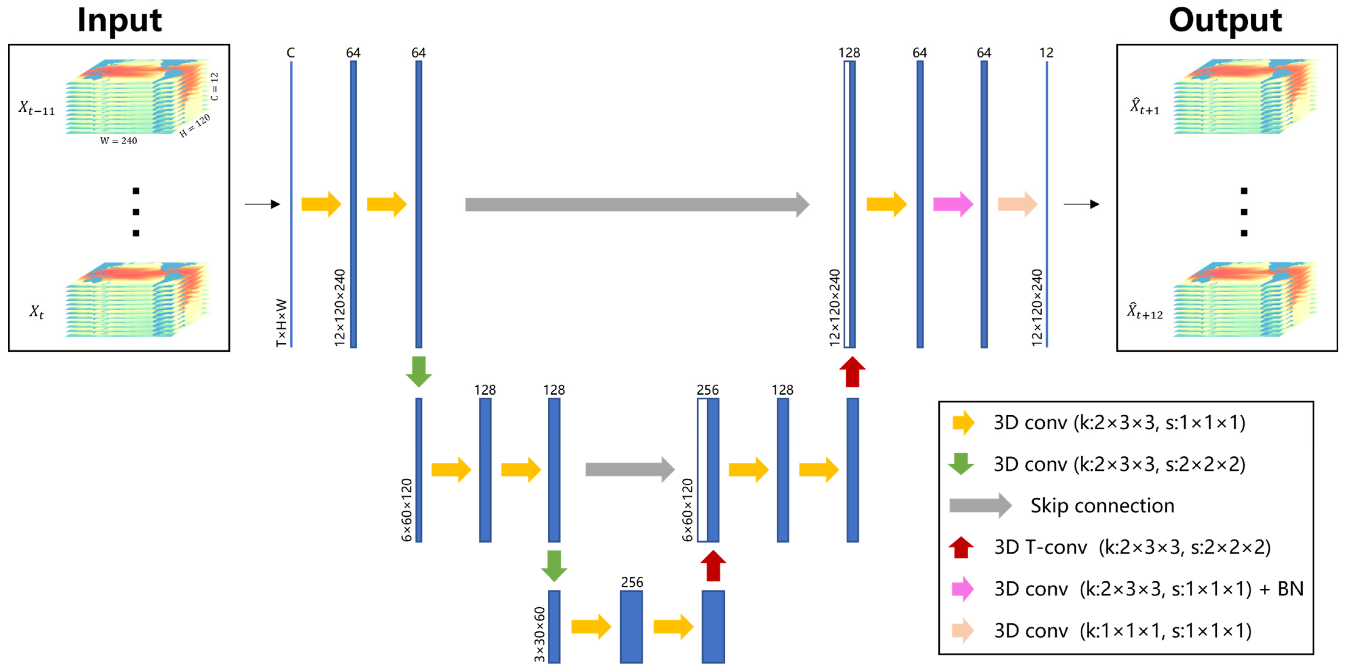
When modeling, the shape of the input data or feature map tensors is (T, H, W, C). Here, T, H, W, and C refer to the time, height, width, and channel dimensions, respectively. Specifically, for the input sequence of SSbT fields for the previous 12 months, T is 12 (number of timesteps), H is 120 (latitude grid size), W is 240 (longitude grid size), and C is 12 (number of depth levels).
The created model, which is shown in Figure 2, is an end-to-end trainable model-based on the 3D U-Net model [36], which was designed initially for volumetric segmentation. It is composed of multiple 3D convolutional layers, each of which is followed by a rectified linear unit activation function, except for the final convolutional layer. This model, like U-Net, has a downsampling path, a symmetrical upsampling path, and skip connections.
In the downsampling path, the temporal and spatial sizes of the input sequence are progressively halved by using two 3D convolutional layers with strides of 2, each of which is followed by two 3D convolutional layers, and spatiotemporal features with different representation levels are extracted. Two transposed 3D convolutional layers, each of which is followed by two more 3D convolutional layers, are used in the upsampling process to gradually restore the high-level features to their original size. Furthermore, low-level features are received from the downsampling path through skip connections, delivering detailed information to generate more comprehensive representations. To speed up model training, batch normalization (BN) [37] is performed after the second-to-last convolutional layer. The predicted monthly SSbT fields are output through the final convolutional layer with a kernel size of 1 × 1 × 1.
The root mean square error (RMSE) is utilized as the loss function to guide the training of the developed model in this study, which is defined as
L R M S E = m = 1 12 1 N n = 1 N ( X ^ t + m ( n ) X t + m ( n ) ) 2
where X ^ t + m ( n ) is the value of the n grid point of the predicted SSbT field for the time step t + m , and X t + m ( n ) is the corresponding ground truth value.

5. Experiments

5.1. Experimental Settings

A seasonal naïve model that copies the input SSbT fields from the past 12 months unaltered to its outputs (assuming the interannual variation of SSbT is zero), M-ConvLSTM model [25], and a simple 3D-CNN (S3D-CNN) [38] are three baselines against which the 3D U-Net model is compared. The temperature values are normalized by dividing by 30 before being input into the models. All the DL-based models are trained using the RMSE loss function defined in Section 4 for a fair comparison. The learning rate is set at 0.0001, and the batch size is 4. When the validation loss does not decrease for 12 epochs, the training process is terminated to prevent overfitting. The training plots of the 3D U-Net model are shown in Figure 3. These DL-based models are implemented using TensorFlow [39] and run on a TITAN RTX GPU (24 GB).

5.2. Evaluation Metrics

RMSE and mean absolute error (MAE) are used to measure the SSbT prediction error, which is defined as
R M S E = 1 N n = 1 N ( X ^ ( n ) X ( n ) ) 2
M A E = 1 N n = 1 N X ^ ( n ) X ( n )
A correlation coefficient (CC) is adopted to evaluate the consistency between the observed SSbT profile s and the predicted SSbT profile s ^ at the i , j observation point, which is defined as
C C i , j = C o v ( s ^ , s ) V a r ( s ^ ) V a r ( s )
The average CC of all observation points of the predicted SSbT field can be calculated as
C C = 1 H W i = 1 H j = 1 W C C i , j

5.3. Results

We compared the prediction performance of the model between training on observation-only data and training on observation and reconstruction data. The results are shown in Table 2, in which 12-month average RMSE, MAE, and CC are adopted as indicators. Using additional reconstruction data resulted in relative improvements of 7.5% and 9.3% in terms of RMSE and MAE, while the CC value increased from 0.9506 to 0.9616. This proves that the reconstructed historical data can help improve the overall performance of the model for SSbT prediction.
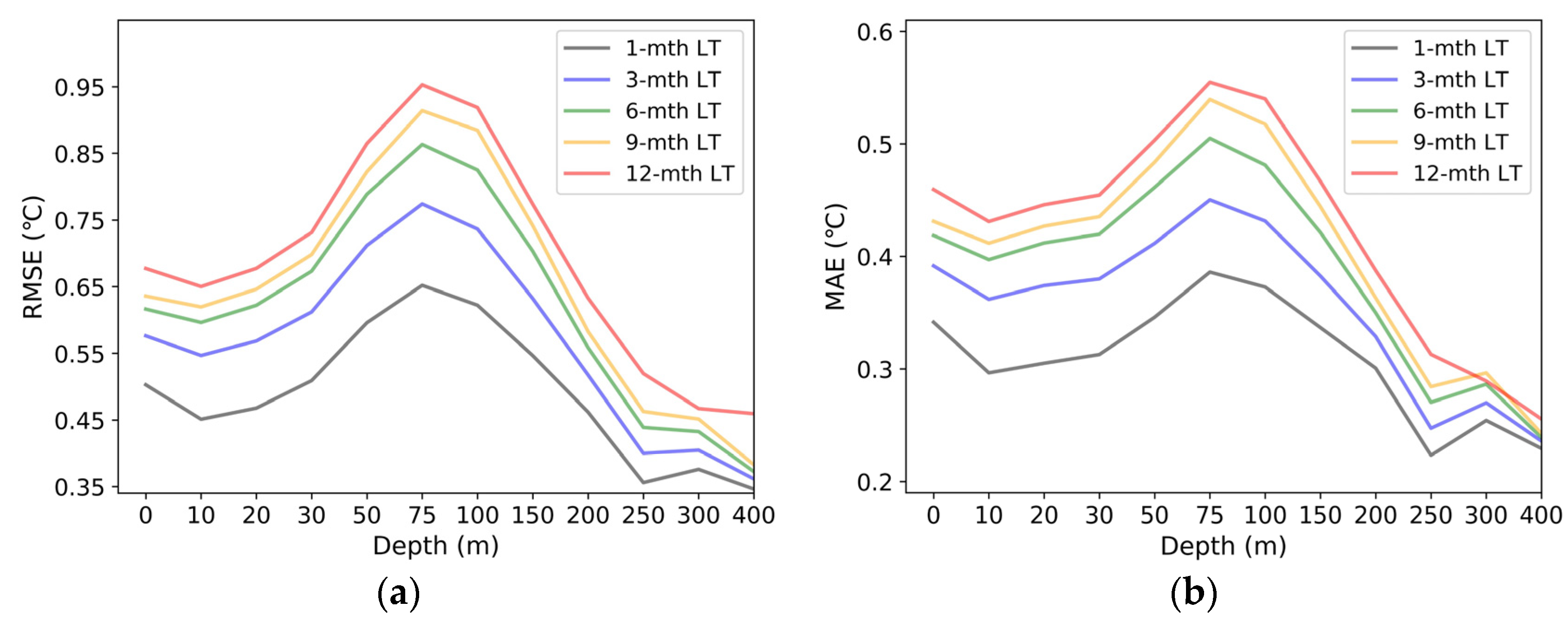
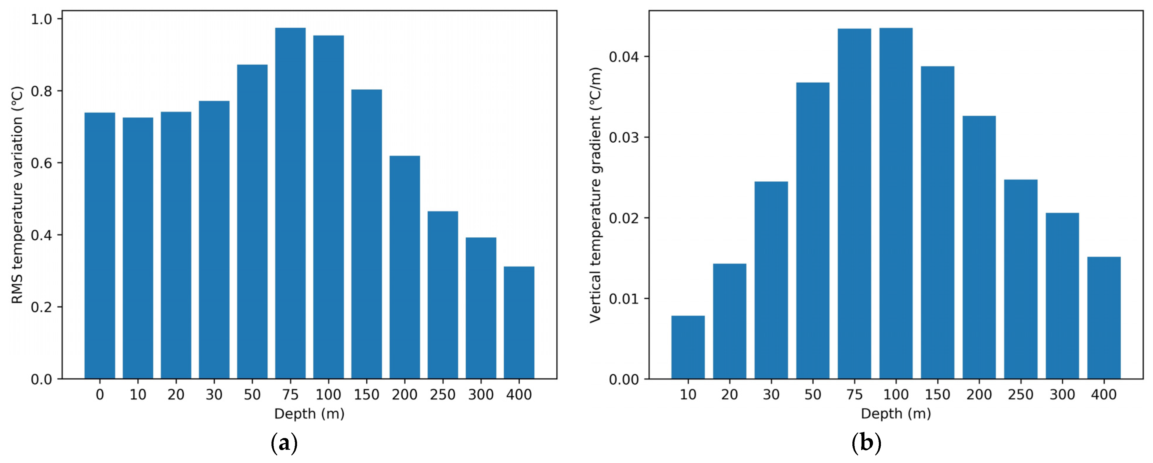
The verification of depth levels for lead times of 1, 3, 6, 9, and 12 months is shown in Figure 4. For all depth levels, the 3D U-Net model’s temperature prediction error increased with growing lead times. The prediction performance of the model varied at different depths. In general, the prediction error of SST and 50–150 m SSbT is larger than that at other depths. Relatively large prediction error obtained at 0 m may be due to the presence of more erratic elements, such as solar radiation and sea surface winds. To investigate the reasons for the large prediction error at the depth of 50–150 m, we calculated the average root-mean-square (RMS) values of the temperature inter-annual variations for different depth levels, as shown in Figure 5a. It can be seen that the subsurface temperature inter-annual variability peaks in the range 50–150 m, which is consistent with the findings in [40], making it difficult to accurately model the temporal variations at these depth levels. In addition, the vertical temperature gradients for different depth levels was computed. As shown in Figure 5b, the vertical temperature gradients are higher at the depth of 50–150 m than those at other depth levels, which also causes a significant prediction error.
We then examined the prediction performance of this method for SSbT in different geographical parts of the study area, including north temperate (between 35.5°N–59.5°N), north subtropics (between 23.5°N–35.5°N), tropics (between 23.5°N–23.5°S), south subtropics (between 23.5°S–35.5°S), and south temperate (between 35.5°S–59.5°S). First, the prediction performance for different depth levels over these regions were examined. For simplicity and intuition, six depth levels at appropriate intervals were selected within 0–400 m, including 0, 20, 50, 100, 200, and 400 m. The 12-month average RMSE values are shown in Table 3. The SST prediction error in tropics is lower than in other regions. However, the highest RMSE values are obtained for the prediction of temperature at depths of 50, 100, and 200 m over this region. The changes in prediction error with depth in north temperate, north subtropics and tropics are generally consistent with the trend of the whole study area (shown in Figure 4), while the prediction error in south subtropics and south temperate increases with depth. Beyond that, the overall prediction performance for all 12 depth levels in the upper 400 m over the six regions was evaluated using 12-month average RMSE, MAE, and CC as indicators. As shown in Table 4, the RMSE and MAE values are higher in tropics than in other regions, in which the error produced in middle layers contributes a lot. It seems that the prediction performance for SSbT in the Southern Hemisphere is better than that in the Northern Hemisphere, and the prediction error in subtropical zones is lower than that in temperate zones. It is noteworthy that the CC values of the predicted SSbT profiles in subtropical and tropical zones are above 0.99, while those of north temperate and south temperate are around 0.91. This indicates that the predicted SSbT profiles in temperate zones has poorer consistency with the observations compared to that in other regions.
For lead times of 1–12 months, the SSbT prediction performance of different methods was examined at depths of 0, 20, 50, 100, 200, and 400 m. As shown in Figure 6, the prediction error of the seasonal naïve model for a specific depth is positively correlated with the inter-annual variation of temperature at that depth. Three DL models outperformed the seasonal naïve model for most of the selected depths. However, they are worse than the seasonal naïve model for 400 m where the inter-annual variation of temperature at 400 m is much smaller compared to those at other depth levels. This is probably because redundant layers in these DL models cause a loss of input information. The use of residual blocks [41] may alleviate this problem. In comparison to the M-ConvLSTM model, it was found that the S3D-CNN and 3D U-Net models had reduced RMSE values for all the chosen depth levels at all lead times, demonstrating their potential in modeling spatiotemporal data with seasonal periodicity. In addition, the designed 3D U-Net model is superior to the M-ConvLSTM and S3D-CNN models for these depth levels.
For all 12 depth levels, the total prediction performance of the comparative approaches was assessed. The results are displayed in Figure 7. It can be seen that the 3D U-Net model has a lower prediction error than the other methods for all lead times. The CC values obtained by the four approaches fall between 0.94 and 0.97, demonstrating that the projected SSbT profiles of the four methods are consistent with the observed SSbT profiles. It is noteworthy that although the seasonal naïve model achieved the highest prediction error, it performs even better than the 3D U-Net model in terms of CC. This indicates that there is still room for improvement in retaining spatial information in the vertical direction of input SSbT fields.
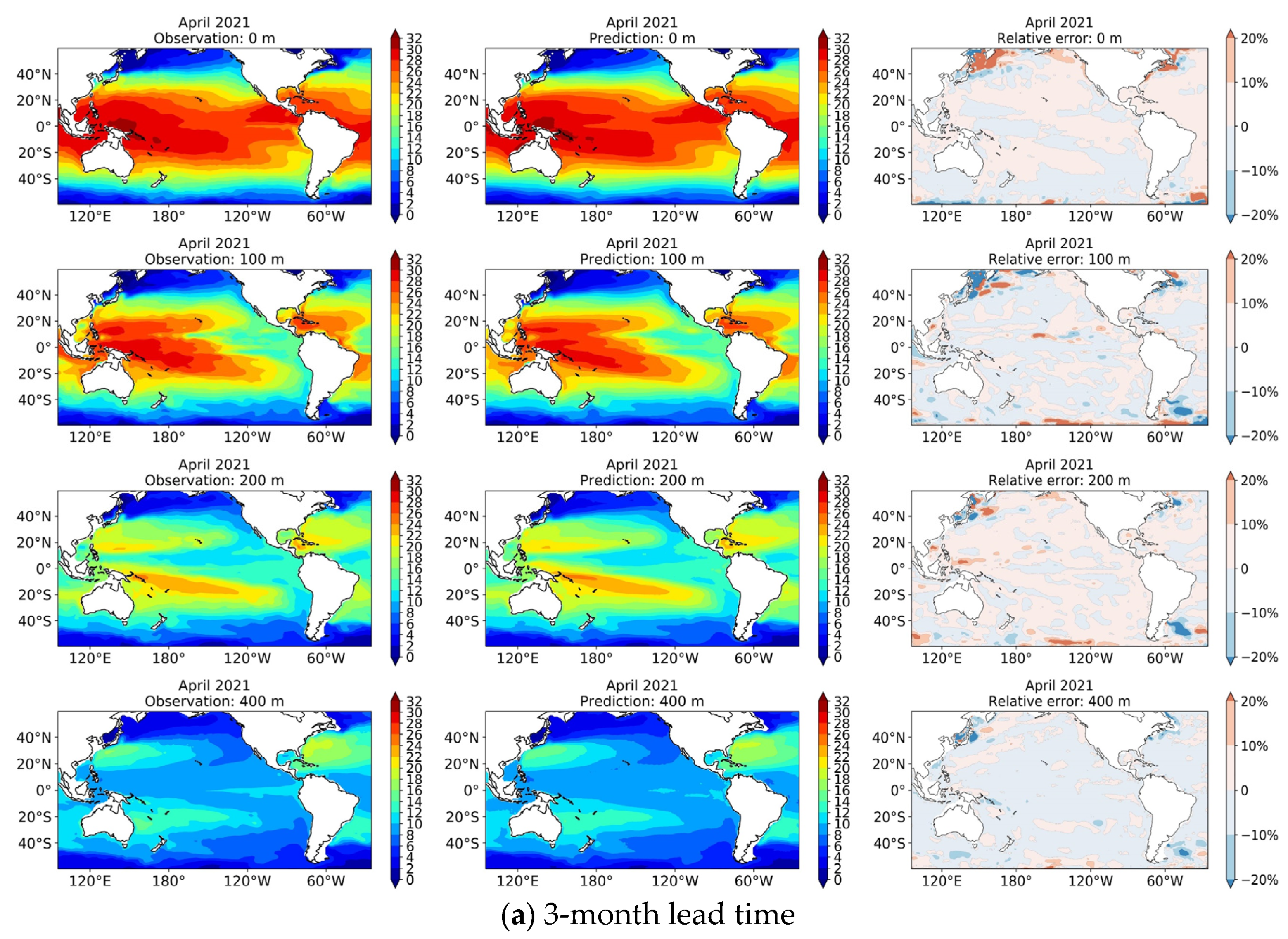
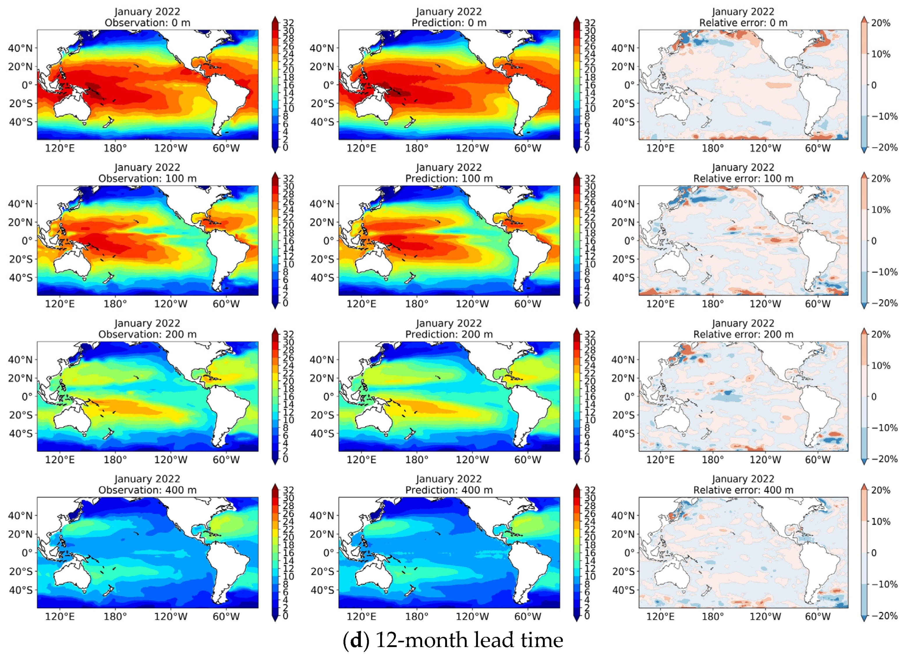
A case study was then conducted to qualitatively assess the 3D U-Net model’s performance in terms of prediction. The SSbT fields observed in the past 12 months from February 2020 to January 2021 were input into the model, and the prediction results for the next 12 months from February 2021 to January 2022 were obtained. Figure 8a–d show the prediction results for the lead times of 3, 6, 9, and 12 months together with the associated ground truth SSbT fields for the selected depths of 0, 100, 200, and 400 m. Maps of the relative error between the predictions and observations are also displayed. The SST shows an obvious seasonal variation, and the prediction results of the network well reflect this temporal characteristic. The distribution of the predicted sea temperature is comparable to that of the ground truth observations in the other three depth layers. In addition, the relative error in most regions is less than 10%. However, large relative error of more than 20% is found in temperate zones, mainly at the boundary of the study area and the regions close to the land. This may be due to the lack of utilization of temperature outside the study area and the complexity of SSbT variations in coastal seas. In general, the 3D U-Net model can predict realistic SSbT variations in the study area.

6. Conclusions

This study attempts to predict the SSbT over the Pacific Ocean and its surrounding oceans in the upcoming 12 months. We designed a 3D U-Net model to extract the spatiotemporal correlation of the input SSbT fields in the past 12 months and map them to the prediction results. The issue of insufficient training data was resolved using the reconstructed SSbT data. The experimental results indicate that after using additional reconstruction data, relative improvements of 7.5% and 9.3% are achieved in terms of RMSE and MAE, and a higher average CC value is obtained. The prediction of 50–150 m SSbT is more difficult than that at other depths, possibly because the inter-annual variations and vertical temperature gradients at these layers are larger than those at other layers. In addition, the SSbT prediction performance of the 3D U-Net model varies across different geographical parts of the study area. For the prediction of SST, the model has the lowest prediction error in tropics, while for the prediction of mesosphere temperature, the model has the largest prediction error in the tropical region. The overall prediction performance for SSbT in the Southern Hemisphere is better than that in the Northern Hemisphere, and the model performance in subtropical zones are better than that in temperate zones. The prediction error of this method is lower at most depth levels compared with that of other methods. It achieves better overall and longer-term prediction performance. The RMSE and MAE of the predicted SSbT fields for all lead times are in the range 0.5–0.7 °C and 0.3–0.45 °C, respectively, and the average CC scores of the predicted SSbT profiles exceed 0.96 for almost all lead times. A prediction case starting from January 2021 over the study area demonstrates that the 3D U-Net model is capable of simulating the temporal variations of the SSbT fields, and its predictions were in line with the observations, which can facilitate understanding of future changes in the thermal state of the subsurface ocean.
However, there is still a problem of input information loss in the 3D U-Net model, which makes its prediction accuracy for 400 m and the CC values of the predicted sea temperature profiles inferior to those of the seasonal naïve model. In the future, we will try to address this problem and incorporate more oceanic parameters such as ocean currents into the network to further improve the SSbT prediction performance.

Author Contributions

Conceptualization, N.S. and Q.L.; methodology, N.S.; software, N.S.; validation, N.S., Q.L., Z.Z. and X.Z.; formal analysis, N.S.; investigation, N.S.; resources, Q.L.; data curation, N.S.; writing—original draft preparation, N.S.; writing—review and editing, Q.L. and Z.Z.; visualization, N.S.; supervision, Q.L., Z.Z. and X.Z.; project administration, Q.L.; funding acquisition, Q.L. All authors have read and agreed to the published version of the manuscript.

Funding

This research was funded by the National Natural Science Foundation of China (Grant No. 42075139, 41305138), the China Postdoctoral Science Foundation (Grant No. 2017M621700), Hunan Province Natural Science Foundation (Grant No. 2021JJ30773), and Fengyun Application Pioneering Project (FY-APP).

Data Availability Statement

The IAP-reconstructed historical SSbT data can be downloaded from http://www.ocean.iap.ac.cn/ftp/cheng/CZ16_v3_IAP_Temperature_gridded_1month_netcdf/ (accessed on 4 July 2022); the RDA-reconstructed historical SSbT data are available from https://rda.ucar.edu/datasets/ds285.3/ (accessed on 4 July 2022); and the NOAA Optimum Interpolation (OI) SST V2 data and NCEP Global Ocean Data Assimilation System (GODAS) data are provided by the NOAA PSL, Boulder, Colorado, USA, from their website at https://psl.noaa.gov (accessed on 4 July 2022).

Acknowledgments

The authors would like to thank the anonymous reviewers for providing professional and insightful comments on the previous article. We offer our deepest thanks to the data contributors for sharing their data freely.

Conflicts of Interest

The authors declare no conflict of interest.

References

  1. Wentz, F.J.; Gentemann, C.; Smith, D.; Chelton, D. Satellite measurements of sea surface temperature through clouds. Science 2000, 288, 847–850. [Google Scholar] [CrossRef] [PubMed]
  2. Yao, S.L.; Luo, J.J.; Huang, G.; Wang, P. Distinct global warming rates tied to multiple ocean surface temperature changes. Nat. Clim. Change 2017, 7, 486–491. [Google Scholar] [CrossRef]
  3. Kao, H.Y.; Yu, J.Y. Contrasting eastern-Pacific and central-Pacific types of ENSO. J. Clim. 2009, 22, 615–632. [Google Scholar] [CrossRef]
  4. Anderson, B.T. On the joint role of subtropical atmospheric variability and equatorial subsurface heat content anomalies in initiating the onset of ENSO events. J. Clim. 2007, 20, 1593–1599. [Google Scholar] [CrossRef]
  5. Cione, J.J.; Uhlhorn, E.W. Sea surface temperature variability in hurricanes: Implications with respect to intensity change. Mon. Weather. Rev. 2003, 131, 1783–1796. [Google Scholar] [CrossRef]
  6. Belkin, I.M. Rapid warming of large marine ecosystems. Prog. Oceanogr. 2009, 81, 207–213. [Google Scholar] [CrossRef]
  7. Gou, Y.; Zhang, T.; Liu, J.; Wei, L.; Cui, J.H. DeepOcean: A general deep learning framework for spatio-temporal ocean sensing data prediction. IEEE Access 2020, 8, 79192–79202. [Google Scholar] [CrossRef]
  8. Klemas, V. Fisheries applications of remote sensing: An overview. Fish. Res. 2013, 148, 124–136. [Google Scholar] [CrossRef]
  9. Barnston, A.G.; Glantz, M.H.; He, Y. Predictive skill of statistical and dynamical climate models in SST forecasts during the 1997–98 El Niño episode and the 1998 La Niña onset. Bull. Am. Meteorol. Soc. 1999, 80, 217–244. [Google Scholar] [CrossRef]
  10. Stockdale, T.N.; Balmaseda, M.A.; Vidard, A. Tropical Atlantic SST prediction with coupled ocean–atmosphere GCMs. J. Clim. 2006, 19, 6047–6061. [Google Scholar] [CrossRef]
  11. Johnson, S.J.; Stockdale, T.N.; Ferranti, L.; Balmaseda, M.A.; Molteni, F.; Magnusson, L.; Monge-Sanz, B.M. SEAS5: The new ECMWF seasonal forecast system. Geosci. Model Dev. 2019, 12, 1087–1117. [Google Scholar] [CrossRef]
  12. Kondrashov, D.; Kravtsov, S.; Robertson, A.W.; Ghil, M. A hierarchy of data-based ENSO models. J. Clim. 2005, 18, 4425–4444. [Google Scholar] [CrossRef]
  13. Shirvani, A.; Nazemosadat, S.M.J.; Kahya, E. Analyses of the Persian Gulf sea surface temperature: Prediction and detection of climate change signals. Arab. J. Geosci. 2015, 8, 2121–2130. [Google Scholar] [CrossRef]
  14. Lins, I.D.; Araujo, M.; das Chagas Moura, M.; Silva, M.A.; Droguett, E.L. Prediction of sea surface temperature in the tropical Atlantic by support vector machines. Comput. Stat. Data Anal. 2013, 61, 187–198. [Google Scholar] [CrossRef]
  15. Corchado, J.M.; Fyfe, C. Unsupervised neural method for temperature forecasting. Artif. Intell. Eng. 1999, 13, 351–357. [Google Scholar] [CrossRef]
  16. Wei, L.; Guan, L.; Qu, L. Prediction of sea surface temperature in the South China Sea by artificial neural networks. IEEE Geosci. Remote Sens. Lett. 2019, 17, 558–562. [Google Scholar] [CrossRef]
  17. Zhang, Q.; Wang, H.; Dong, J.; Zhong, G.; Sun, X. Prediction of sea surface temperature using long short-term memory. IEEE Geosci. Remote Sens. Lett. 2017, 14, 1745–1749. [Google Scholar] [CrossRef]
  18. Ham, Y.G.; Kim, J.H.; Luo, J.J. Deep learning for multi-year ENSO forecasts. Nature 2019, 573, 568–572. [Google Scholar] [CrossRef]
  19. Haghbin, M.; Sharafati, A.; Motta, D.; Al-Ansari, N.; Noghani, M.H.M. Applications of soft computing models for predicting sea surface temperature: A comprehensive review and assessment. Prog. Earth Planet. Sci. 2021, 8, 1–19. [Google Scholar] [CrossRef]
  20. Zhang, Z.; Pan, X.; Jiang, T.; Sui, B.; Liu, C.; Sun, W. Monthly and quarterly sea surface temperature prediction based on gated recurrent unit neural network. J. Mar. Sci. Eng. 2020, 8, 249. [Google Scholar] [CrossRef] [Green Version]
  21. Yang, Y.; Dong, J.; Sun, X.; Lima, E.; Mu, Q.; Wang, X. A CFCC-LSTM model for sea surface temperature prediction. IEEE Geosci. Remote Sens. Lett. 2017, 15, 207–211. [Google Scholar] [CrossRef]
  22. Shi, X.; Chen, Z.; Wang, H.; Yeung, D.Y.; Wong, W.K.; Woo, W.-C. Convolutional LSTM network: A machine learning approach for precipitation nowcasting. Adv. Neural Inf. Process. Syst. 2015, 28, 802–810. [Google Scholar]
  23. Xiao, C.; Chen, N.; Hu, C.; Wang, K.; Xu, Z.; Cai, Y.; Gong, J. A spatiotemporal deep learning model for sea surface temperature field prediction using time-series satellite data. Environ. Model. Softw. 2019, 120, 104502. [Google Scholar] [CrossRef]
  24. Gupta, M.; Kodamana, H.; Sandeep, S. Prediction of ENSO beyond spring predictability barrier using deep convolutional LSTM networks. IEEE Geosci. Remote Sens. Lett. 2020, 19, 1501205. [Google Scholar] [CrossRef]
  25. Zhang, K.; Geng, X.; Yan, X.H. Prediction of 3-D ocean temperature by multilayer convolutional LSTM. IEEE Geosci. Remote Sens. Lett. 2020, 17, 1303–1307. [Google Scholar] [CrossRef]
  26. Wu, X.; Yan, X.H.; Jo, Y.H.; Liu, W.T. Estimation of subsurface temperature anomaly in the North Atlantic using a self-organizing map neural network. J. Atmos. Ocean. Technol. 2012, 29, 1675–1688. [Google Scholar] [CrossRef]
  27. Cheng, L.; Zhu, J. Benefits of CMIP5 multimodel ensemble in reconstructing historical ocean subsurface temperature variations. J. Clim. 2016, 29, 5393–5416. [Google Scholar] [CrossRef]
  28. Liu, J.; Zhang, T.; Han, G.; Gou, Y. TD-LSTM: Temporal dependence-based LSTM networks for marine temperature prediction. Sensors 2018, 18, 3797. [Google Scholar] [CrossRef]
  29. Patil, K.R.; Iiyama, M. Deep Neural Networks to Predict Sub-surface Ocean Temperatures from Satellite-Derived Surface Ocean Parameters. In Soft Computing for Problem Solving; Springer: Singapore, 2021; pp. 423–434. [Google Scholar]
  30. Zuo, X.; Zhou, X.; Guo, D.; Li, S.; Liu, S.; Xu, C. Ocean temperature prediction based on stereo spatial and temporal 4-D convolution model. IEEE Geosci. Remote Sens. Lett. 2021, 19, 1–5. [Google Scholar] [CrossRef]
  31. Ishii, M.; Kimoto, M.; Sakamoto, K.; Iwasaki, S. Subsurface Temperature and Salinity Analyses; Research Data Archive at the National Center for Atmospheric Research. Accessed 4 June 2022; Computational and Information Systems Laboratory: Boulder, CO, USA, 2005. [Google Scholar] [CrossRef]
  32. Reynolds, R.W.; Rayner, N.A.; Smith, T.M.; Stokes, D.C.; Wang, W. An improved in situ and satellite SST analysis for climate. J. Clim. 2002, 15, 1609–1625. [Google Scholar] [CrossRef]
  33. Behringer, D.W.; Ji, M.; Leetmaa, A. An improved coupled model for ENSO prediction and implications for ocean initialization. Part I: The ocean data assimilation system. Mon. Weather. Rev. 1998, 126, 1013–1021. [Google Scholar] [CrossRef]
  34. Yang, K.; Cai, W.; Huang, G.; Wang, G.; Ng, B.; Li, S. Oceanic processes in ocean temperature products key to a realistic presentation of positive Indian Ocean Dipole nonlinearity. Geophys. Res. Lett. 2020, 47, e2020GL089396. [Google Scholar] [CrossRef]
  35. Tang, Y.; Duan, A. Using deep learning to predict the East Asian summer monsoon. Environ. Res. Lett. 2021, 16, 124006. [Google Scholar] [CrossRef]
  36. Çiçek, Ö.; Abdulkadir, A.; Lienkamp, S.S.; Brox, T.; Ronneberger, O. U-net: Learning dense volumetric segmentation from sparse annotation. In Proceedings of the International Conference on Medical Image Computing and Computer-Assisted Intervention, Athens, Greece, 17–21 October 2016; Springer: Cham, Switzerland, 2016; pp. 424–432. [Google Scholar]
  37. Ioffe, S.; Szegedy, C. Batch normalization: Accelerating deep network training by reducing internal covariate shift. In Proceedings of the International Conference on Machine Learning, Lille, France, 7–9 July 2015; pp. 448–456. [Google Scholar]
  38. Tran, D.; Bourdev, L.; Fergus, R.; Torresani, L.; Paluri, M. Learning spatiotemporal features with 3d convolutional networks. In Proceedings of the IEEE International Conference on Computer Vision, Santiago, Chile, 7–13 December 2015; pp. 4489–4497. [Google Scholar]
  39. Abadi, M.; Agarwal, A.; Barham, P.; Brevdo, E.; Chen, Z.; Citro, C.; Zheng, X. Tensorflow: Large-Scale Machine Learning on Heterogeneous Distributed Systems. arXiv 2016, arXiv:1603.04467. [Google Scholar]
  40. Doney, S.; Yeager, S.; Danabasoglu, G.; Large, W.; McWilliams, J. Modeling Global Oceanic Interannual Variability (1958–1997): Simulation Design and Model-Data Evaluation; Tech. Note NCAR/TN-452+ STR; National Center for Atmospheric Research: Boulder, CO, USA, 2003. [Google Scholar]
  41. Zhang, Y.; Li, K.; Li, K.; Wang, L.; Zhong, B.; Fu, Y. Image super-resolution using very deep residual channel attention networks. In Proceedings of the European Conference on Computer Vision (ECCV), Munich, Germany, 8–14 September 2018; pp. 286–301. [Google Scholar]
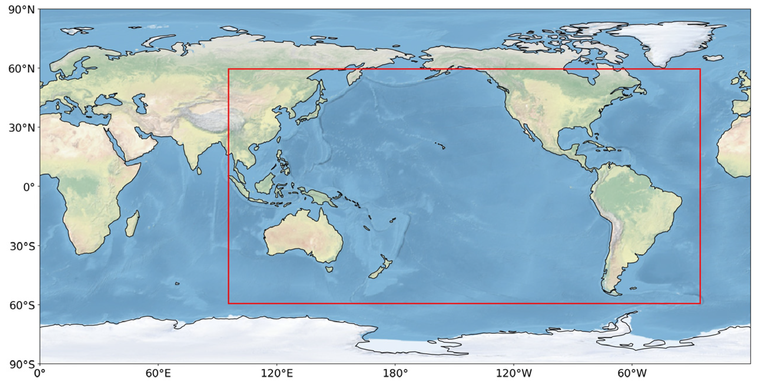
Figure 1. Selected study area.
Remotesensing 14 04890 g001
Figure 2. The architecture of the proposed model. k and s indicate the size and stride of convolution kernels, respectively.
Remotesensing 14 04890 g002
Figure 3. RMSE loss against epochs for the 3D U-Net model.
Remotesensing 14 04890 g003
Figure 4. RMSE (a) and MAE (b) of the prediction results at different depth levels for selected lead times (LTs).
Remotesensing 14 04890 g004
Figure 5. Average root-mean-square (RMS) temperature variations (a) and average vertical temperature gradients (b) at different depth levels in the study area.
Remotesensing 14 04890 g005
Figure 6. RMSE curves of the compared methods against lead times of 1–12 months for selected depth levels.
Remotesensing 14 04890 g006
Figure 7. Evaluation of the overall prediction performance of different models.
Remotesensing 14 04890 g007
Figure 8. A prediction case starting from January 2021 for lead times of 3 (a), 6 (b), 9 (c), and 12 (d) months. In each subfigure, from left to right are the observations, prediction results, and maps of the relative error between them, and from top to bottom, subfigures correspond to depth levels of 0, 100, 200, and 400 m.
Remotesensing 14 04890 g008aRemotesensing 14 04890 g008bRemotesensing 14 04890 g008c
Table 1. Organization of the built dataset.
SubsetProductPeriodNumber of Sequences
TrainingIAPJanuary 1956–December 20071623
RDAJanuary 1945–December 2007
OISST V2 and GODASJanuary 1982–December 2007
ValidationOISST V2 and GODASJanuary 2008–December 201260
TestOISST V2 and GODASJanuary 2013–May 2022102
Table 2. The effect of adding reconstruction data during model training.
DatasetRMSEMAECC
Observation data0.68570.42270.9506
Reconstructed data + observation data0.63430.38320.9616
Table 3. RMSE values of the predicted SSbT for selected depth levels over different geographical zones.
DepthNorth TemperateNorth SubtropicsTropicsSouth SubtropicsSouth Temperate
00.73230.62000.53630.54680.5876
200.71940.58110.60030.46480.5256
500.77540.63340.92590.45680.5182
1000.64940.61091.06860.44240.5179
2000.51630.46570.64880.43760.4540
4000.41800.41230.39240.34070.3147
Table 4. Evaluation of the overall prediction performance for the SSbT fields in different geographical zones.
RegionRMSEMAECC
North temperate0.63910.33300.9177
North subtropics0.55650.37180.9935
Tropics0.73450.44540.9960
South subtropics0.44920.31300.9955
South temperate0.48930.34990.9081
Publisher’s Note: MDPI stays neutral with regard to jurisdictional claims in published maps and institutional affiliations.