Detection and Counting of Corn Plants in the Presence of Weeds with Convolutional Neural Networks

Abstract

Corn is an important part of the Mexican diet. The crop requires constant monitoring to ensure production. For this, plant density is often used as an indicator of crop yield, since knowing the number of plants helps growers to manage and control their plots. In this context, it is necessary to detect and count corn plants. Therefore, a database of aerial RGB images of a corn crop in weedy conditions was created to implement and evaluate deep learning algorithms. Ten flight missions were conducted, six with a ground sampling distance (GSD) of 0.33 cm/pixel at vegetative stages from V3 to V7 and four with a GSD of 1.00 cm/pixel for vegetative stages V6, V7 and V8. The detectors compared were YOLOv4, YOLOv4-tiny, YOLOv4-tiny-3l, and YOLOv5 versions s, m and l. Each detector was evaluated at intersection over union (IoU) thresholds of 0.25, 0.50 and 0.75 at confidence intervals of 0.05. A strong F1-Score penalty was observed at the IoU threshold of 0.75 and there was a 4.92% increase in all models for an IoU threshold of 0.25 compared to 0.50. For confidence levels above 0.35, YOLOv4 shows greater robustness in detection compared to the other models. Considering the mode of 0.3 for the confidence level that maximizes the F1-Score metric and the IoU threshold of 0.25 in all models, YOLOv5-s obtained a mAP of 73.1% with a coefficient of determination ($R^2$) of 0.78 and a relative mean square error (rRMSE) of 42% in the plant count, followed by YOLOv4 with a mAP of 72.0%, $R^2$ of 0.81 and rRMSE of 39.5%.

1. Introduction

Corn (Zea mays L.) production in Mexico for the year 2020 exceeded 27.4 million tons [1]. Corn is one of the most important crops in the country from a food, political, economic and social perspective [2]. Cereals form a crucial part of the human diet and livestock feed, so achieving self-sufficiency in their production is an effective way to promote food security [3].

Knowing the number of plants and monitoring their growth status are important for estimating yield [4,5]. Manual counting after plant emergence is not practical in large-scale production fields due to the amount of labor required, in addition to which it is inherently inaccurate [3,4,6]. One approach that has been applied in recent years is the use of remotely piloted aerial systems (RPAS) equipped with optical sensors for agricultural remote sensing [7]. Several studies have reported on the use of RPAS to determine planting densities in different crops; for example, in [8], they reported on its use for the detection of cotton plants, based on machine learning with convolutional neural networks (CNNs), in [9], they used CNNs for the detection and counting of tobacco plants, in [10], they propose a CNN (WheatNet) based on MobileNetV2 with two outputs for the localization and counting of wheat ears from images; similarly, in [11], they propose an integrated image pre-processing method (Excess Green Index and Otsu’s method) and CNNs for identifying and counting spinach plants.

Three methods for counting and classifying corn plants have been reported in the literature:

(1) Classical image processing techniques. In [12], RGB cameras mounted on RPAS were compared using templates and normalized cross-correlation, obtaining $R^2$ coefficients of 0.98, 0.90 and 0.16 for vegetative stages V2, V5 and V9, respectively. Gnädinger and Schmidhalter [13], using the decorrstrech contrast enhancement procedure with thresholding, obtained $R^2$ coefficients of 0.89 for vegetative stages V3 and V5. Shuai et al. [14] employed the excess green (ExG) vegetation index, achieving a precision of 95% and recall of 100% for plant counts at vegetative stage V2.

(2) Classical image processing techniques plus machine learning procedures. In [15], they used principal component analysis (PCA) and Otsu’s thresholding method to extract features as input to Naive Bayes neural network and Random Forest classifiers to classify corn plants and weeds in images captured with mobile devices. Varela et al. [6] used color indices, geometric descriptors and decision tree classifiers for corn counting, achieving accuracies of 96% for stages V2 and V3. Pang et al. [16] combined geometric descriptors and convolutional neural networks to count corn plants, achieving accuracies of 95.8% for vegetative stages V5 and V4.

(3) Machine learning with CNNs. In [17], they compared color indices with CNN architectures, specifically “You Only Look Once” (YOLO) in its YOLOv3 and YOLOv3-tiny versions, to evaluate the detection of corn plants in images captured at a height of 0.3 m from the ground, achieving a 77% intersection over union (IoU). Wan et al. [18] used a robot-mounted camera for real-time plant detection and counting, employing YOLOv3 and a Kalman filter, and achieved accuracies of 98% at stages V2 and V3. Vong et al. [19] performed semantic segmentation with the U-NET architecture, obtaining $R^2$ coefficients of 0.95 at the V2 stage. Velumani et al. [20] evaluated the performance of Faster-RCNN for corn plant counting at different spatial resolutions, achieving an rRMSE value of 8% with a ground sampling distance (GSD) of 0.3 cm/pixel. Osco et al. [5] proposed a CNN-based architecture for segmenting and counting corn plants, achieving F1-Scores of 0.87 for stage V3. Etienne et al. [21] compared classical methods for image processing and Faster-RCNN in counting corn, sugar beet and sunflower plants.

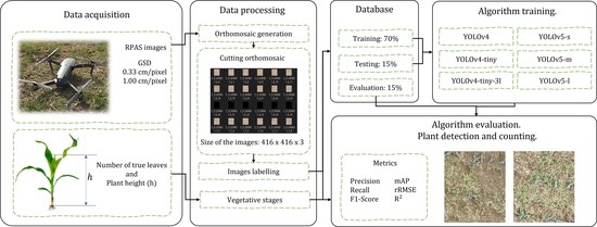
In general, the best results were obtained when using CNNs with deep learning methods. Although there are some works that analyze the effects of weeds on the detection and counting of corn plants in aerial images [5,15,21], given the complexity of possible scenarios and the conditions of corn fields in Mexico, labeled databases are still required to assess the robustness of state-of-the-art object detection algorithms. Therefore, the following contributions are made in this paper: (i) a database with 11,191 aerial images of dimension 416 × 416 × 3 labeled, (ii) a comparison of the results obtained by YOLOv4, YOLOv4-tiny, YOLOv4-tiny-3l, YOLOv5-s, YOLOv5-m and YOLOv5-l models in the detection and counting of corn plants in weed-infested fields, considering the value of the intersection over union and confidence and (iii) the optimization of the confidence level and the intersection over union that maximize the F1-Score metric in the evaluation of the models.

The paper is organized as follows. Section 2.1 describes the conditions and the process used for the acquisition of aerial images, as well as the labeling process for the formation of the database; Section 2.2 and Section 2.3 describes the algorithms used and the evaluation metrics. The results and discussion are provided in Section 3 and Section 4, respectively. Finally, Section 5 provides conclusions and offers ideas for future research.

2. Materials and Methods

2.1. Dataset

The research area was divided into five experimental sites, located at the Universidad Autónoma Chapingo, Texcoco, State of Mexico, geographically located at: 19°29’27.3″N Lat., 98°53’06.9″W Long., and 2260 m a.s.l. For easy identification, the experimental fields were named Irrigación, Xerona, San Juan A1, San Juan A2 and Ranchito X13 (Figure 1). All experimental sites had the hybrid corn variety CP-HS2 except for the Ranchito X13 site, which had multiple varieties intended for breeding purposes.

Table 1. Data capture areas.

Experimental Sites	Geographic Coordinates		Variety	Planting
	Latitude	Longitude		Arrangement
Irrigación	19° 28’28″W	98° 53’28″W	Hybrid CP-HS2	1 Row
Xerona	19° 29’02″N	98° 53’57″W	Hybrid CP-HS2	2 Rows
San Juan A1	19° 29’32″N	98° 51’38″W	Hybrid CP-HS2	1 Row
San Juan A2	19° 29’31″N	98° 51’34″W	Hybrid CP-HS2	1 Row
Ranchito X13	19° 29’36″N	98° 52’43″W	Varied a	1 Row

^a More than one variety in the same area.

describes the planting arrangement, variety and geographic coordinates for each experimental site.

2.1.1. Data Acquisition

In addition to image acquisition, samples of the number of leaves and the height of the corn plant were taken. Aerial images were acquired using a DJI Mavic Pro multirotor RPAS (SZ DJI Technology Co., Shenzhen, Guangdong, China), equipped with an FC220 model RGB camera, with the following features:

• 1/2.3″ CMOS sensor with 12.7 M total pixels and 12.3 M effective pixels;
• FOV 78.8° 26 mm lens;
• 2.22 mm focal length;
• Distortion < 1.5%;
• ISO range from 100 to 1600;
• Image size: 4000 × 3000 pixels;
• 8 s–1/8000 s shutter speed.

Flight missions were planned and carried out from 10:00 a.m. to 2:00 p.m., with an overlap between images of 80%, both frontal and lateral, and a nadir-pointing camera view. The RPAS flight altitude was 10 m for a GSD of 0.33 cm/pixel and 30 m for a GSD of 1.00 cm/pixel.

Table 2. Characteristics of flight missions.

Data of Capture	GSD (cm/pixel)	Area (m${}^2$)	Captured Images	Temperature (°C)	Wind Speed (km/h)	Visibility (km)
Irrigación
2 August 2021	0.33	2883	479	23	7.41	6.7
9 August 2021		3564	438	18	9.26	11.3
18 August 2021		3722	436	23	13.00	8
26 August 2021		1950	466	23	7.41	16.1
Xerona
8 July 2021	0.33	1663	293	16	7.56	9.66
8 July 2021	1.00	16,106	360	16	7.56	9.66
14 July 2021	0.33	1667	294	14	5.4	6.66
San Juan A1
17 June 2021	1.00	15,177	361	16	13	12.9
San Juan A2
1 July 2021	1.00	11,281	222	17	7.56	11.3
Ranchito X13
24 June 2021	1.00	10,696	306	19	7.41	4.84

summarizes the flight missions, sampled area, captured images and weather conditions.

To define the state of the crop, 30 random samples of the number of leaves and plant height were obtained during each flight mission, determining the vegetative stage expressed with the letter V plus the number of true leaves, following the methodology described in [22], and the average height of the corn plants. As in [21], weed infestation was qualitatively determined by assigning values of 0, 1 and 2 for weed-free areas, low weed presence and weed infestation, respectively. Subscripts F, P and T were included to locate weeds between rows, between plants and total cover (

Table 3. Crop characterization.

Date of Capture	Days after Planting	Vegetative Stage	Average Plant Height (cm)	Weed Infestation
Irrigación
2 August 2021	16	V3	9.62 ± 1.66	$1_T$
9 August 2021	23	V4	16.8 ± 4.39	$2_T$
18 August 2021	32	V5	25.16 ± 6.00	$2_T$
26 August 2021	40	V6	34.68 ± 8.00	$1_T$
Xerona
8 July 2021	44	V6	52.94 ± 6.64	$0_F,2_P$
8 August 2021	44	V6	52.94 ± 6.64	$0_F,2_P$
14 July 2021	50	V7	75.68 ± 10.43	$0_F,2_P$
San Juan A1
17 June 2021	57	V7	49.86 ± 10.39	$0_T$
San Juan A2
1 July 2021	71	V8	92.94 ± 21.67	$2_T$
Ranchito X13
24 June 2021	59	V7	75.78 ± 18.41	$0_T$

).

2.1.2. Plant Labeling

Pix4D mapper software (Pix4D SA, Lausanne, Switzerland) was used in the orthorectification of the images, obtaining the best results with the following parameter settings: in the initial process for the extraction of key points, the full image, alternative calibration and internal parameter optimization with high priority were used. For the generation of the point cloud and the mesh, half of the image was used.

For each flight mission, an orthomosaic was obtained and divided into 416 × 416 pixel images to form the corn plant database. The manual labeling of the plants (ground truth label) was performed with the LabelImg tool [23], respecting the format required by YOLO. Each label corresponds to the group of pixels in RGB belonging to a corn plant, assigned the name “MAIZ,” the Spanish word for corn. In the labeling process, the following considerations were taken into account: (1) the box of each label covered the whole plant, (2) in case of incomplete plants at the edges of the image, blurred plants and plants with ghost leaves, labels were considered correct only if the center of the plant was completely visible, and (3) images with errors in their stitching or too much complexity in the labeling were eliminated. Examples of labeling and weed infestation conditions at different vegetative stages with different ground sampling distances are shown in Figure 2a–f.

2.1.3. Database Description

The database is composed of images with a size of 416 × 416 pixels, obtained completely at random from each orthomosaic with the proportion of 70% for training, 15% for testing and 15% for evaluation, making a total of 11,191 images and 85,419 labels. Considering each vegetative stage and its GSD spatial resolution in cm/pixel, Figure 3 shows the distribution of corresponding images for training, testing and evaluation.

According to the definitions of [24] and the COCO database [25] regarding the size of the labels, they were grouped into small (area < ${32}^2$ pixels), medium-sized (${32}^2$ < area < ${96}^2$ pixels) and large (area > ${96}^2$ pixels) categories. Figure 4 shows the size distribution of the labels in the database, where 35.58% of the labels are small, 59.58% medium-sized and 4.48% large.

2.2. Detection Algorithms and Their Training

A convolutional neural network (CNN) is a variant of the multilayer perceptron (MLP) architecture, inspired by the animal visual cortex and designed for image processing, based on three main types of neural layers: convolutional layers that apply 2D convolution operations to find different features of interest in an image; downsampling layers that reduce the spatial dimension of the convolutional layers and fully connected layers (MLP) that handle high-level inference in the network [26,27]. Automatic feature extraction through convolutional filter optimization gives CNNs a competitive advantage over traditional algorithms.

Object detection using CNNs combines image classification and object localization. Generally, they are based on region proposals and the classification of each region into different categories or as a regression/classification problem. Generally, these algorithms fall into two broad categories: two-stage detectors that perform object location based on the proposal of regions and then are classified into different categories, and detectors that directly determine the location and classification of objects in a single step based on regression/classification [28].

Analyzing the results obtained by [29], when comparing different CNNs architectures in object detection and considering the proposal of [20], the YOLOv4 [30] and YOLOv5 [31] architectures were selected as the basis for this research work. These versions of YOLO [32] are mainly composed of three parts: feature extractor (Backbone), feature aggregation for detection at different scales (Neck) and prediction/regression (Head); the difference between these YOLO variants is based on the modification of these three parts, such as changes in the loss function, activation function, and regularization techniques, among others.

The YOLOv4 model uses CSPNet + Darknet53 architectures previously trained with the ImageNet database for feature extraction, SSP + PANet for feature aggregation and the proposed YOLOv3 regression/classification [33] for object detection [34]. Figure 5 shows the diagram corresponding to the YOLOv4 architecture with an input image of size 416 × 416 × 3 and three prediction heads at different scales with 3 boxes each, obtaining a tensor N × N × [3 × (4 bounding box offsets + 1 objectness prediction + n_classes)].

Following the full version of YOLOv4, the versions YOLOv4-tiny with two prediction outputs at different scales and YOLOv4-tiny-3l with three outputs were derived, keeping a reduced number of layers from its original version. Figure 6 shows the diagram of the YOLOv4-tiny-3l architecture; in our case, for the YOLOv4-tiny version, the 52 × 52 × 18 output was removed.

The YOLOv4-tiny version was selected because it has faster inference times and the YOLOv4-tiny-3l version because it was expected to provide better results than YOLOv4-tiny due to its having one more output at similar inference times. In the same way as YOLOv4, the implementation of YOLOv5 presents versions n, s, m, l and x with different accuracy and detection speeds [28]; therefore, the s, m and l versions were implemented.

Like YOLOv4, YOLOv5 is based on the architectures of CSPNet + Darknet53 (backbone), SSP + PANet (neck), and YOLOv3 Head for object detection. The latest changes in the architecture (V6.0/6.1) are in the first layer FOCUS by the CBS equivalent with inputs $[N_{Kernels}=64,Kernel=6,Stride=2,Padding=2]$ and SPP by an equivalent called SPPF, improving the training and inference times of the network.

The structure for all YOLOv5 variants is maintained (Figure 7); only the width and depth of the network are modified.

The modification of the network depth was carried out by taking the positive integer of the multiplication of the B_Neck blocks by a factor and the width of the network by multiplying the number of filters by a factor, as shown in

Table 4. YOLOv5 versions.

Version	Depth of Architecture	Layer Width
YOLOv5-n	0.33	0.25
YOLOv5-s	0.33	0.50
YOLOv5-m	0.67	0.75
YOLOv5-l	1.00	1.00
YOLOv5-x	1.25	1.25

.

The implementation of YOLOv4 was based on the darknet framework written in the C programming language and YOLOv5 on the Pytorch library implemented in Python, both open-source tools. To train of the algorithms, the hyperparameters proposed in each implementation of each CNN optimized for the COCO database were used, and are described in detail in

Table 5. Algorithm training hyperparameters.

Algorithm	Image Size	Batch	Optimizer	Learning Rate	Decay (% Iterations)	Iterations	Pre-Training Weights
YOLOv4	416 × 416 × 3	64	SGD	0.0013	25, 80 and 90	10,000	COCO
YOLOv4-tiny		64	SGD	0.00261	80 and 90	20,000	COCO
YOLOv4-tiny-3l		64	SGD	0.00261	80 and 90	20,000	COCO
YOLOv5-s		179	Adam	0.01	Automatic	200	COCO
YOLOv5-m		99	Adam	0.01	Automatic	200	COCO
YOLOv5-l		179	Adam	0.01	Automatic	200	COCO

.

2.3. Evaluation Metrics

The metrics precision (Pr), recall (Rc), mean average precision (mAP) and F1-Score, commonly used to evaluate the results in object detection work [35], were employed. As only one class was considered, the mAP was equal to average precision (AP). The AP calculation was performed using the so-called all-point interpolation (APall) [35], adopted in the Pascal Challenge [36].

Pr is the percentage of correct positive predictions [35].

$$\mathrm{Pr}=\frac{\mathrm{TP}}{\mathrm{TP}+\mathrm{FP}},$$

(1)

Rc is the percentage of correct positive predictions among all given ground truths [35].

$$\mathrm{Rc}=\frac{\mathrm{TP}}{\mathrm{TP}+\mathrm{FN}},$$

(2)

where:

• TP (True positive): a correct detection of a ground-truth bounding box if its area of intersection over the area of union (IoU) with the corresponding labeled bounding box is greater than a given threshold.
• FP (False positive): an incorrect detection of a non-existing object or a misplaced detection of an existing object.
• FN (False negative): an undetected ground-truth bounding box.

The F1-Score is defined as the harmonic mean of the precision and recall of a given detector.

$$\mathrm{F}1\text{-}\mathrm{Score}=2\ast \frac{\mathrm{Pr}\ast \mathrm{Rc}}{\mathrm{Pr}+\mathrm{Rc}},$$

(3)

To determine the above metrics, an open source software developed by [35] was used and the source code was modified to evaluate all the proposed CNN models.

To measure the counting performance of the models, we used the coefficient of determination ($R^2$) [37] and the relative root mean square error (rRMSE) proposed in [21], where an rRMSE < 5% is considered good, satisfactory between 5% < rRMSE < 10%, poor between 10% < rRMSE < 20% and very poor rRMSE > 20%.

3. Results

3.1. Training

The training process of the neural algorithms was performed offline, using the services of Google Colab, which provides a virtual environment with a Graphics Processing Unit (GPU).

Table 6. Training time for each neural algorithm.

Algorithm	GPU	Training Time (Hours)	N Iterations
YOLOv4	Tesla T4-15 GB	27.40	10,000
YOLOv4-tiny	Tesla P100-PCIE-16 GB	4.70	20,000
YOLOv4-tiny-3l	Tesla T4-15 GB	7.90	20,000
YOLOv5-s	Tesla P100-PCIE-16 GB	3.60	200
YOLOv5-m	Tesla P100-PCIE-16 GB	10.00	200
YOLOv5-l	Tesla T4-15 GB	7.16	145

shows the training duration in hours, number of iterations and the GPU assigned to each trained model.

Figure 8 shows the behavior of the mAP metric for each model in the test dataset during the training. It can be seen that, for the YOLOv4 network, the mAP remained at values of 73% after iteration 2500, with no significant improvement in subsequent iterations. In the case of the YOLOv4-tiny and YOLOv4-tiny-3l models, the mAP value remained in the range from 60% to 65% until 16,000 iterations, reaching maximum values of 68% and 69% after applying a decay in the learning rate. For the YOLOv5-s and YOLOv5-m versions, the mAP was stable after epoch 75 and increased slightly in later epochs. For YOLOv5-l, the mAP values stabilized and increased until epoch 75, where learning remained constant and, as there was no further improvement, the process stopped at epoch 145.

The maximum [email protected] score in the test dataset was obtained by the YOLOv5-s model with a value of 77.6% and F1-Score of 73.0%, followed by the YOLOv5-m model. Although the YOLOv4 model is better in terms of the Rc metric, with a value of 77%, it obtained a low Pr, which penalizes the F1-Score and mAP.

Table 7. Test set metrics for a confidence of 0.25 and IoU of 0.50.

Model	Pr	Rc	F1-Score	[email protected]
YOLOv4	0.650	0.770	0.700	0.736
YOLOv4-tiny	0.620	0.730	0.670	0.686
YOLOv4-tiny-3l	0.680	0.670	0.670	0.691
YOLOv5-s	0.720	0.742	0.730	0.776
YOLOv5-m	0.700	0.748	0.723	0.769
YOLOv5-l	0.683	0.725	0.703	0.740

shows the Pr, Rc, F1-Score and mAP metrics obtained by each model in the test dataset in more detail.

3.2. Evaluation

The F1-Score for each CNN was determined at IoU threshold values of 0.25, 0.50 and 0.75, for confidence values in the range from 0.05 to 1.00 in intervals of 0.05, obtaining the results shown in Figure 9 for the evaluation data. The maximum F1-Scores were obtained at the same confidence values for an IoU threshold of 0.50 and 0.25, with an average increase of 4.92% for each model when going from IoU threshold of 0.50 to 0.25.

Figure 10a,b show an example of the impact on TP and FP when evaluating YOLOv5-l with IoU thresholds of 0.5 and 0.25. These images belong to stage V4 with GSD of 0.33 cm/pixel.

Table 8. Results for each model obtained in the evaluation dataset.

Model	Pr	Rc	F1-Score	mAP	TP	FP	FN	rRMSE	${\mathit{R}}^2$
YOLOv4	0.7057	0.8078	0.7533	0.7201	0.8078	0.3368	0.1921	0.3955	0.8116
YOLOv4-tiny	0.7049	0.7460	0.7249	0.6491	0.7460	0.3122	0.2539	0.4869	0.7114
YOLOv4-tiny-3l	0.7700	0.6489	0.7042	0.5806	0.6489	0.1938	0.3510	0.6384	0.4970
YOLOv5-s	0.7695	0.7937	0.7814	0.7310	0.7937	0.2374	0.2062	0.4206	0.7857
YOLOv5-m	0.7770	0.7751	0.7761	0.7160	0.7751	0.2223	0.2248	0.4614	0.7426
YOLOv5-l	0.7637	0.7477	0.7557	0.6853	0.7477	0.2312	0.2522	0.5349	0.6542

shows the results for the Pr, Rc, F1-Score, mAP, rRMSE and $R^2$ metrics for each evaluated CNN model. TP, FP and FN values are shown normalized from 0 to 1 and FP is expressed relative to the sum of TP + FN. The highest F1-Scores were obtained with the YOLOv5-s and YOLOv5-m models, with values of 0.7814 and 0.776, respectively. Regarding the Rc metric, the YOLOv4 model outperformed the other models, with a value of 80.78%, followed by YOLOv5-s, with a value of 79.37%. In terms of plant counts, the YOLOv4 model had the highest correlation with $R^2$ of 0.81 and rRMSE of 39.55%, followed by the YOLOv5-s model with $R^2$ of 0.78 and rRMSE of 42.06%.

In order to analyze the values obtained in Table 8, recall vs. precision curves were plotted for each of the vegetative stages with their spatial resolution; these results are shown in Figure 11. For stages $V{3}_{0.33}$ and $V{4}_{0.33}$, the models behaved consistently with Pr values between 77% and 85%, and Rc above 90%, except for the YOLOv4-tiny-3l model, in which it decayed to a value of 85%. The YOLOv4 model and YOLOv5 versions maintained the results of 70% < Pr < 80% and 85% < Rc < 90% for vegetative stages $V{5}_{0.33}$, $V{6}_{0.33}$ and $V{7}_{0.33}$, where the highest score was obtained at stage $V{5}_{0.33}$, followed by $V{7}_{0.33}$.

Comparing the estimation of the number of plants per image for each model, the rRMSE was obtained, Figure 12. The best results were obtained at vegetative stages V3, V4 and V5 with a GSD of 0.33 cm/pixel with rRMSE values between 10 and 20%, an error that increases at vegetative stages higher than V5.

The $R^2$ coefficient determines the relationship between the real plants and the number of plants estimated by the network, considering a confidence of 0.3 and an IoU threshold of 0.25; values higher than 0.85 were obtained with the YOLOv4 model, for vegetative stages V3, V4, V5, V6 and V7 with a GSD of 0.33 cm/pixel. Figure 13 shows the results obtained for each of the CNN architectures in more detail.

The detections were visually inspected for errors. It was observed that TPs at vegetative stages V3, V4 and V5 with a GSD of 0.33 cm/pixel were mainly caused by corn plant leaves at the edges of the image, and, in some cases, at V3, they were mistaken for weeds, as shown in Figure 14a. For vegetative stages after V5 and a GSD of 1.00 cm/pixel, it was observed that the FPs were mainly due to a lack of labels, since they were not due to the complexity of manual labeling, as shown in Figure 14b–d.

4. Discussion

The confidence value for the evaluation was chosen with the mode. When the models reached the maximum F1-Score, this value of 0.3 is lower than that of [20], who report a confidence of 0.5 when evaluating the Faster-RCNN architecture, indicating better results in terms of plant classification. YOLOv4-based models with confidence values higher than 0.35 maintain a higher F1-Score value than YOLOv5 versions, indicating that YOLOv4 models are more reliable in terms of classifying corn plants.

Most of the works on object detection in large datasets evaluate CNN models at IoU thresholds higher than 0.5 [35]. By analyzing the graphs in Figure 9, considering IoU thresholds greater than 0.5, a decrease can be seen in the F1-Score metric, indicating that the models lose precision in estimating the size of the corn plant. This can be seen in Figure 14a, where it is observed that, in some cases, the label prediction does not include the plant leaves, and since the IoU threshold of 0.5 is not exceeded, they would be considered FP predictions. As in [20], the F1-Score metric was evaluated at an IoU threshold of 0.25. An average increase of 4.92% was achieved for all YOLO models from an IoU threshold of 0.50. For the purposes of plant counting and detection, accurate estimation of plant dimensions is not considered critical [20]. Consequently, the IoU threshold value of 0.25 and a confidence of 0.3 were used to better account for the smaller size of the detected bounding boxes and the classification of corn plants, as was done in [20].

With respect to the plant count, YOLOv4 has a higher number of TPs, so it correlates better with the actual number of plants, with $R^2$ = 0.81 and rRMSE = 39.55%, followed by the YOLOv5-s model, with $R^2$ = 0.78 and rRMSE = 42.06%. Although there is a high correlation with the actual number of plants in both models, according to [21], they would still be considered very poor results as they have rRMSE values greater than 20%.

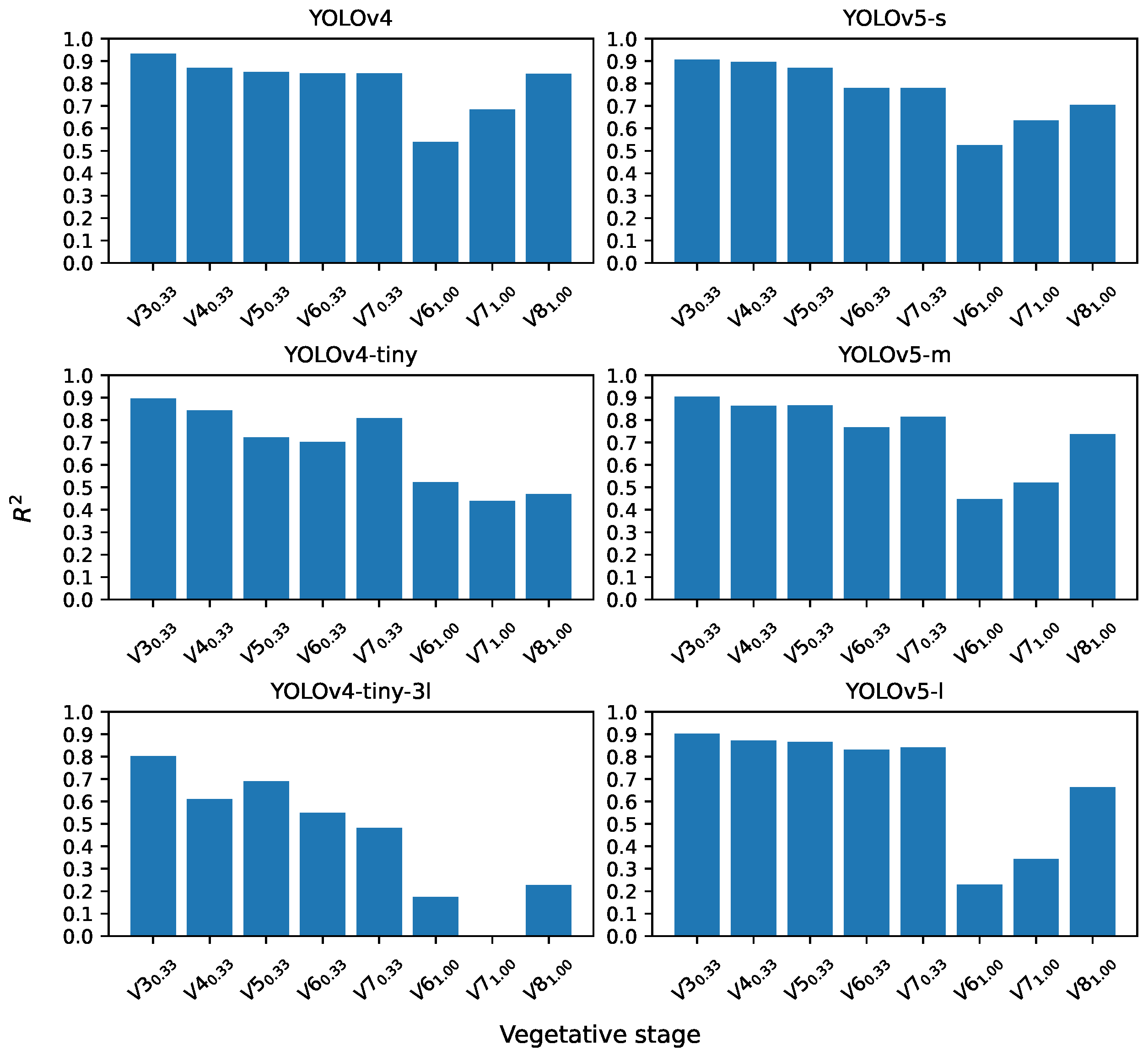
For a better analysis of the data, the models were evaluated for each plant growth stage and their spatial resolution. For the evaluation of the models at stages $V{3}_{0.33}$ and $V{4}_{0.33}$, with the exception of YOLOv4-tiny-3l, the performance results are consistent with the findings reported in the literature. Similar results were found in [21], who reported 10% < rRMSE < 20% for stages V3 and V4 under moderately weedy conditions. In [13] a coefficient $R^2$ = 0.89 is reported for stages V3 and V5, while in [12] $R^2$ = 0.98 is reported for stage V2.

For the YOLOv4-tiny and YOLOv4-tiny-3l models, the results considerably decay from the $V{5}_{0.33}$, stage, which is understandable since they reduce the number of convolutional layers. In addition, the idea that YOLOv4-tiny-3l performs better than YOLOv4-tiny by having one more output was rejected.

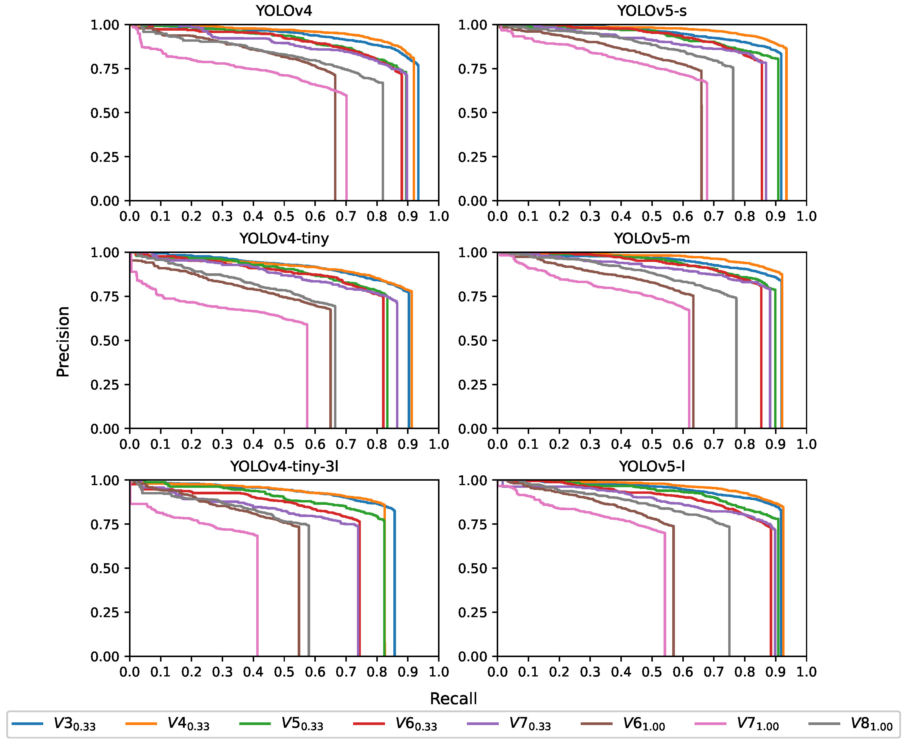
The YOLOv4 models and the YOLOv5 versions evaluated at stages $V{5}_{0.33}$, $V{6}_{0.33}$ and $V{7}_{0.33}$ maintain the results of 70% < Pr < 80% and 85% < Rc < 90%, with the best scores at $V{5}_{0.33}$ followed by $V{7}_{0.33}$. As the rRMSE values for $V{6}_{0.33}$ and $V{7}_{0.33}$ exceed 20%, the results are considered very poor and poor for $V{5}_{0.33}$. These results are consistent with the limitation mentioned by [6], where plants are prone to leaf overlap, which reduces the overall performance of the YOLO architecture evaluated in this work.

A visual inspection of the detections made by each YOLO model helped to understand that FPs at stages lower than V5 with GSD of 0.33 cm/pixel are due to detections made at the edges of the images and in isolated cases due to confusion with weeds. In these cases, the FP count can be lowered by filtering the results with confidence values greater than 0.30. For stages $V{6}_{0.33}$, $V{7}_{0.33}$, $V{6}_{1.00}$ and $V{7}_{1.00}$, the FPs are mostly due to predictions made for unlabeled plants. Although partial labeling is not recommended in tasks addressed with supervised learning, in this case.=, full labeling was extremely complicated due to various errors in the image. Even so, the robustness of the YOLOv5-s model for detecting corn plants under highly complex weed conditions can be seen in Figure 14b.

Although in [20], the effect of spatial resolution on the detection of corn plants was evaluated, obtaining better results with a GSD of 0.3 cm/pixel in stages between V3 and V5, in this work it was observed that, for stages higher than V5, a GSD greater than 0.3 but lower than 1.00 cm/pixel should be considered because the images become difficult to visually interpret for labeling.

Finally, due to the characteristics of the camera mounted on the drone used in this research work, the flight height at which the best results were obtained was 10 m (GSD = 0.33 cm/pixel), which makes large-scale deployment unfeasible due to the limited data acquisition capability. Better cameras that allow for the acquisition of sharper images with plant-level detail at higher flight heights are required for better results when detecting corn plants and to make the application feasible. Another limitation of this study is that a range of GSD was not explored to determine an optimum for the detection of corn plants at vegetative stages above V5.

5. Conclusions

In this research work, a database of aerial images of corn crops with different levels of weed infestation and ground sampling distance was created. The detection and counting of corn plants were evaluated using YOLOv4, YOLOv4-tiny, YOLOv4-tiny-3l, YOLOv5-s, YOLOv5-m and YOLOv5-l architectures. It was shown that YOLOv5 and YOLOv4 architectures are robust in detecting and counting corn plants at stages below V5 in high-resolution images (GSD = 0.33 cm/pixel) even under weed infestation conditions, obtaining Pr results between 77 and 85%, an Rc above 90% and rRMSE between 10 and 20%.

However, in case of stages after V5 with GSD of 1.00 cm/pixel, the results were not favorable, due to the low quality of the images, which did not even allow for the complete labeling of the corn plants. High-resolution images are crucial to improve the results in plant detection; therefore, it is recommended to determine an optimal GSD for the acquisition of aerial images in stages after V5.

The effect of considering different confidence values and IoU thresholds as evaluating detection models was also observed. In this case, YOLOv4 has higher confidence levels than the YOLOv5 versions, although the YOLOv5 versions are more accurate in determining plant location and size. The largest errors in plant counts were obtained in case of the tiny versions of YOLOv4 due to the reduced number of convolutional layers.

Finally, to make plant detection feasible on a larger scale, one direction for future work would be to explore the use of super-resolution architectures coupled to an end-to-end trainable detector, solving the problem of acquiring low-resolution images.

References

1. SIAP. Anuario Estadístico de la Producción Agrícola. 2022. Available online: https://nube.siap.gob.mx/cierreagricola/ (accessed on 3 August 2022).
2. Flores-Cruz, L.A.; García-Salazar, J.A.; Mora-Flores, J.S.; Pérez-Soto, F. Maize production (Zea mays L.) in the state of Puebla: Using spatial equilibrium approach to identify the most competitive producing zones. Agric. Soc. 2014, 11, 223–239. [Google Scholar]
3. Panday, U.S.; Pratihast, A.K.; Aryal, J.; Kayastha, R.B. A Review on Drone-Based Data Solutions for Cereal Crops. Drones 2020, 4, 41. [Google Scholar] [CrossRef]
4. Kitano, B.T.; Mendes, C.C.T.; Geus, A.R.; Oliveira, H.C.; Souza, J.R. Corn Plant Counting Using Deep Learning and UAV Images. IEEE Geosci. Remote Sens. 2019, 1–5. [Google Scholar] [CrossRef]
5. Osco, L.P.; dos Santos de Arruda, M.; Gonçalves, D.N.; Dias, A.; Batistoti, J.; de Souza, M.; Gomes, F.D.G.; Ramos, A.P.M.; de Castro Jorge, L.A.; Liesenberg, V.; et al. A CNN approach to simultaneously count plants and detect plantation-rows from UAV imagery. ISPRS J. Photogramm. Remote Sens. 2021, 174, 1–17. [Google Scholar] [CrossRef]
6. Varela, S.; Dhodda, P.R.; Hsu, W.H.; Prasad, P.V.V.; Assefa, Y.; Peralta, N.R.; Griffin, T.; Sharda, A.; Ferguson, A.; Ciampitti, I.A. Early-Season Stand Count Determination in Corn via Integration of Imagery from Unmanned Aerial Systems (UAS) and Supervised Learning Techniques. Remote Sens. 2018, 10, 343. [Google Scholar] [CrossRef]
7. Messina, G.; Modica, G. Applications of UAV Thermal Imagery in Precision Agriculture: State of the Art and Future Research Outlook. Remote Sens. 2020, 12, 1491. [Google Scholar] [CrossRef]
8. Oh, S.; Chang, A.; Ashapure, A.; Jung, J.; Dube, N.; Maeda, M.; Gonzalez, D.; Landivar, J. Plant Counting of Cotton from UAS Imagery Using Deep Learning-Based Object Detection Framework. Remote Sens. 2020, 12, 2981. [Google Scholar] [CrossRef]
9. Fan, Z.; Lu, J.; Gong, M.; Xie, H.; Goodman, E.D. Automatic Tobacco Plant Detection in UAV Images via Deep Neural Networks. IEEE J. Sel. Top. Appl. Earth Obs. Remote Sens. 2018, 11, 876–887. [Google Scholar] [CrossRef]
10. Valente, J.; Sari, B.; Kooistra, L.; Kramer, H.; Mücher, S. Automated crop plant counting from very high-resolution aerial imagery. Precis. Agric. 2020, 21, 1366–1384. [Google Scholar] [CrossRef]
11. Khaki, S.; Safaei, N.; Pham, H.; Wang, L. WheatNet: A lightweight convolutional neural network for high-throughput image-based wheat head detection and counting. Neurocomputing 2022, 489, 78–89. [Google Scholar] [CrossRef]
12. García-Martínez, H.; Flores-Magdaleno, H.; Khalil-Gardezi, A.; Ascencio-Hernández, R.; Tijerina-Chávez, L.; Vázquez-Peña, M.A.; Mancilla-Villa, O.R. Digital Count of Corn Plants Using Images Taken by Unmanned Aerial Vehicles and Cross Correlation of Templates. Agronomy 2020, 10, 469. [Google Scholar] [CrossRef] [Green Version]
13. Gnädinger, F.; Schmidhalter, U. Digital Counts of Maize Plants by Unmanned Aerial Vehicles (UAVs). Remote Sens. 2017, 9, 544. [Google Scholar] [CrossRef]
14. Shuai, G.; Martinez-Feria, R.A.; Zhang, J.; Li, S.; Price, R.; Basso, B. Capturing Maize Stand Heterogeneity Across Yield-Stability Zones Using Unmanned Aerial Vehicles (UAV). Sensors 2019, 19, 4446. [Google Scholar] [CrossRef] [PubMed]
15. Gómez-Ramos, M.; Ruíz-Castilla, J.; García-Lamont, F. Clasificación de plantas de maíz y maleza: Hacia la mejora de la fertilización en México. Res. Comput. Sci. 2020, 149, 683–697. [Google Scholar]
16. Pang, Y.; Shi, Y.; Gao, S.; Jiang, F.; Veeranampalayam-Sivakumar, A.N.; Thompson, L.; Luck, J.; Liu, C. Improved crop row detection with deep neural network for early-season maize stand count in UAV imagery. Comput. Electron. Agric. 2020, 178, 105766. [Google Scholar] [CrossRef]
17. Liu, H.; Sun, H.; Li, M.; Iida, M. Application of Color Featuring and Deep Learning in Maize Plant Detection. Remote Sens. 2020, 12, 2229. [Google Scholar] [CrossRef]
18. Wang, L.; Xiang, L.; Tang, L.; Jiang, H. A Convolutional Neural Network-Based Method for Corn Stand Counting in the Field. Sensors 2021, 21, 507. [Google Scholar] [CrossRef] [PubMed]
19. Vong, C.N.; Conway, L.S.; Zhou, J.; Kitchen, N.R.; Sudduth, K.A. Early corn stand count of different cropping systems using UAV-imagery and deep learning. Comput. Electron. Agric. 2021, 186, 106214. [Google Scholar] [CrossRef]
20. Velumani, K.; Lopez-Lozano, R.; Madec, S.; Guo, W.; Gillet, J.; Comar, A.; Baret, F. Estimates of Maize Plant Density from UAV RGB Images Using Faster-RCNN Detection Model: Impact of the Spatial Resolution. Plant Phenomics 2021, 2021, 9824843. [Google Scholar] [CrossRef]
21. David, E.; Daubige, G.; Joudelat, F.; Burger, P.; Comar, A.; de Solan, B.; Baret, F. Plant detection and counting from high-resolution RGB images acquired from UAVs: Comparison between deep-learning and handcrafted methods with application to maize, sugar beet, and sunflower. bioRxiv 2022. [Google Scholar] [CrossRef]
22. Brewer, K.; Clulow, A.; Sibanda, M.; Gokool, S.; Naiken, V.; Mabhaudhi, T. Predicting the Chlorophyll Content of Maize over Phenotyping as a Proxy for Crop Health in Smallholder Farming Systems. Remote Sens. 2022, 14, 518. [Google Scholar] [CrossRef]
23. Tzutalin. LabelImg. 2015. Available online: https://github.com/tzutalin/labelImg (accessed on 20 May 2021).
24. Wang, Z.; Wu, Y.; Yang, L.; Thirunavukarasu, A.; Evison, C.; Zhao, Y. Fast Personal Protective Equipment Detection for Real Construction Sites Using Deep Learning Approaches. Sensors 2021, 21, 3478. [Google Scholar] [CrossRef]
25. Lin, T.Y.; Maire, M.; Belongie, S.; Bourdev, L.; Girshick, R.; Hays, J.; Perona, P.; Ramanan, D.; Zitnick, C.L.; Dollár, P. Microsoft COCO: Common Objects in Context. In European Conference on Computer Vision; Springer: Cham, Switzerland, 2014. [Google Scholar] [CrossRef]
26. Voulodimos, A.; Doulamis, N.; Doulamis, A.; Protopapadakis, E. Deep Learning for Computer Vision: A Brief Review. Comput. Intell. Neurosci. 2018, 2018, 7068349. [Google Scholar] [CrossRef]
27. Santos, C.F.G.D.; Papa, J.a.P. Avoiding Overfitting: A Survey on Regularization Methods for Convolutional Neural Networks. ACM Comput. Surv. 2022, 54, 1–25. [Google Scholar] [CrossRef]
28. Sozzi, M.; Cantalamessa, S.; Cogato, A.; Kayad, A.; Marinello, F. Automatic Bunch Detection in White Grape Varieties Using YOLOv3, YOLOv4, and YOLOv5 Deep Learning Algorithms. Agronomy 2022, 12, 319. [Google Scholar] [CrossRef]
29. Wenkel, S.; Alhazmi, K.; Liiv, T.; Alrshoud, S.; Simon, M. Confidence Score: The Forgotten Dimension of Object Detection Performance Evaluation. Sensors 2021, 21, 4350. [Google Scholar] [CrossRef]
30. Bochkovskiy, A.; Wang, C.Y.; Liao, H.Y.M. YOLOv4: Optimal Speed and Accuracy of Object Detection. arXiv 2020, arXiv:2004.10934. [Google Scholar] [CrossRef]
31. Jocher, G.; Chaurasia, A.; Stoken, A.; Borovec, J.; NanoCode012; Kwon, Y.; Xie, T.; Fang, J.; imyhxy; Michael, K.; et al. Ultralytics/yolov5: V6.1—TensorRT, TensorFlow Edge TPU and OpenVINO Export and Inference. 2022. Available online: https://github.com/ultralytics/yolov5 (accessed on 5 March 2022).
32. Redmon, J.; Divvala, S.; Girshick, R.; Farhadi, A. You Only Look Once: Unified, Real-Time Object Detection. In Proceedings of the 2016 IEEE Conference on Computer Vision and Pattern Recognition (CVPR), Las Vegas, NV, USA, 27–30 June 2016; pp. 779–788. [Google Scholar] [CrossRef]
33. Redmon, J.; Farhadi, A. YOLOv3: An Incremental Improvement. arXiv 2018, arXiv:1804.02767. [Google Scholar]
34. Nepal, U.; Eslamiat, H. Comparing YOLOv3, YOLOv4 and YOLOv5 for Autonomous Landing Spot Detection in Faulty UAVs. Sensors 2022, 22, 464. [Google Scholar] [CrossRef] [PubMed]
35. Padilla, R.; Passos, W.L.; Dias, T.L.B.; Netto, S.L.; da Silva, E.A.B. A Comparative Analysis of Object Detection Metrics with a Companion Open-Source Toolkit. Electronics 2021, 10, 279. [Google Scholar] [CrossRef]
36. Everingham, M.; Eslami, S.; Van Gool, L.; Williams, C.K.; Winn, J.; Zisserman, A. The PASCAL Visual Object Classes Challenge: A Retrospective. Int. J. Comput. Vis. 2015, 111, 98–136. [Google Scholar] [CrossRef]
37. Yang, B.; Gao, Z.; Gao, Y.; Zhu, Y. Rapid Detection and Counting of Wheat Ears in the Field Using YOLOv4 with Attention Module. Agronomy 2021, 11, 1202. [Google Scholar] [CrossRef]
Figure 1. Location and distribution of experimental sites.
Remotesensing 14 04892 g001
Figure 2. Manually labeled image samples. (a,b) correspond to Irrigación with corn at stage V 4 0.33 , (c) to San Juan A2 with corn at stage V 8 1.00 , (d) to Xerona with corn at stage V 6 1.00 , (e) to Ranchito X13 with corn at stage V 7 1.00 and (f) to Irrigación with corn at stage V 6 0.33 .
Remotesensing 14 04892 g002
Figure 3. Distribution of the database according to vegetative stage and GSD.
Remotesensing 14 04892 g003
Figure 4. Distribution of the labels according to the area in p i x e l s 2 for an image size of 416 × 416 pixels.
Remotesensing 14 04892 g004
Figure 5. Diagram of the YOLOv4 architecture with an input image of 416 × 416 pixels and 3 channels.
Remotesensing 14 04892 g005
Figure 6. Diagram of the YOLOv4-tiny-3l architecture with an input image of 416 × 416 pixels and 3 channels.
Remotesensing 14 04892 g006
Figure 7. Diagram of the YOLOv5-l (V6.0/6.1) architecture with an input image of 416 × 416 pixels and 3 channels.
Remotesensing 14 04892 g007
Figure 8. [email protected] calculated for the test set during training of the CNN algorithms with a confidence of 0.25.
Remotesensing 14 04892 g008
Figure 9. F1-Score vs. Confidence curves at IoU thresholds 0.25, 0.50 and 0.75 for each trained model.
Remotesensing 14 04892 g009
Figure 10. YOLOv5-l architecture detections for a confidence of 0.3 with an IoU threshold of 0.5 (a) and 0.25 (b). The blue boxes represent the ground truth label, green ones TP and red ones FP.
Remotesensing 14 04892 g010
Figure 11. Recall vs. Precision curves by vegetative stage and spatial resolution.
Remotesensing 14 04892 g011
Figure 12. rRMSE obtained for each model by vegetative stage and spatial resolution.
Remotesensing 14 04892 g012
Figure 13. R 2 determined for each vegetative stage considering detections with a confidence level greater than 0.30 and IoU of 0.25.
Remotesensing 14 04892 g013
Figure 14. Visualization of manually labeled images (blue box), TP (green box) and FP (red box). Detection of vegetative stage (a) V 3 with YOLOv4, (b) V 7 1.00 with YOLOv5-s, (c) V 8 1.00 with YOLOv5-s and (d) V 6 1.00 with YOLOv5-s.
Remotesensing 14 04892 g014