

Spatiotemporal Prediction of Monthly Sea Subsurface Temperature Fields Using a 3D U-Net-Based Model

Abstract

1. Introduction
2. Related Works
3. Data
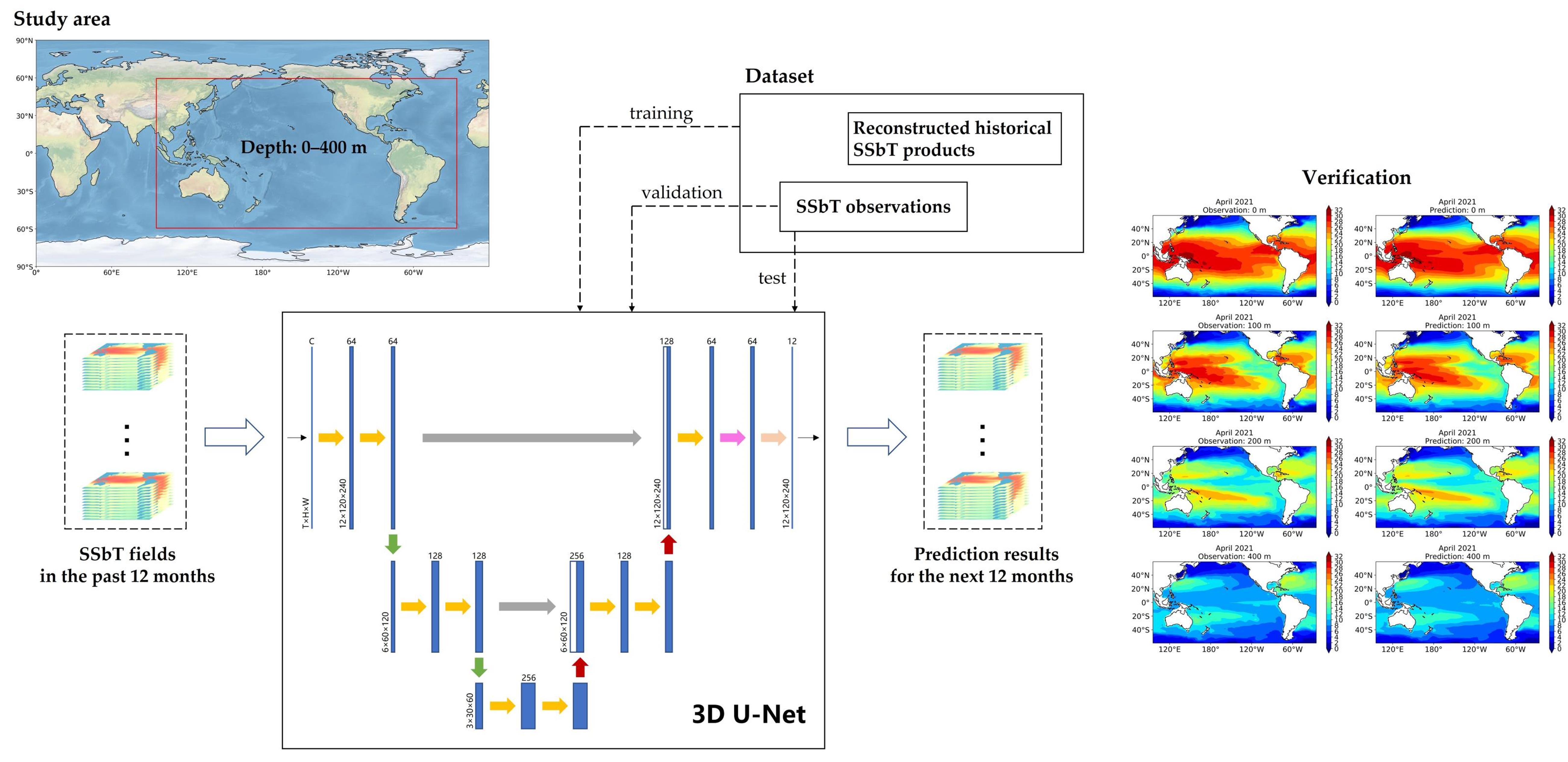
4. Method
5. Experiments
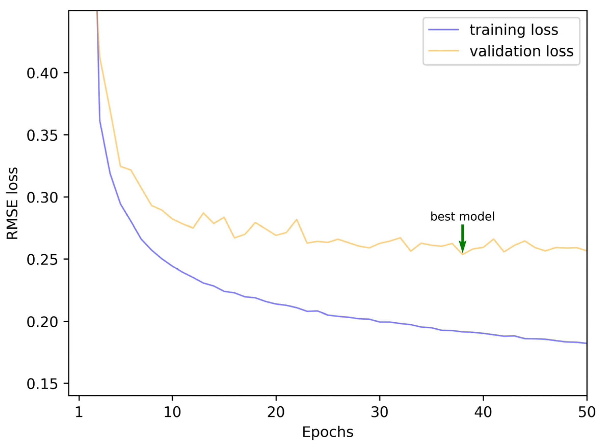
5.1. Experimental Settings
5.2. Evaluation Metrics
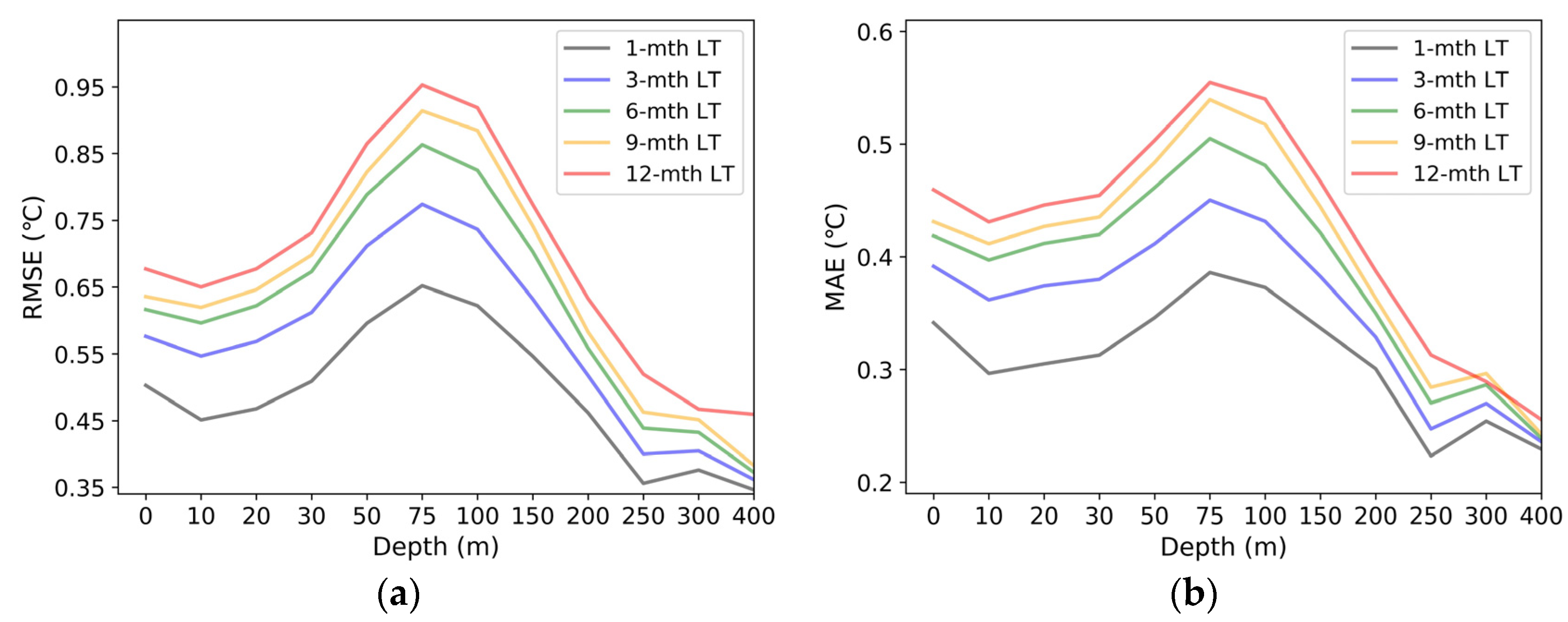
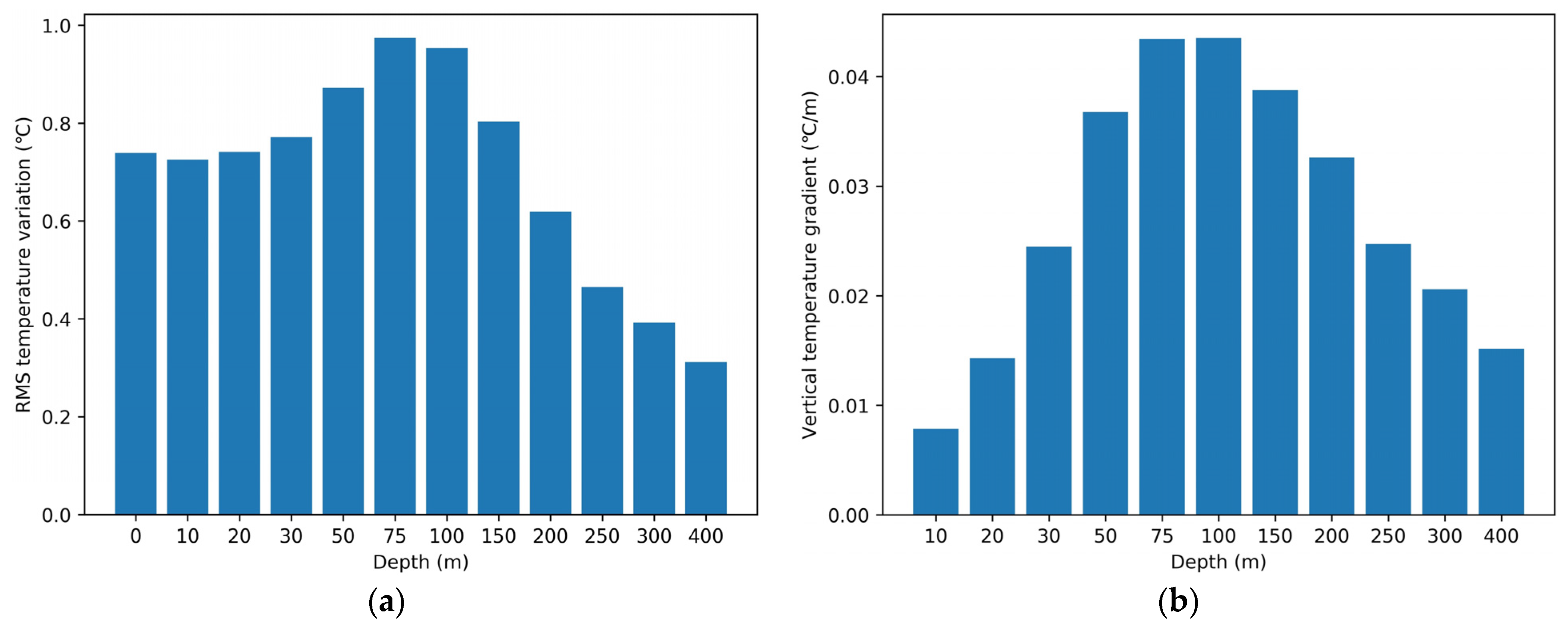
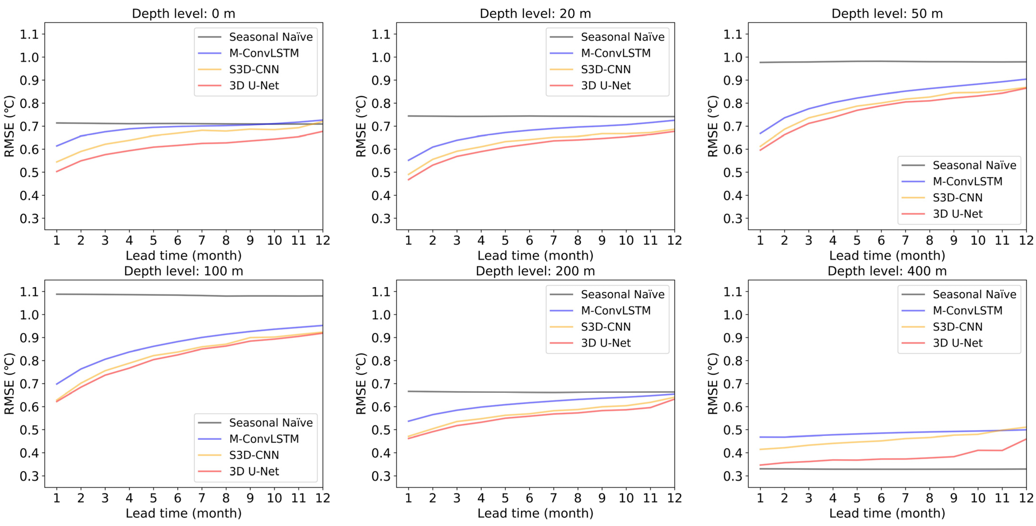
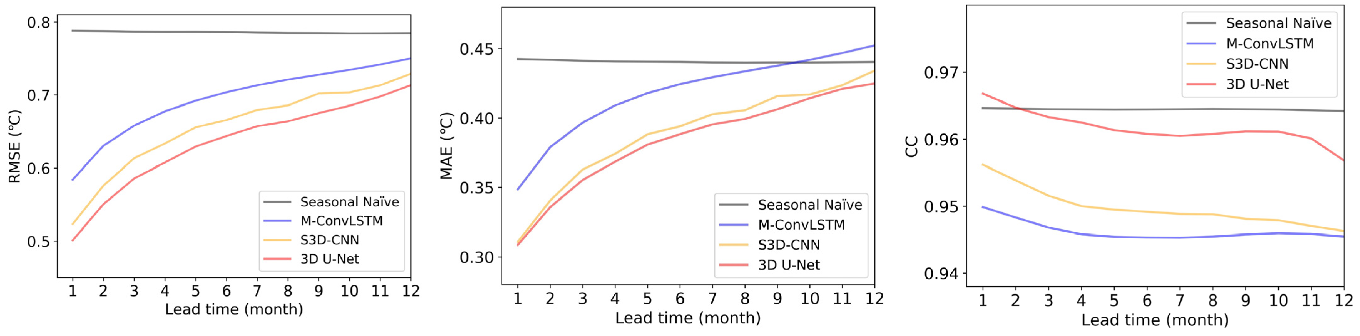
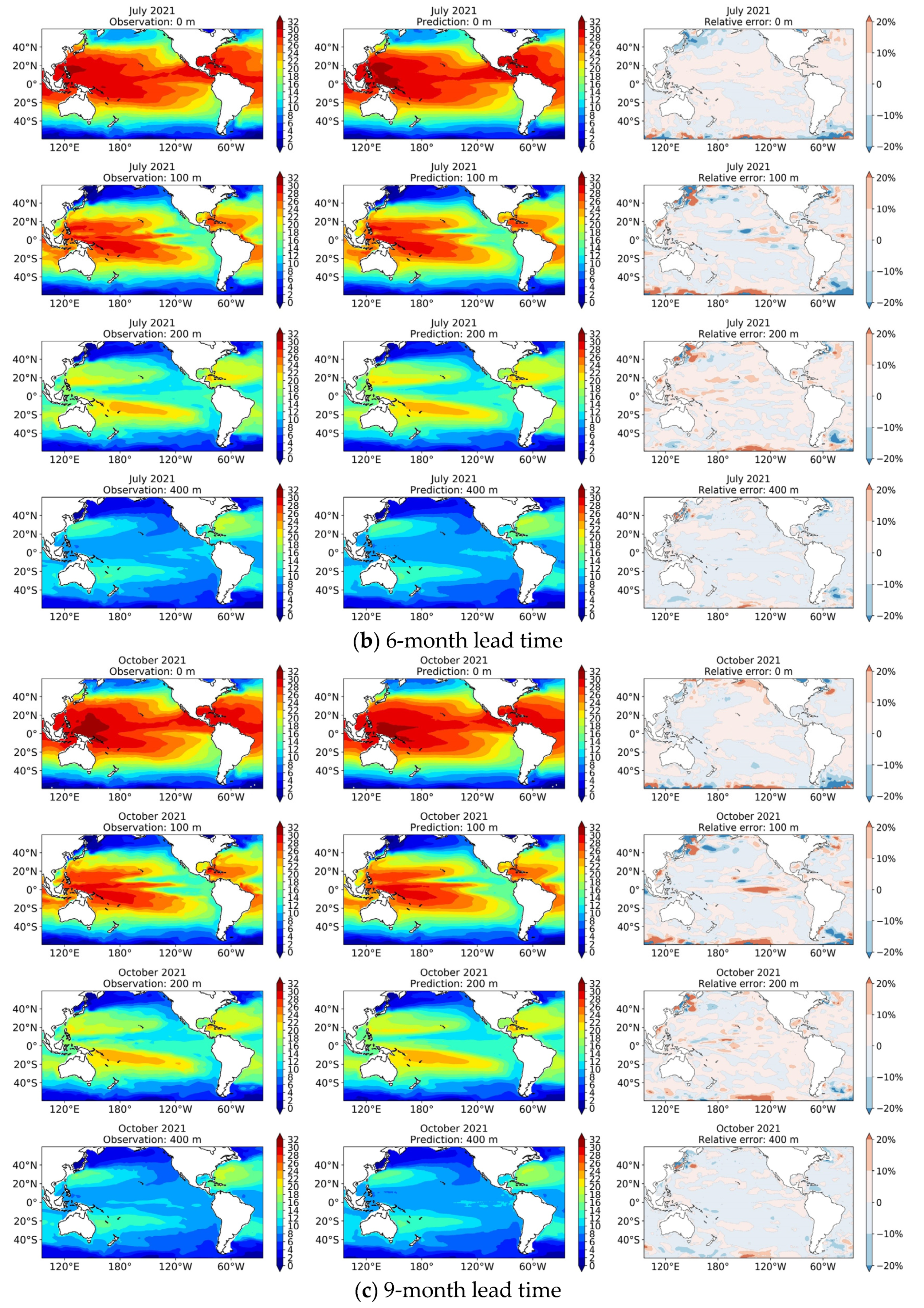
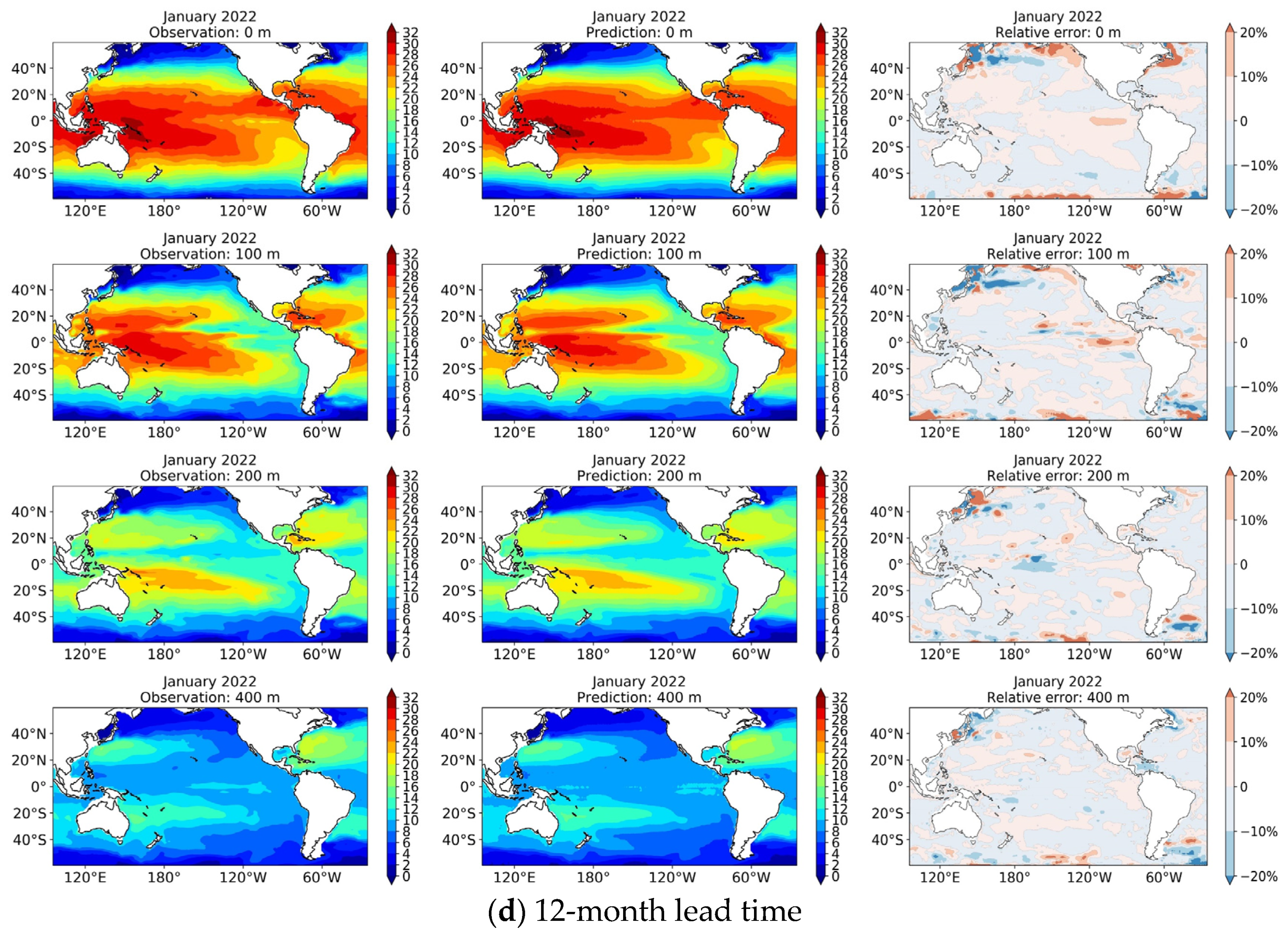
5.3. Results
6. Conclusions
Author Contributions
Funding
Data Availability Statement
Acknowledgments
Conflicts of Interest
References
- Wentz, F.J.; Gentemann, C.; Smith, D.; Chelton, D. Satellite measurements of sea surface temperature through clouds. Science 2000, 288, 847–850. [Google Scholar] [CrossRef] [PubMed]
- Yao, S.L.; Luo, J.J.; Huang, G.; Wang, P. Distinct global warming rates tied to multiple ocean surface temperature changes. Nat. Clim. Change 2017, 7, 486–491. [Google Scholar] [CrossRef]
- Kao, H.Y.; Yu, J.Y. Contrasting eastern-Pacific and central-Pacific types of ENSO. J. Clim. 2009, 22, 615–632. [Google Scholar] [CrossRef]
- Anderson, B.T. On the joint role of subtropical atmospheric variability and equatorial subsurface heat content anomalies in initiating the onset of ENSO events. J. Clim. 2007, 20, 1593–1599. [Google Scholar] [CrossRef]
- Cione, J.J.; Uhlhorn, E.W. Sea surface temperature variability in hurricanes: Implications with respect to intensity change. Mon. Weather. Rev. 2003, 131, 1783–1796. [Google Scholar] [CrossRef]
- Belkin, I.M. Rapid warming of large marine ecosystems. Prog. Oceanogr. 2009, 81, 207–213. [Google Scholar] [CrossRef]
- Gou, Y.; Zhang, T.; Liu, J.; Wei, L.; Cui, J.H. DeepOcean: A general deep learning framework for spatio-temporal ocean sensing data prediction. IEEE Access 2020, 8, 79192–79202. [Google Scholar] [CrossRef]
- Klemas, V. Fisheries applications of remote sensing: An overview. Fish. Res. 2013, 148, 124–136. [Google Scholar] [CrossRef]
- Barnston, A.G.; Glantz, M.H.; He, Y. Predictive skill of statistical and dynamical climate models in SST forecasts during the 1997–98 El Niño episode and the 1998 La Niña onset. Bull. Am. Meteorol. Soc. 1999, 80, 217–244. [Google Scholar] [CrossRef]
- Stockdale, T.N.; Balmaseda, M.A.; Vidard, A. Tropical Atlantic SST prediction with coupled ocean–atmosphere GCMs. J. Clim. 2006, 19, 6047–6061. [Google Scholar] [CrossRef]
- Johnson, S.J.; Stockdale, T.N.; Ferranti, L.; Balmaseda, M.A.; Molteni, F.; Magnusson, L.; Monge-Sanz, B.M. SEAS5: The new ECMWF seasonal forecast system. Geosci. Model Dev. 2019, 12, 1087–1117. [Google Scholar] [CrossRef]
- Kondrashov, D.; Kravtsov, S.; Robertson, A.W.; Ghil, M. A hierarchy of data-based ENSO models. J. Clim. 2005, 18, 4425–4444. [Google Scholar] [CrossRef]
- Shirvani, A.; Nazemosadat, S.M.J.; Kahya, E. Analyses of the Persian Gulf sea surface temperature: Prediction and detection of climate change signals. Arab. J. Geosci. 2015, 8, 2121–2130. [Google Scholar] [CrossRef]
- Lins, I.D.; Araujo, M.; das Chagas Moura, M.; Silva, M.A.; Droguett, E.L. Prediction of sea surface temperature in the tropical Atlantic by support vector machines. Comput. Stat. Data Anal. 2013, 61, 187–198. [Google Scholar] [CrossRef]
- Corchado, J.M.; Fyfe, C. Unsupervised neural method for temperature forecasting. Artif. Intell. Eng. 1999, 13, 351–357. [Google Scholar] [CrossRef]
- Wei, L.; Guan, L.; Qu, L. Prediction of sea surface temperature in the South China Sea by artificial neural networks. IEEE Geosci. Remote Sens. Lett. 2019, 17, 558–562. [Google Scholar] [CrossRef]
- Zhang, Q.; Wang, H.; Dong, J.; Zhong, G.; Sun, X. Prediction of sea surface temperature using long short-term memory. IEEE Geosci. Remote Sens. Lett. 2017, 14, 1745–1749. [Google Scholar] [CrossRef]
- Ham, Y.G.; Kim, J.H.; Luo, J.J. Deep learning for multi-year ENSO forecasts. Nature 2019, 573, 568–572. [Google Scholar] [CrossRef]
- Haghbin, M.; Sharafati, A.; Motta, D.; Al-Ansari, N.; Noghani, M.H.M. Applications of soft computing models for predicting sea surface temperature: A comprehensive review and assessment. Prog. Earth Planet. Sci. 2021, 8, 1–19. [Google Scholar] [CrossRef]
- Zhang, Z.; Pan, X.; Jiang, T.; Sui, B.; Liu, C.; Sun, W. Monthly and quarterly sea surface temperature prediction based on gated recurrent unit neural network. J. Mar. Sci. Eng. 2020, 8, 249. [Google Scholar] [CrossRef]
- Yang, Y.; Dong, J.; Sun, X.; Lima, E.; Mu, Q.; Wang, X. A CFCC-LSTM model for sea surface temperature prediction. IEEE Geosci. Remote Sens. Lett. 2017, 15, 207–211. [Google Scholar] [CrossRef]
- Shi, X.; Chen, Z.; Wang, H.; Yeung, D.Y.; Wong, W.K.; Woo, W.-C. Convolutional LSTM network: A machine learning approach for precipitation nowcasting. Adv. Neural Inf. Process. Syst. 2015, 28, 802–810. [Google Scholar]
- Xiao, C.; Chen, N.; Hu, C.; Wang, K.; Xu, Z.; Cai, Y.; Gong, J. A spatiotemporal deep learning model for sea surface temperature field prediction using time-series satellite data. Environ. Model. Softw. 2019, 120, 104502. [Google Scholar] [CrossRef]
- Gupta, M.; Kodamana, H.; Sandeep, S. Prediction of ENSO beyond spring predictability barrier using deep convolutional LSTM networks. IEEE Geosci. Remote Sens. Lett. 2020, 19, 1501205. [Google Scholar] [CrossRef]
- Zhang, K.; Geng, X.; Yan, X.H. Prediction of 3-D ocean temperature by multilayer convolutional LSTM. IEEE Geosci. Remote Sens. Lett. 2020, 17, 1303–1307. [Google Scholar] [CrossRef]
- Wu, X.; Yan, X.H.; Jo, Y.H.; Liu, W.T. Estimation of subsurface temperature anomaly in the North Atlantic using a self-organizing map neural network. J. Atmos. Ocean. Technol. 2012, 29, 1675–1688. [Google Scholar] [CrossRef]
- Cheng, L.; Zhu, J. Benefits of CMIP5 multimodel ensemble in reconstructing historical ocean subsurface temperature variations. J. Clim. 2016, 29, 5393–5416. [Google Scholar] [CrossRef]
- Liu, J.; Zhang, T.; Han, G.; Gou, Y. TD-LSTM: Temporal dependence-based LSTM networks for marine temperature prediction. Sensors 2018, 18, 3797. [Google Scholar] [CrossRef]
- Patil, K.R.; Iiyama, M. Deep Neural Networks to Predict Sub-surface Ocean Temperatures from Satellite-Derived Surface Ocean Parameters. In Soft Computing for Problem Solving; Springer: Singapore, 2021; pp. 423–434. [Google Scholar]
- Zuo, X.; Zhou, X.; Guo, D.; Li, S.; Liu, S.; Xu, C. Ocean temperature prediction based on stereo spatial and temporal 4-D convolution model. IEEE Geosci. Remote Sens. Lett. 2021, 19, 1–5. [Google Scholar] [CrossRef]
- Ishii, M.; Kimoto, M.; Sakamoto, K.; Iwasaki, S. Subsurface Temperature and Salinity Analyses; Research Data Archive at the National Center for Atmospheric Research. Accessed 4 June 2022; Computational and Information Systems Laboratory: Boulder, CO, USA, 2005. [Google Scholar] [CrossRef]
- Reynolds, R.W.; Rayner, N.A.; Smith, T.M.; Stokes, D.C.; Wang, W. An improved in situ and satellite SST analysis for climate. J. Clim. 2002, 15, 1609–1625. [Google Scholar] [CrossRef]
- Behringer, D.W.; Ji, M.; Leetmaa, A. An improved coupled model for ENSO prediction and implications for ocean initialization. Part I: The ocean data assimilation system. Mon. Weather. Rev. 1998, 126, 1013–1021. [Google Scholar] [CrossRef]
- Yang, K.; Cai, W.; Huang, G.; Wang, G.; Ng, B.; Li, S. Oceanic processes in ocean temperature products key to a realistic presentation of positive Indian Ocean Dipole nonlinearity. Geophys. Res. Lett. 2020, 47, e2020GL089396. [Google Scholar] [CrossRef]
- Tang, Y.; Duan, A. Using deep learning to predict the East Asian summer monsoon. Environ. Res. Lett. 2021, 16, 124006. [Google Scholar] [CrossRef]
- Çiçek, Ö.; Abdulkadir, A.; Lienkamp, S.S.; Brox, T.; Ronneberger, O. U-net: Learning dense volumetric segmentation from sparse annotation. In Proceedings of the International Conference on Medical Image Computing and Computer-Assisted Intervention, Athens, Greece, 17–21 October 2016; Springer: Cham, Switzerland, 2016; pp. 424–432. [Google Scholar]
- Ioffe, S.; Szegedy, C. Batch normalization: Accelerating deep network training by reducing internal covariate shift. In Proceedings of the International Conference on Machine Learning, Lille, France, 7–9 July 2015; pp. 448–456. [Google Scholar]
- Tran, D.; Bourdev, L.; Fergus, R.; Torresani, L.; Paluri, M. Learning spatiotemporal features with 3d convolutional networks. In Proceedings of the IEEE International Conference on Computer Vision, Santiago, Chile, 7–13 December 2015; pp. 4489–4497. [Google Scholar]
- Abadi, M.; Agarwal, A.; Barham, P.; Brevdo, E.; Chen, Z.; Citro, C.; Zheng, X. Tensorflow: Large-Scale Machine Learning on Heterogeneous Distributed Systems. arXiv 2016, arXiv:1603.04467. [Google Scholar]
- Doney, S.; Yeager, S.; Danabasoglu, G.; Large, W.; McWilliams, J. Modeling Global Oceanic Interannual Variability (1958–1997): Simulation Design and Model-Data Evaluation; Tech. Note NCAR/TN-452+ STR; National Center for Atmospheric Research: Boulder, CO, USA, 2003. [Google Scholar]
- Zhang, Y.; Li, K.; Li, K.; Wang, L.; Zhong, B.; Fu, Y. Image super-resolution using very deep residual channel attention networks. In Proceedings of the European Conference on Computer Vision (ECCV), Munich, Germany, 8–14 September 2018; pp. 286–301. [Google Scholar]


| Subset | Product | Period | Number of Sequences |
|---|---|---|---|
| Training | IAP | January 1956–December 2007 | 1623 |
| RDA | January 1945–December 2007 | ||
| OISST V2 and GODAS | January 1982–December 2007 | ||
| Validation | OISST V2 and GODAS | January 2008–December 2012 | 60 |
| Test | OISST V2 and GODAS | January 2013–May 2022 | 102 |
| Dataset | RMSE | MAE | CC |
|---|---|---|---|
| Observation data | 0.6857 | 0.4227 | 0.9506 |
| Reconstructed data + observation data | 0.6343 | 0.3832 | 0.9616 |
| Depth | North Temperate | North Subtropics | Tropics | South Subtropics | South Temperate |
|---|---|---|---|---|---|
| 0 | 0.7323 | 0.6200 | 0.5363 | 0.5468 | 0.5876 |
| 20 | 0.7194 | 0.5811 | 0.6003 | 0.4648 | 0.5256 |
| 50 | 0.7754 | 0.6334 | 0.9259 | 0.4568 | 0.5182 |
| 100 | 0.6494 | 0.6109 | 1.0686 | 0.4424 | 0.5179 |
| 200 | 0.5163 | 0.4657 | 0.6488 | 0.4376 | 0.4540 |
| 400 | 0.4180 | 0.4123 | 0.3924 | 0.3407 | 0.3147 |
| Region | RMSE | MAE | CC |
|---|---|---|---|
| North temperate | 0.6391 | 0.3330 | 0.9177 |
| North subtropics | 0.5565 | 0.3718 | 0.9935 |
| Tropics | 0.7345 | 0.4454 | 0.9960 |
| South subtropics | 0.4492 | 0.3130 | 0.9955 |
| South temperate | 0.4893 | 0.3499 | 0.9081 |
Publisher’s Note: MDPI stays neutral with regard to jurisdictional claims in published maps and institutional affiliations. |
© 2022 by the authors. Licensee MDPI, Basel, Switzerland. This article is an open access article distributed under the terms and conditions of the Creative Commons Attribution (CC BY) license (https://creativecommons.org/licenses/by/4.0/).
Share and Cite
Sun, N.; Zhou, Z.; Li, Q.; Zhou, X. Spatiotemporal Prediction of Monthly Sea Subsurface Temperature Fields Using a 3D U-Net-Based Model. Remote Sens. 2022, 14, 4890. https://doi.org/10.3390/rs14194890
Sun N, Zhou Z, Li Q, Zhou X. Spatiotemporal Prediction of Monthly Sea Subsurface Temperature Fields Using a 3D U-Net-Based Model. Remote Sensing. 2022; 14(19):4890. https://doi.org/10.3390/rs14194890
Chicago/Turabian StyleSun, Nengli, Zeming Zhou, Qian Li, and Xuan Zhou. 2022. "Spatiotemporal Prediction of Monthly Sea Subsurface Temperature Fields Using a 3D U-Net-Based Model" Remote Sensing 14, no. 19: 4890. https://doi.org/10.3390/rs14194890
APA StyleSun, N., Zhou, Z., Li, Q., & Zhou, X. (2022). Spatiotemporal Prediction of Monthly Sea Subsurface Temperature Fields Using a 3D U-Net-Based Model. Remote Sensing, 14(19), 4890. https://doi.org/10.3390/rs14194890