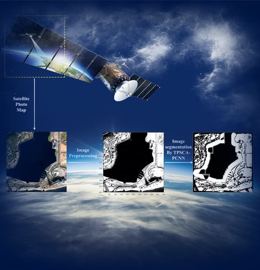
Optimization of Remote Sensing Image Segmentation by a Customized Parallel Sine Cosine Algorithm Based on the Taguchi Method

Abstract

Affected by solar radiation, atmospheric windows, radiation aberrations, and other air and sky environmental factors, remote sensing images usually contain a large amount of noise and suffer from problems such as non-uniform image feature density. These problems bring great difficulties to the segmentation of high-precision remote sensing image. To improve the segmentation effect of remote sensing images, this study adopted an improved metaheuristic algorithm to optimize the parameter settings of pulse-coupled neural networks (PCNNs). Using the Taguchi method, the optimal parallelism scheme of the algorithm was effectively tailored for a specific target problem. The blindness in the design of the algorithm parallel structure was effectively avoided. The superiority of the customized parallel SCA based on the Taguchi method (TPSCA) was demonstrated in tests with different types of benchmark functions. In this study, simulations were performed using IKONOS, GeoEye-1, and WorldView-2 satellite remote sensing images. The results showed that the accuracy of the proposed remote sensing image segmentation model was significantly improved.

1. Introduction

With the development of remote sensing technology, the number of remote sensing images is growing exponentially. How to effectively utilize the huge amount of remote sensing images has become a challenging task. Accurate segmentation of remote sensing images facilitates better analyses of acquired images [1]. The accuracy and spatial resolution of remote sensing images are increasing, which makes it possible to distinguish different kinds of observation objects. However, at the same time, it also puts higher requirements on segmentation techniques. In addition, RGB remote sensing images have been used on large scales, and the rich color space further increases the difficulty of image segmentation.

According to the different segmentation mechanisms, remote sensing image segmentation can be divided into four categories: spectral-based image segmentation [2], spatial-based image segmentation [3], hybrid-technology-based image segmentation [4], and semantic-based image segmentation [5]. Spectral-based remote sensing image segmentation is mainly based on analyzing individual pixels of images, including segmentation based on thresholding [6] and segmentation based on feature space clustering [7]. Spatial-based remote sensing image segmentation includes edge-based image segmentation [8], region-based image segmentation [9], and graph-based image segmentation [10]. Image segmentation based on hybrid technology combines the above methods. Unlike the first three types of segmentation methods that focus on extracting similar regions, semantic-based image segmentation achieves segmentation by pairing each pixel in a remote sensing image with the label of its corresponding object. However, it is possible to overemphasize certain unnecessary details in the image.

The existing threshold-based image segmentation technology has been extended to multi-level thresholds to assist in the segmentation of multi-channel images [11]. However, image segmentation based on multi-level threshold has the disadvantage of high time complexity. With the increase in pixel channels, the efficiency of the traditional method using exhaustive searches in color remote sensing image segmentation has decreased dramatically. The metaheuristic algorithm with excellent optimization ability provides an effective solution to this problem. The sine cosine algorithm (SCA) [12] is a population-based metaheuristic algorithm that solves optimization problems through swarm intelligence. The search individual moves in the solution space according to the trajectory determined by the sine or cosine function. The algorithm has few control parameters and simple structure, and has good performance in many practical optimization problems [13,14,15].

In recent years, neural networks (NNs) have often been used in image processing, such as U-Net [16] and deep convolutional neural networks [17], which have achieved good results in image segmentation. However, this kind of model will be affected by the gradient; they are prone to gradient explosion and are time-consuming in the training process. It is known that the spatial complexity determines the number of parameters of the model. Additionally, a high model complexity can easily lead to overfitting problems in image processing. U-Net extracts features by stacking conventional convolution and lacks the ability to model long-term dependencies autonomously; thus, U-Net has a high computational complexity. The spatial complexity of a convolutional neural network is $\mathrm{Space}~\mathrm{O}\left({\displaystyle \sum }_{l=1}^D{K}_l^2·C_{l-1}·C_l+{\displaystyle \sum }_{l=1}^D{M}^2·C_l\right)$, where $K$ is the convolutional kernel size, $C$ is the number of channels, and $D$ is the number of neural network layers. As the first third-generation neural network, pulse-coupled neural networks (PCNNs) [3] successfully avoid the adverse effect of gradient and reduce the spatial complexity of the model using pulse coding. In this model, a variety of image processing procedures, such as image segmentation [18] and edge detection [19], are realized through synchronous pulse distribution and global coupling. The key to the performance of PCNN lies in the selection of initial parameters [20]. It is difficult to guarantee the validity of the model by subjectively selecting parameters. This study used the modified SCA to optimize the parameters of the PCNN to improve the segmentation effect of remote sensing images.

To improve the segmentation of the model, scholars have found that using bio-inspired or nature-inspired methods to solve the proposed problem is an effective improvement. Sarkar et al. proposed a decomposition-based multi-objective evolutionary algorithm with DE optimization algorithm to propose an image segmentation technique that relies on entropy and multi-level thresholding [21]. Zhang et al. introduced a quantum particle swarm optimization algorithm to propose a real-time image segmentation method for distinguishing the target image from the navigation image [22]. In this study, we used the sine cosine algorithm compared with some traditional metaheuristic algorithms, which has the characteristics of fewer parameters, fast convergence, high exploration accuracy, and good stability; therefore, we used the improved SCA to optimize the parameters of the pulse-coupled neural network to improve the segmentation effect of remote sensing images.

Parallel processing can significantly enhance the optimization ability of metaheuristic algorithms [23,24]. The search population is divided into several subpopulations, where adequate communication between subpopulations is developed to prevent the algorithm from falling into local optima [25]. The parallel scheme needs to be designed according to the nature of the target problem. This paper presents a customized parallel SCA based on the Taguchi method (TPSCA). According to Taguchi’s method [26], the suitable parallel structure of the algorithm for the target problem can be obtained through a small number of experiments, which realizes the automation of parallel scheme design to a certain extent.

The main contributions of this paper are as follows:

• A parallel SCA (PSCA) with three different communication strategies is proposed to solve the unimodal, multimodal, and complex problems;
• Using Taguchi’s method to obtain a customized parallel SCA scheme (TPSCA);
• A high-performance remote sensing image segmentation model is constructed by combining TPSCA with PCNN.

The structure of this paper is as follows: the second part introduces studies related to the technologies involved; the third part describes the proposed customized parallel SCA based on the Taguchi method; the fourth part uses benchmark functions to test TPSCA and analyze the experimental results; the fifth part introduces the combination of TPSCA and PCNN; the sixth part is the simulation experiment and analysis of remote sensing image segmentation; the seventh part is the conclusion and future work.

2. Related Works

2.1. Sine Cosine Algorithm (SCA)

The SCA is a population intelligence optimization algorithm proposed by Mirjalili in 2016, and its search process is mainly influenced by the sine and cosine function. SCA uses initial random solutions, then asks them to fluctuate outward or toward the best solution based on sine and cosine functions. The search process of the SCA can be divided into exploration and exploitation, and the position update formulas for both phases are shown in Equation (1):

$$\left\{\begin{array}{c}{X}_i^{t+1}=X_i^t+r_1\times \sin \left(r_2\right)\times \left|r_3{P}_i^t-X_i^t\right|, r_4\ge 0.5\\ X_i^{t+1}=X_i^t+r_1\times \cos \left(r_2\right)\times \left|r_3{P}_i^t-X_i^t\right|, r_4<0.5\end{array}\right.$$

(1)

where $t$ is the current number of iterations, $X_i^t$ is the position of the $i$-th dimension in the $t$-th iteration, $P_i^t$ is the position of the objective individual in the i-th dimension, and $r_1/r_2/r_3$ are random numbers. $\left|·\right|$ is the absolute value. When $r_1>1$, the SCA uses a larger search space for global exploration; when $r_1\le 1$, SCA uses a smaller search space for local exploitation. $r_1$ is updated according to Equation (2):

$$r_1=a-t\frac{a}{T}$$

(2)

where $a>0,a\in C$, and $T$ is the maximum number of iterations.

The SCA tends to converge prematurely, and it can easily fall into local optima when optimizing complex problems. Some scholars have improved the process of the SCA. To enhance the global search capability of the algorithm, Belazzoug et al. [27] added a crossover operation between random individuals and optimal individuals. Qu et al. [28] added the neighborhood search to the existing search method of the SCA to better balance the algorithm’s local exploitation and global exploration. Even though optimization performance can be improved by improving the algorithmic process, it increases the time complexity of the SCA. Some scholars have started to improve parameters of the SCA. Ji et al. [29] proposed an adaptive modification to the parameter $r_1$ of the SCA to make the algorithm transition smoother between global exploration and local exploitation. Moreover, algorithm hybridization is a common method to improve the metaheuristic algorithm; Chegini et al. [30] hybridized the SCA with a particle swarm optimization algorithm (PSO), and Dey et al. [31] hybridized the SCA with a whale optimization algorithm (WOA). Both studies improved the optimization ability of the algorithm to some extent.

2.2. Taguchi Method

The Taguchi method is a low-cost and highly efficient engineering method widely used in industrial production [32,33,34]. Taguchi emphasizes robust design to improve product quality while reducing random errors [35,36]. Orthogonal tables and signal-to-noise ratios are important bases and tools of Taguchi method, respectively. The orthogonal table is used to establish the test plan, and the signal-to-noise ratio (SNR) is used to evaluate the quality merit. Adjusting the level of controllable factors weakens the influence of noise on quality characteristics, and improves the interference resistance of the customized design. In this study, we added the Taguchi method into the design of the metaheuristics algorithm: $N_t$ is the number of repeat experiments, and the quality characteristic is the objective function value of the algorithm ($fitness$). A larger signal-to-noise ratio means better results, and the optimization task can be categorized as solving the minimization problem. Therefore, when $fitness\ge 0$, we used Equation (3) to calculate the smaller-the-better signal-to-noise ratio and the larger-the-better signal-to-noise ratio as shown in Equation (4) when $fitness<0$.

$$\mathrm{SNR}=-10\log (\frac{1}{N_t}{\displaystyle \sum }_{i=1}^{N_t}fitnes{s}^2)$$

(3)

$$\mathrm{SNR}=-10\log (\frac{1}{N_t}{\displaystyle \sum }_{i=1}^{N_t}\frac{1}{fitnes{s}^2})$$

(4)

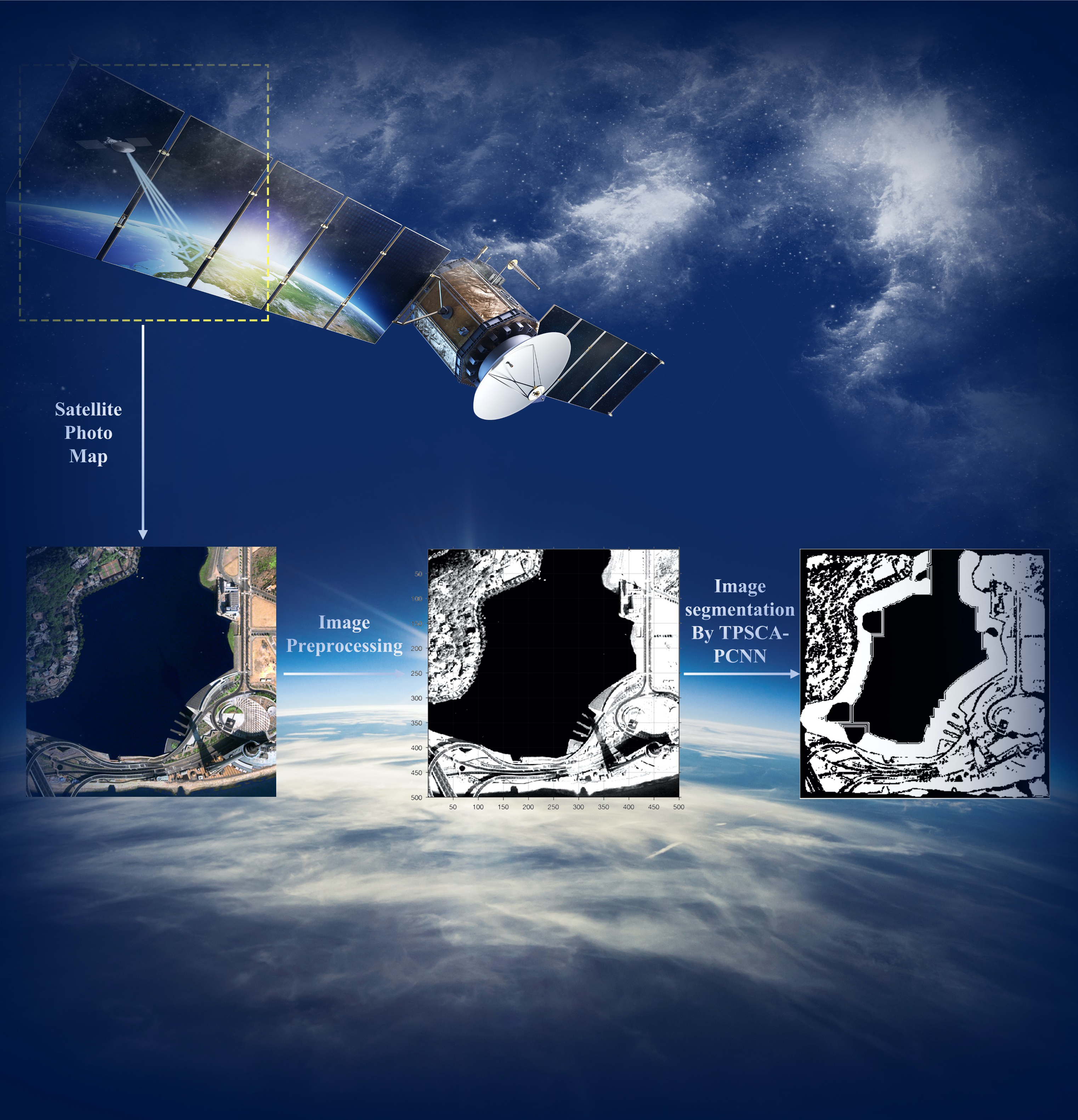
2.3. Pulse-Coupled Neural Networks (PCNNs)

PCNNs are artificial neural networks that imitate the characteristics of biological vision. They can use the currently activated neuron to trigger similar neurons around it; thus, they are especially suitable for solving image processing problems, such as image denoising, image enhancement, image fusion, image segmentation, and edge detection [37,38,39,40,41]. PCNN-based image segmentation methods have achieved many practical applications, such as agricultural crop recognition [42], medical image segmentation [43], and remote sensing satellite detection [44]. Different from deep learning methods, PCNNs do not require extensive training for extracting image features [45], and can thus solve image segmentation problems in unknown domains.

PCNNs consist of three parts, and include the input layer, connection layer, and pulse generator. The basic working principle of the neuron is shown in Figure 1, and the neuron model can be represented by Equations (5)–(9).

$$F_{i,j}\left[n\right]=e^{-{\alpha }_F}{F}_{i,j}\left[n-1\right]+V_F{{\displaystyle \sum }}_{k,l}{M}_{i,j,k,l}{Y}_{i,j}\left[n-1\right]+S_{i,j}$$

(5)

$$L_{i,j}\left[n\right]=e^{-{\alpha }_L}{L}_{i,j}\left[n-1\right]+V_L{{\displaystyle \sum }}_{k,l}{W}_{i,j,k,l}{Y}_{i,j}\left[n-1\right]$$

(6)

$$U_{i,j}\left[n\right]=F_{i,j}\left[n\right]\left(1+\beta L_{i,j}\left[n\right]\right)$$

(7)

$$Y_{i,j}\left[n\right]=\left\{\begin{array}{c}1,U_{i,j}\left[n\right]>T_{i,j}\left[n\right]\\ 0,otherwise\end{array}\right.$$

(8)

$$T_{i,j}\left[n\right]=e^{-{\alpha }_T}{T}_{i,j}\left[n-1\right]+V_T{Y}_{i,j}\left[n\right]$$

(9)

where $F_{i,j}\left[n\right]$ is the feedback input term of the neuron, $L_{i,j}\left[n\right]$ is the link term, $U_{i,j}\left[n\right]$ represents the internal activity of the neuron, $S_{i,j}$ represents the gray value of pixel point $\left(i,j\right)$, $T_{i,j}\left[n\right]$ is the dynamic threshold, and $Y_{i,j} \left[n\right]$ represents the binary output of the model. β denotes the link factor, and ${\alpha }_F$, ${\alpha }_L$, and ${\alpha }_T$ are decay rates. $V_F$, $V_L$, and $V_T$ are amplification factors. $M_{\left(i,j,k,l\right)}$ and $W_{\left(i,j,k,l\right)}$ are the synaptic connection weight matrix, reflecting the influence of peripheral neurons on central neurons.

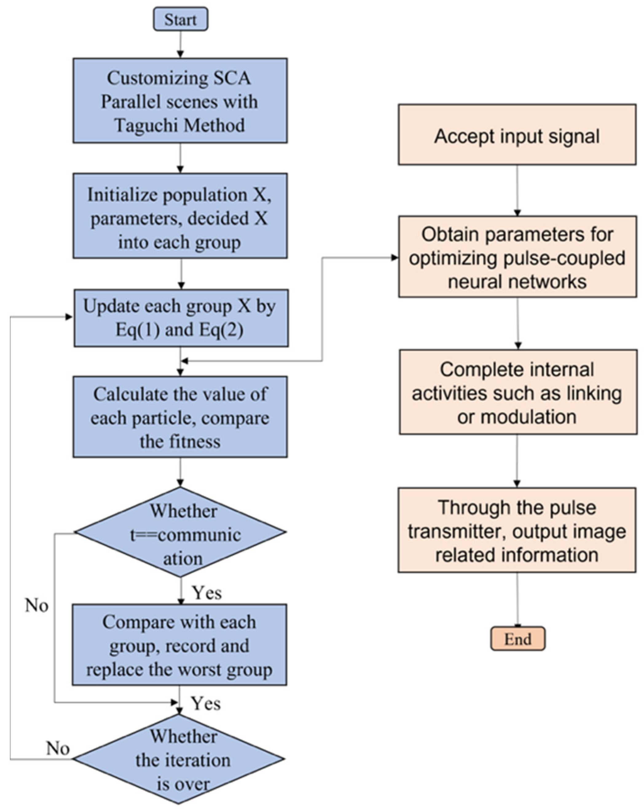
3. Customized Parallel SCA (TPSCA) Based on the Taguchi Method

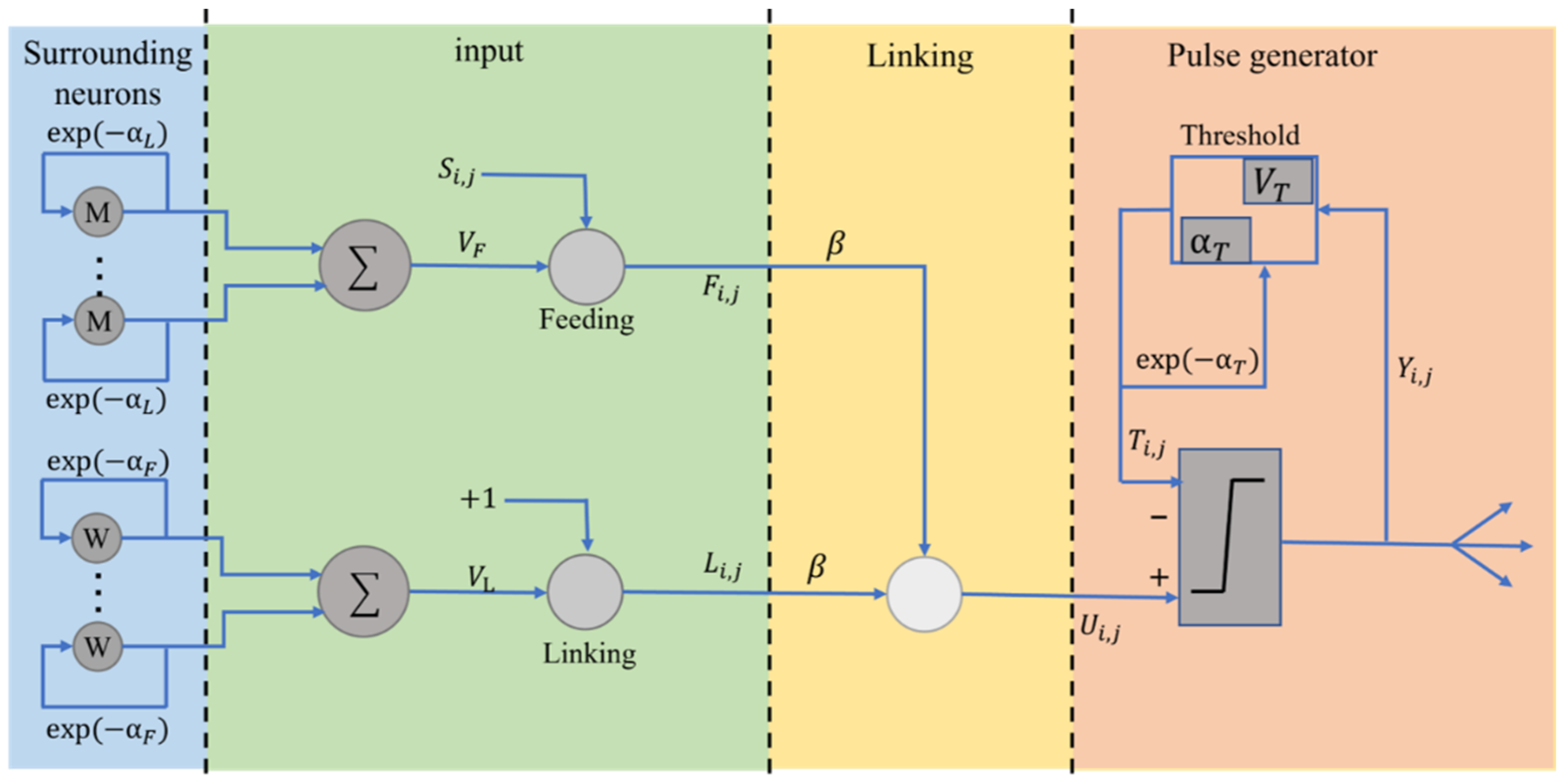
3.1. Parallel Sine Cosine Algorithm (PSCA)

To further improve the optimization performance of the SCA, we used the parallel method to improve it, which generally includes the following operations:

• Dividing population: dividing the whole population into several subpopulations;
• Communication: exchange between subpopulations every $t$ generation during the iterative process;
• Integration: update the population based on the results of the communication.

The parallel method can effectively enhance the diversity of populations and avoid stagnation of the local optimal which can be combined with distributed computing techniques to improve the algorithm operation efficiency as well. Considering the different types of objective functions in practical problems, a simplex parallel method cannot solve all problems. Therefore, we propose three parallel communication strategies for unimodal, multimodal, and complex problems: Strategy 1: Parallel SCA based on the optimal value replacement (PSCA-Best). The execution flow is shown in Figure 2. Firstly, the population is divided into $g$ groups, each subgroup containing $i$ individuals, and the $i$-th individual of group g is $x_i^g$. Each subgroup is searched independently and communicated after several iterations. The current global optimum is used to replace the worst value of each subgroup, fully using the leading role of the global optimal solution. Strategy 1 can effectively enhance the local exploitation ability of the algorithm and improve the search efficiency in the unimodal problem.

Strategy 2: Parallel SCA based on optimal mean replacement (PSCA- Mean). The execution flow is shown in Figure 3. There are several extrema of the multimodal problem and consider jump out of the local optimum. In Strategy 1, the search method is dominated by the global optimum, and it will easily fall into the local optimum when solving the multimodal problem. Therefore, the second parallel communication strategy, PSCA-Mean, is proposed for optimizing the multimodal problem, which uses the optimal average value to replace the worst value of each group without relying too much on the current global optimum. Thus, Strategy 2 can make full use of the search individuals of each group and enhance the global search capability of the algorithm.

Strategy 3: Hybrid parallel SCA (PSCA-Hybrid). When optimizing complex problems, relying solely on Strategy 1 or Strategy 2 often does not guarantee a comprehensive and effective search. If an optimization problem of an unknown type is encountered, blindly determining the communication strategy cannot ensure the optimization effect. Therefore, the third parallel communication strategy is proposed to consider the advantages of Strategy 1 and Strategy 2, and use them interchangeably. In this study, we used 23 benchmark functions to test the performance of the algorithm; these included the unimodal problem, multimodal problem, and complex problem, as shown in

Table 1. Unimodal functions.

Function	Dim	${\mathit{f}}_{\mathit{m}\mathit{i}\mathit{n}}$
$f_1\left(x\right)={\displaystyle \sum }_{i=1}^n{x}_i^2$	20	0
$f_2\left(x\right)={\displaystyle \sum }_{i=1}^n\left|x_i\right|+{\displaystyle \prod }_{i=1}^n\left|x_i\right|$	20	0
$f_3\left(x\right)={\displaystyle \sum }_{i=1}^n{\left({\displaystyle \sum }_{j=1}^i{x}_j\right)}^2$	20	0
$f_4\left(x\right)=\max \left\{\left|x_i\right|,1\le i\le n\right\}$	20	0
$f_5\left(x\right)={\displaystyle \sum }_{i=1}^{n-1}{\displaystyle [}100{\left(x_{i+1}-x_i^2\right)}^2+{\left(x_i-1\right)}^2{\displaystyle ]}$	20	0
$f_6\left(x\right)={\displaystyle \sum }_{i=1}^n{\left(\left[x_i+0.5\right]\right)}^2$	20	0
$f_7\left(x\right)={\displaystyle \sum }_{i=1}^{n}i{x}_i^4+random\left[0,1\right]$	20	0

,

Table 2. Multimodal functions.

Function	Dim	${\mathit{f}}_{\mathit{m}\mathit{i}\mathit{n}}$
$f_8\left(x\right)={\displaystyle \sum }_{i=1}^n-x_i\sin \left(\sqrt{\left|x_i\right|}\right)$	20	−418.9829 × 5
$f_9\left(x\right)={\displaystyle \sum }_{i=1}^n\left[x_i^2-10\cos \left(2\pi x_i\right)+10\right]$	20	0
$f_{10}\left(x\right)=-20\exp \left(-0.2\sqrt{\frac{1}{n}{\displaystyle \sum }_{i=1}^n{x}_i^2}\right)-\exp \left(\frac{1}{n}{\displaystyle \sum }_{i=1}^n\cos \left(2\pi x_i\right)\right)+20+e$	20	0
$f_{11}\left(x\right)=\frac{1}{4000}{\displaystyle \sum }_{i=1}^n{x}_i^2-{\displaystyle \prod }_{i=1}^n\cos \left(\frac{x_i}{\sqrt{i}}\right)+1$	20	0
$f_{12}\left(x\right)=\frac{\pi }{n}\left\{10\sin \left(\pi y_1\right)+{\displaystyle \sum }_{i=1}^{n-1}{(y_i-1)}^2\left[1+10{\sin }^2\left(\pi y_{i+1}\right)\right]+\left(y_n-1\right)\right\}+{\displaystyle \sum }_{i=1}^{n}u\left(x_i,10,100,4\right)$	20	0
$f_{13}\left(x\right)=0.1{\sin }^2\left(3\pi x_i\right)+{\displaystyle \sum }_{i=1}^n{\left(x_i-1\right)}^2\left[1+{\sin }^2\left(3\pi x_i+1\right)\right]+\left(x_n-1\right)\left[1+{\sin }^2\left(2\pi x_n\right)\right]\}$	20	0

and

Table 3. Complex functions.

Function	Dim	${\mathit{f}}_{\mathit{m}\mathit{i}\mathit{n}}$
$f_{14}\left(x\right)={\left(\frac{1}{500}+{\displaystyle \sum }_{i=1}^n\left(\frac{1}{random\left[1,25\right]+bs\left(i\right)}\right)\right)}^{-1}$	2	0
$f_{15}\left(x\right)={\displaystyle \sum }_{i=1}^n\left(ak-{\left(\frac{\left(x\left(1\right)\left(b{k}^2+x\left(2\right)bk\right)\right)}{b{k}^2+x\left(3\right)bk+x\left(4\right)}\right)}^2\right)$	4	0.0003
$f_{16}\left(x\right)=4\left(x{\left(1\right)}^2\right)-2.1\left(x{\left(1\right)}^4\right)+\frac{1}{3}\left(x{\left(1\right)}^6\right)+x\left(1\right)x\left(2\right)-4\left(x{\left(2\right)}^2\right)+4 \left(x{\left(2\right)}^4\right)$	2	−1.0316
$f_{17}\left(x\right)={\left(x\left(2\right)-\frac{\left(x{\left(1\right)}^{2}5.1\right)}{\left(4\left({\pi }^2\right)\right)}+\frac{5}{\pi x\left(1\right)-6}\right)}^2+10\left(1-\frac{1}{8\pi }\right)\cos \left(x\left(1\right)+10\right)$	2	0.398
$f_{18}\left(x\right)={\left(1+x\left(1\right)+x\left(2\right)+1\right)}^2\left(19-14x\left(1\right)+3\left(x{\left(1\right)}^2\right)-14x\left(2\right)+6x\left(1\right)x\left(2\right)+3x{\left(2\right)}^2\right))\left(30+\left(2x\left(1\right)\right)\right)$	2	3
$f_{19}\left(x\right)=f_{19}\left(x\right)-cH\left(i\right)\ast \exp \left(-\left({\displaystyle \sum }_{i=1}^{n}aH\left(i\right)\ast \left({\left(x-pH\left(i\right)\right)}^2\right)\right)\right)$	3	−3.86
$f_{20}\left(x\right)=f_{20}\left(x\right)-cH\left(i\right)\ast \exp \left(-\left({\displaystyle \sum }_{i=1}^{n}aH\left(i\right)\ast \left({\left(x-pH\left(i\right)\right)}^2\right)\right)\right)$	6	−3.32
$f_{21} \left(x\right)=f_{21}\left(x\right)-\left(\left(x-aSH\left(i\right)\right)\ast \left(x-aSH\left(i\right)\right)+cSH\left(i\right)\right)^\left(-1\right),i=1:5$	4	−10.1532
$f_{22}\left(x\right)=f_{22}\left(x\right)-\left(\left(x-aSH\left(i\right)\right)\ast \left(x-aSH\left(i\right)\right)+cSH\left(i\right)\right)^\left(-1\right),i=1:7$	4	−10.4028
$f_{23}\left(x\right)=f_{23}\left(x\right)-\left(\left(x-aSH\left(i\right)\right)\ast \left(x-aSH\left(i\right)\right)+cSH\left(i\right)\right)^\left(-1\right), i=1:10$	4	−10.5363

.

To compare the effectiveness of the three SCA parallel communication strategies, six typical functions are selected for testing, including two unimodal functions (F1 and F2), two multimodal functions (F8 and F12), and two complex functions (F16 and F23). Each procedure was run 20 times independently. The best value, average value, and standard deviation obtained by the algorithm were recorded and are shown in

Table 4. The comparison test of the SCA, PSCA-Best, PSCA-Mean, and PSCA-Hybrid.

Function	Algorithm	Best Fitness	Mean	STD
F1	SCA	$1.83\times {10}^{-18}$	$7.51\times {10}^{-11}$	$1.83\times {10}^{-10}$
	PSCA-Best	$\mathbf{1.27}\mathbf{\times }{\mathbf{10}}^{\mathbf{-}\mathbf{21}}$	$\mathbf{3.92}\mathbf{\times }{\mathbf{10}}^{\mathbf{-}\mathbf{17}}$	$\mathbf{9.43}\mathbf{\times }{\mathbf{10}}^{\mathbf{-}\mathbf{17}}$
	PSCA-Mean	$1.4\times {10}^{-20}$	$6.31\times {10}^{-15}$	$1.51\times {10}^{-14}$
	PSCA-Hybrid	$1.63\times {10}^{-21}$	$9.36\times {10}^{-16}$	$1.99\times {10}^{-15}$
F2	SCA	$1.83\times {10}^{-15}$	$1.42\times {10}^{-11}$	$3.14\times {10}^{-11}$
	PSCA-Best	$\mathbf{6.21}\mathbf{\times }{\mathbf{10}}^{\mathbf{-}\mathbf{17}}$	$\mathbf{8.8}\mathbf{\times }{\mathbf{10}}^{\mathbf{-}\mathbf{13}}$	$\mathbf{1.37}\mathbf{\times }{\mathbf{10}}^{\mathbf{-}\mathbf{12}}$
	PSCA-Mean	$7.6\times {10}^{-12}$	$4.92\times {10}^{-11}$	$5.13\times {10}^{-11}$
	PSCA-Hybrid	$1.08\times {10}^{-15}$	$2.19\times {10}^{-12}$	$3.45\times {10}^{-12}$
F8	SCA	$-2.26\times {10}^3$	$-2.05\times {10}^3$	$1.13\times {10}^2$
	PSCA-Best	$-2.21\times {10}^3$	$-2.08\times {10}^3$	$1.02\times {10}^2$
	PSCA-Mean	$\mathbf{-}\mathbf{2.34}\mathbf{\times }{\mathbf{10}}^{\mathbf{3}}$	$\mathbf{-}\mathbf{2.23}\mathbf{\times }{\mathbf{10}}^{\mathbf{3}}$	$\mathbf{1.05}\mathbf{\times }{\mathbf{10}}^{\mathbf{2}}$
	PSCA-Hybrid	$-2.23\times {10}^3$	$-2.11\times {10}^3$	$6.94\times {10}^1$
F12	SCA	$7.19\times {10}^{-2}$	$1.23\times {10}^{-1}$	$3.81\times {10}^{-2}$
	PSCA-Best	$8.63\times {10}^{-2}$	$1.45\times {10}^{-1}$	$3.27\times {10}^{-2}$
	PSCA-Mean	$\mathbf{5.42}\mathbf{\times }{\mathbf{10}}^{\mathbf{-}\mathbf{2}}$	$\mathbf{7.37}\mathbf{\times }{\mathbf{10}}^{\mathbf{-}\mathbf{2}}$	$\mathbf{2.48}\mathbf{\times }{\mathbf{10}}^{\mathbf{-}\mathbf{2}}$
	PSCA-Hybrid	$6.41\times {10}^{-2}$	$1.15\times {10}^{-1}$	$4.36\times {10}^{-2}$
F21	SCA	$-4.68$	$-2.86$	$1.56$
	PSCA-Best	$-4.55$	$-3.49$	$8.93$
	PSCA-Mean	$-3.50$	$-2.56$	$1.04$
	PSCA-Hybrid	$\mathbf{-}\mathbf{5.10}$	$\mathbf{-}\mathbf{4.59}$	$\mathbf{5.59}\mathbf{\times }{\mathbf{10}}^{\mathbf{-}\mathbf{1}}$
F22	SCA	$-3.38$	$-3.80$	$4.19\times {10}^{-1}$
	PSCA-Best	$-4.33$	$-3.10$	$7.93\times {10}^{-1}$
	PSCA-Mean	$-4.11$	$-3.25$	$7.67\times {10}^{-1}$
	PSCA-Hybrid	$\mathbf{-}\mathbf{7.48}$	$\mathbf{-}\mathbf{5.05}$	$\mathbf{1.46}$

. The bold numbers represents the best value for each indicator in the table. It can be seen that PSCA-Best is the strongest in solving unimodal problems. This is due to the dominant role of the PSCA-Best strategy to maximize the optimal individual, which reflects the excellent local development capability. When solving multimodal functions, the optimization ability of PSCA-Mean is best, which can effectively jump out of the local optimum to perform a more comprehensive search. PSCA-Hybrid shows a more stable advantage when solving complex functions.

The bold numbers represent the best value for each indicator in Table 4. PSCA-Best performed well in solving unimodal problems, due to the leading role of the maximized optimal individual and reflects the outstanding local exploitation ability. When solving multimodal functions, the optimization ability of PSCA-Mean was best, which could effectively jump out of the local optimum to perform a more comprehensive search. PSCA-Hybrid showed a more stable advantage when solving complex functions.

To further visualize the optimization performance of PSCA, we will present the position of the algorithm in the solution space, the search trajectory, the average fitness, and the convergence curve, which are shown in Figure 4. The first column (a) shows the distribution of solutions in the 2D solution space. The second column (b) shows the search trajectory, which is the change curve of the first dimension of the solution. The third column (c) is the curve of the average fitness value of all individuals. The fourth column (d) shows the convergence curve of the algorithm. In Figure 4a, the red circle is the optimal position in the solution space, and the black circles represent the historical positions. The black circles are randomly distributed in the solution space and gradually approach the optimal red circle as the iteration proceeds. From the one-dimensional search trajectory in Figure 4b, the early search trajectory occupies the entire search space, indicating that the algorithm designed in this paper would have excellent global search capability. In Figure 4c, the average fitness value fluctuates significantly at the beginning stage and then converges to a constant value, which indicates that the algorithm has the fast convergence at the early stage and accurate confluence at the later stage. Figure 4d shows the convergence curves of each algorithm, the three communication strategies have achieved the best results in the corresponding optimization problems.

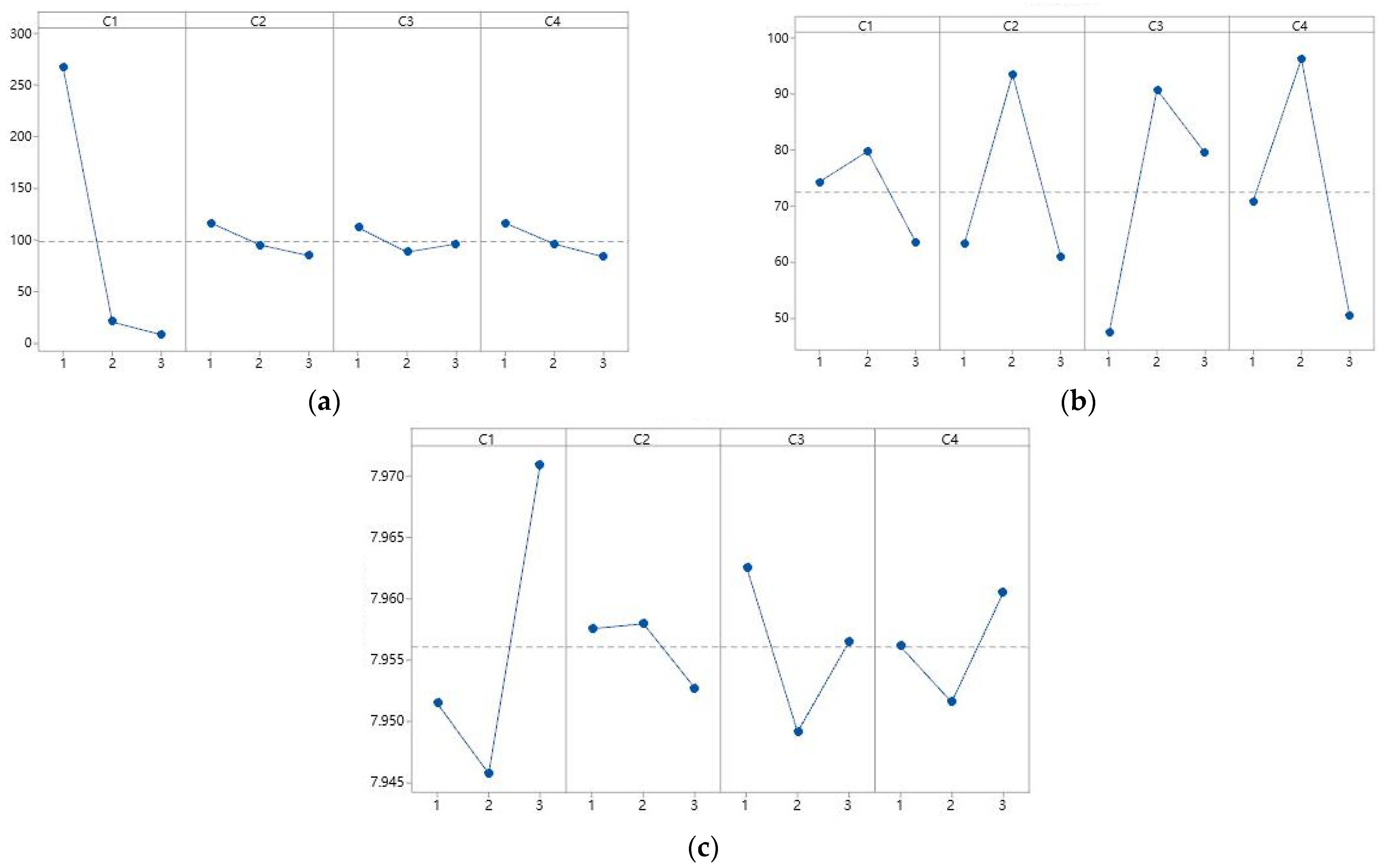
3.2. Custom SCA Parallel Scheme (TPSCA)

Although many novel parallel schemes for metaheuristic algorithms already exist [46], the type of target problem (unimodal/ multimodal/complex) needs to be predicted in order to select some pre-designed parallel scheme, and a suitable parallel structure cannot be configured on site according to the nature of the problem to be solved. Parallel processing can significantly improve the optimization of algorithms without increasing the time complexity. However, the design of parallel structures should not be one-size-fits-all, only one specific parallel scheme suitable for the problem [47]. The key design factors to be considered in the parallel structure are population size $\left(N\right)$, the number of iterations $\left(Miter\right)$, number of groups $\left(G\right)$, communication frequency $\left(\lambda \right)$, and communication strategy $\left(S\right)$. In this study, Taguchi’s method was added into the design of parallel schemes, hoping to automate and customize the design of parallel algorithms using fewer experimental tests to configure a suitable parallel structure for the problem. In the design of TPSCA, four important factors of PSCA were customized. To ensure the fairness of comparison, we set the first factor, $C1$, as (population size N $\times$ number of iterations) $\left(N\times Miter\right)$, the second factor, $C2$, as the number of groups $G$, the third factor, $C3$, as the frequency of communication $\lambda$ (communicate once every λ iterations), and the fourth factor, $C4$, as the communication strategy $S \left(PSCA-Best/ PSCA-Mean/ PSCA-Hybrid\right)$. Each factor had three levels, and the parameter level table is shown in

Table 5. Parameter level table.

Level	$\mathit{N}\times \mathit{M}\mathit{i}\mathit{t}\mathit{e}\mathit{r}$	$\mathit{G}$	$\mathit{\lambda }$	$\mathit{S}$
Level 1	$16\times 800$	2	30	PSCA-Best
Level 2	$32\times 400$	4	50	PSCA-Mean
Level 3	$64\times 200$	8	60	PSCA-Hybrid

. If the full-parameter design method is used, $3^4=81$ trials are required to obtain the best solution, but the Taguchi method only requires 9 experiments to obtain the best-customized solution.

Table 6. Taguchi orthogonal table.

Experiment Group	Considered Factors
	$\mathit{N}\times \mathit{M}\mathit{i}\mathit{t}\mathit{e}\mathit{r}$	$\mathit{G}$	$\mathit{\lambda }$	$\mathit{S}$
1	1	1	1	1
2	2	1	3	2
3	3	1	2	3
4	1	2	2	1
5	2	2	1	3
6	3	2	3	2
7	1	3	1	3
8	2	3	3	1
9	3	3	2	2

shows the orthogonal table $L_9\left(3^4\right)$ for the parallel solution selection trials. As shown in Figure 5, the orthogonal results were analyzed using Equation (3) or Equation (4) to draw the main effects of the signal-to-noise ratio for solving the three types of problems, where the x-axis represents the three levels of each of the four factors, and the y-axis represents the mean value of the signal-to-noise ratio. One function for each unimodal, multimodal, and complex problems was chosen to customize the parallel scheme for them. We can see the different factor levels to influence the optimization effect of the parallel scheme. The highest mean signal-to-noise ratio factor level was selected to obtain the best optimization effect.

With the 23 benchmark tests, we can determine the best scheme of TPSCA in solving the unimodal problem as $\left\{N\ast Miter\left(16\ast 800\right),G\left(2\right),\lambda \left(30\right),S\left(PSCA-Best\right)\right\}$, the best parallel scheme for multimodal problem as $\left\{N\ast Miter\left(32\ast 400\right),G\left(4\right),\lambda \left(50\right),S\left(PSCA-Mean/ PSCA-Hybrid\right)\right\}$, and the best parallel scheme for solving complex problems as $\left\{N\ast Miter\left(64\ast 200\right),G\left(4\right),\lambda \left(30\right),S\left(PSCA-Hybrid\right)\right\}$. The customized results of the communication strategy are consistent with the experimental results in Section 3.1, indicating the effectiveness of the automatic customization of the Taguchi method.

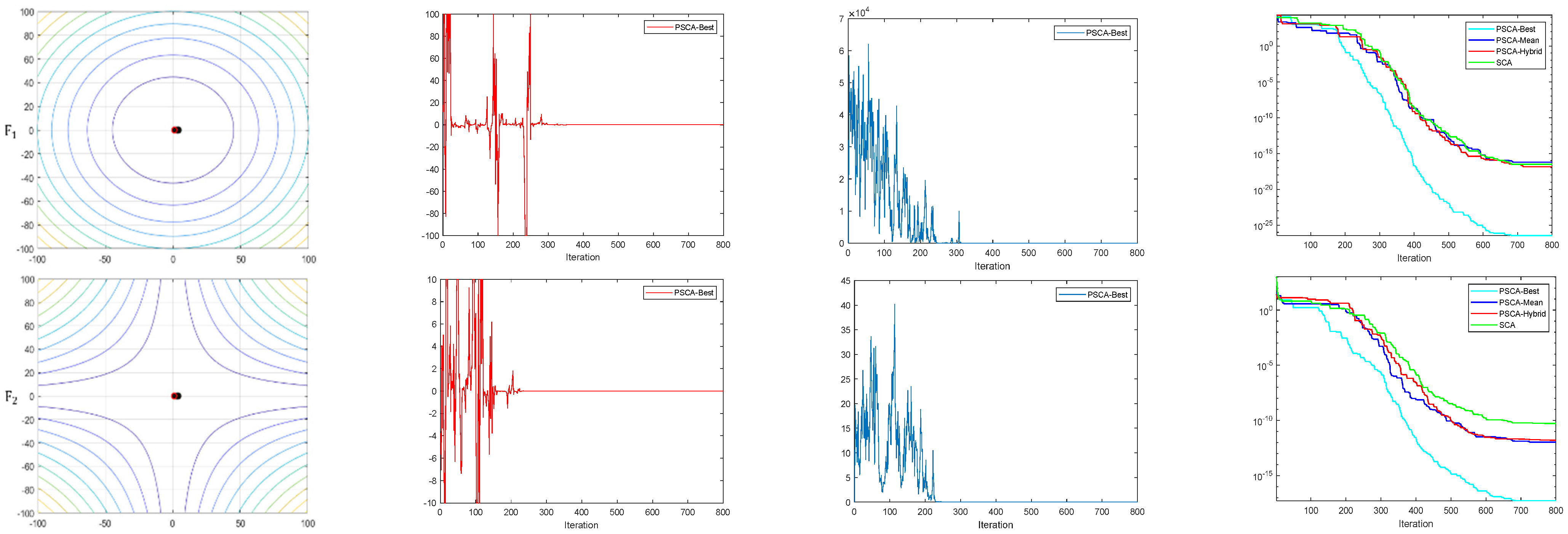
4. The Experiments and Results of the TPSCA

To verify the performance of the TPSCA proposed in this paper, we will conduct comparative experiments with native SCA, PPSO [48] and PMVO [49] based on 23 benchmark functions, $F1~F7$ are unimodal functions, and $F8~F13$ are multimodal functions, $F14~F23$ are complex functions, and the experiment results are shown in

Table 7. The results of benchmark by SCA, TPSCA, PPSO and PMVO.

Function	Values	Algorithm
		SCA	TPSCA	PPSO		PMVO
F1	Best	$9.24\times {10}^{-22}$	$\mathbf{1.74}\mathbf{\times }{\mathbf{10}}^{\mathbf{-}\mathbf{27}}$	$7.76\times {10}^1$		${1.3310}^{-3}$
	Avg	$2.87\times {10}^{-14}$	$\mathbf{3.86}\mathbf{\times }{\mathbf{10}}^{\mathbf{-}\mathbf{19}}$	$1.12\times {10}^2$		$8.29\times {10}^{-3}$
	STD	$1.28\times {10}^{-13}$	$\mathbf{1.62}\mathbf{\times }{\mathbf{10}}^{\mathbf{-}\mathbf{18}}$	$2.14\times {10}^1$		$5.01\times {10}^{-3}$
F2	Best	$1.72\times {10}^{-18}$	$\mathbf{5.59}\mathbf{\times }{\mathbf{10}}^{\mathbf{-}\mathbf{21}}$	$3.01\times {10}^1$		$3.50\times {10}^{-1}$
	Avg	$1.49\times {10}^{-11}$	$\mathbf{9.82}\mathbf{\times }{\mathbf{10}}^{\mathbf{-}\mathbf{16}}$	$5.10\times {10}^2$		$4.57\times {10}^3$
	STD	$6.42\times {10}^{-11}$	$\mathbf{2.66}\mathbf{\times }{\mathbf{10}}^{\mathbf{-}\mathbf{15}}$	$1.20\times {10}^3$		$1.97\times {10}^4$
F3	Best	$3.84\times {10}^{-10}$	$\mathbf{3.86}\mathbf{\times }{\mathbf{10}}^{\mathbf{-}\mathbf{14}}$	$7.21\times {10}^1$		$1.79\times {10}^{-2}$
	Avg	$8.77\times {10}^{-3}$	$\mathbf{8.96}\mathbf{\times }{\mathbf{10}}^{\mathbf{-}\mathbf{5}}$	$1.44\times {10}^2$		$6.13\times {10}^{-2}$
	STD	$3.11\times {10}^{-2}$	$\mathbf{4.00}\mathbf{\times }{\mathbf{10}}^{\mathbf{-}\mathbf{4}}$	$3.29\times {10}^1$		$4.77\times {10}^{-2}$
F4	Best	$6.34\times {10}^{-8}$	$\mathbf{1.21}\mathbf{\times }{\mathbf{10}}^{\mathbf{-}\mathbf{9}}$	$4.55$		$3.41\times {10}^{-2}$
	Avg	$2.75\times {10}^{-4}$	$\mathbf{7.47}\mathbf{\times }{\mathbf{10}}^{\mathbf{-}\mathbf{7}}$	$6.10$		$5.65\times {10}^{-2}$
	STD	$4.89\times {10}^{-4}$	$\mathbf{1.52}\mathbf{\times }{\mathbf{10}}^{\mathbf{-}\mathbf{6}}$	$9.04\times {10}^{-1}$		$1.43\times {10}^{-2}$
F5	Best	$6.93$	$\mathbf{6.46}$	$9.74\times {10}^4$		$7.13$
	Avg	$7.62$	$\mathbf{7.18}$	$2.05\times {10}^5$		$6.60\times {10}^2$
	STD	$\mathbf{3.98}\mathbf{\times }{\mathbf{10}}^{\mathbf{-}\mathbf{1}}$	$4.90\times {10}^{-1}$	$8.64\times {10}^4$		$1.56\times {10}^3$
F6	Best	$2.16\times {10}^{-1}$	$6.46\times {10}^{-2}$	$\mathbf{2.46}\mathbf{\times }{\mathbf{10}}^{\mathbf{-}\mathbf{3}}$		$4.94\times {10}^1$
	Avg	$5.02\times {10}^{-1}$	$3.55\times {10}^{-1}$	$\mathbf{5.55}\mathbf{\times }{\mathbf{10}}^{\mathbf{-}\mathbf{3}}$		$1.05\times {10}^2$
	STD	$1.51\times {10}^{-1}$	$1.43\times {10}^{-1}$	$\mathbf{2.16}\mathbf{\times }{\mathbf{10}}^{\mathbf{-}\mathbf{3}}$		$3.81\times {10}^1$
F7	Best	$2.20\times {10}^{-4}$	$\mathbf{1.53}\mathbf{\times }{\mathbf{10}}^{\mathbf{-}\mathbf{4}}$	$3.39\times {10}^3$		$1.39\times {10}^{-2}$
	Avg	$2.19\times {10}^{-3}$	$\mathbf{1.97}\mathbf{\times }{\mathbf{10}}^{\mathbf{-}\mathbf{3}}$	$1.64\times {10}^4$		$4.38\times {10}^{-2}$
	STD	$\mathbf{1.06}\mathbf{\times }{\mathbf{10}}^{\mathbf{-}\mathbf{3}}$	$1.67\times {10}^{-3}$	$8.90\times {10}^3$		$2.81\times {10}^{-2}$
F8	Best	$-2.44\times {10}^3$	$\mathbf{-}\mathbf{2.56}\mathbf{\times }{\mathbf{10}}^{\mathbf{3}}$	$-5.49\times {10}^2$		$-6.36\times {10}^2$
	Avg	$-2.09\times {10}^3$	$\mathbf{-}\mathbf{2.15}\mathbf{\times }{\mathbf{10}}^{\mathbf{3}}$	$-4.59\times {10}^2$		$-5.34\times {10}^2$
	STD	$1.87\times {10}^2$	$1.96\times {10}^2$	$8.48\times {10}^1$		$\mathbf{7.10}\mathbf{\times }{\mathbf{10}}^{\mathbf{1}}$
F9	Best	$2.12\times {10}^1$	$\mathbf{2.70}\mathbf{\times }{\mathbf{10}}^{\mathbf{-}\mathbf{13}}$	$1.60\times {10}^2$		$1.11\times {10}^1$
	Avg	$4.82\times {10}^1$	$\mathbf{2.62}\mathbf{\times }{\mathbf{10}}^{\mathbf{-}\mathbf{1}}$	$2.03\times {10}^2$		$2.63\times {10}^1$
	STD	$1.16\times {10}^1$	$\mathbf{9.48}\mathbf{\times }{\mathbf{10}}^{\mathbf{-}\mathbf{1}}$	$2.65\times {10}^1$		$1.06\times {10}^1$
F10	Best	$8.63$	$\mathbf{1.01}\mathbf{\times }{\mathbf{10}}^{\mathbf{-}\mathbf{8}}$	$1.09\times {10}^1$		$2.00\times {10}^1$
	Avg	$1.18\times {10}^1$	$\mathbf{4.81}\mathbf{\times }{\mathbf{10}}^{\mathbf{-}\mathbf{3}}$	$1.66\times {10}^1$		$2.01\times {10}^1$
	STD	$1.61$	$2.13\times {10}^{-2}$	$4.28$		$\mathbf{1.58}\mathbf{\times }{\mathbf{10}}^{\mathbf{-}\mathbf{2}}$
F11	Best	$5.36$	$\mathbf{1.39}\mathbf{\times }{\mathbf{10}}^{\mathbf{-}\mathbf{10}}$	$4.92\times {10}^{-1}$		$1.05\times {10}^{-1}$
	Avg	$1.29\times {10}^1$	$\mathbf{6.52}\mathbf{\times }{\mathbf{10}}^{\mathbf{-}\mathbf{2}}$	$7.79\times {10}^{-1}$		$2.53\times {10}^{-1}$
	STD	$5.50$	$\mathbf{9.12}\mathbf{\times }{\mathbf{10}}^{\mathbf{-}\mathbf{2}}$	$1.06\times {10}^{-1}$		$1.31\times {10}^{-1}$
F12	Best	$1.08\times {10}^1$	$\mathbf{5.02}\mathbf{\times }{\mathbf{10}}^{\mathbf{-}\mathbf{2}}$	$6.26$		$5.64$
	Avg	$4.03\times {10}^{-2}$	$\mathbf{1.09}\mathbf{\times }{\mathbf{10}}^{\mathbf{-}\mathbf{1}}$	$9.21$		$6.51\times {10}^6$
	STD	$8.01\times {10}^2$	$\mathbf{3.65}\mathbf{\times }{\mathbf{10}}^{\mathbf{-}\mathbf{2}}$	$1.92$0		$2.91\times {10}^7$
F13	Best	$2.25\times {10}^4$	$\mathbf{4.30}\mathbf{\times }{\mathbf{10}}^{\mathbf{-}\mathbf{3}}$	$1.26\times {10}^1$		$2.35\times {10}^{-1}$
	Avg	$6.49\times {10}^5$	$\mathbf{2.56}\mathbf{\times }{\mathbf{10}}^{\mathbf{-}\mathbf{2}}$	$2.36\times {10}^7$		$3.79\times {10}^{-1}$
	STD	$9.01\times {10}^5$	$\mathbf{1.33}\mathbf{\times }{\mathbf{10}}^{\mathbf{-}\mathbf{2}}$	$1.06\times {10}^8$		$7.30\times {10}^{-2}$
F14	Best	$\mathbf{9.98}\mathbf{\times }{\mathbf{10}}^{\mathbf{-}\mathbf{1}}$	$\mathbf{9.98}\mathbf{\times }{\mathbf{10}}^{\mathbf{-}\mathbf{1}}$	$\mathbf{9.98}\mathbf{\times }{\mathbf{10}}^{\mathbf{-}\mathbf{1}}$		$\mathbf{9.98}\mathbf{\times }{\mathbf{10}}^{\mathbf{-}\mathbf{1}}$
	Avg	$2.88$	$\mathbf{1.06}$	$1.64$		$2.09$
	STD	$2.05$	$\mathbf{1.69}\mathbf{\times }{\mathbf{10}}^{\mathbf{-}\mathbf{1}}$	$9.25\times {10}^{-1}$		$1.50$
F15	Best	$7.37\times {10}^{-4}$	$\mathbf{5.03}\mathbf{\times }{\mathbf{10}}^{\mathbf{-}\mathbf{4}}$	$1.07\times {10}^{-3}$		$1.01\times {10}^{-3}$
	Avg	$1.22\times {10}^{-3}$	$\mathbf{9.43}\mathbf{\times }{\mathbf{10}}^{\mathbf{-}\mathbf{4}}$	$4.86\times {10}^{-3}$		$4.01\times {10}^{-3}$
	STD	$3.52\times {10}^{-4}$	$\mathbf{3.40}\mathbf{\times }{\mathbf{10}}^{\mathbf{-}\mathbf{4}}$	$9.99\times {10}^{-3}$		$7.72\times {10}^{-3}$
F16	Best	$\mathbf{-}\mathbf{1.03}$	$\mathbf{-}\mathbf{1.03}$	$\mathbf{-}\mathbf{1.03}$		$\mathbf{-}\mathbf{1.03}$
	Avg	$\mathbf{-}\mathbf{1.03}$	$\mathbf{-}\mathbf{1.03}$	$-7.49\times {10}^{-1}$		$\mathbf{-}\mathbf{1.03}$
	STD	$9.31\times {10}^{-5}$	$\mathbf{5.47}\mathbf{\times }{\mathbf{10}}^{\mathbf{-}\mathbf{5}}$	$2.16\times {10}^{-1}$		$1.01\times {10}^{-3}$
F17	Best	$3.98\times {10}^{-1}$	$\mathbf{3.98}\mathbf{\times }{\mathbf{10}}^{\mathbf{-}\mathbf{1}}$	$3.98\times {10}^{-1}$		$3.98\times {10}^{-1}$
	Avg	$4.04\times {10}^{-1}$	$\mathbf{4.00}\mathbf{\times }{\mathbf{10}}^{\mathbf{-}\mathbf{1}}$	$5.12\times {10}^{-1}$		$7.12\times {10}^{-1}$
	STD	$8.61\times {10}^{-3}$	$\mathbf{1.42}\mathbf{\times }{\mathbf{10}}^{\mathbf{-}\mathbf{3}}$	$3.39\times {10}^{-1}$		$6.13\times {10}^{-1}$
F18	Best	$\mathbf{3.00}$	$\mathbf{3.00}$	$3.86$		$\mathbf{3.00}$
	Avg	$\mathbf{3.00}$	$\mathbf{3.00}$	$6.26\times {10}^1$		$3.02$
	STD	$7.54\times {10}^{-4}$	$\mathbf{3.90}\mathbf{\times }{\mathbf{10}}^{\mathbf{-}\mathbf{4}}$	$6.48\times {10}^1$		$1.13\times {10}^{-2}$
F19	Best	$\mathbf{-}\mathbf{3.86}$	$\mathbf{-}\mathbf{3.86}$	$-2.73$		$\mathbf{-}\mathbf{3.86}$
	Avg	$-3.85$	$-3.86$	$-2.62\times {10}^{-1}$		$-2.09$
	STD	$6.99\times {10}^{-3}$	$\mathbf{3.81}\mathbf{\times }{\mathbf{10}}^{\mathbf{-}\mathbf{3}}$	$6.46\times {10}^{-1}$		$1.94$
F20	Best	$-3.11$	$\mathbf{-}\mathbf{3.12}$	$-2.35\times {10}^{-29}$		$0.00$
	Avg	$-2.92$	$\mathbf{-}\mathbf{3.05}$	$-1.17\times {10}^{-30}$		$0.00$
	STD	$3.11\times {10}^{-1}$	$4.34\times {10}^{-2}$	$5.25\times {10}^{-30}$		$\mathbf{0.00}$
F21	Best	$-4.93$	$\mathbf{-}\mathbf{1.01}\mathbf{\times }{\mathbf{10}}^{\mathbf{1}}$	$-1.74$		$-8.25$
	Avg	$-1.82$	$\mathbf{-}\mathbf{6.27}$	$-6.14\times {10}^{-1}$		$-3.82$
	STD	$1.50$	$\mathbf{1.49}\mathbf{\times }{\mathbf{10}}^{\mathbf{-}\mathbf{1}}$	$3.29\times {10}^{-1}$		$3.19$
F22	Best	$-4.76$	$\mathbf{-}\mathbf{1.04}\mathbf{\times }{\mathbf{10}}^{\mathbf{1}}$	$-2.05$		$-5.56$
	Avg	$-3.02$	$\mathbf{-}\mathbf{8.68}$	$-9.52\times {10}^{-1}$		$-3.96$
	STD	$1.44$	$\mathbf{1.20}\mathbf{\times }{\mathbf{10}}^{\mathbf{-}\mathbf{2}}$	$4.38\times {10}^{-1}$		$2.78$
F23	Best	$-4.60$	$\mathbf{-}\mathbf{1.05}\mathbf{\times }{\mathbf{10}}^{\mathbf{1}}$	$-2.97$		$-6.43$
	Avg	$-2.55$	$\mathbf{-}\mathbf{8.30}$	$-1.19$		$-4.65$
	STD	$1.13$	$\mathbf{1.49}\mathbf{\times }{\mathbf{10}}^{\mathbf{-}\mathbf{1}}$	$6.02\times {10}^{-1}$		$3.16$
Statistics of the number of wins	Algorithm	Best	Avg		STD
	SCA	4	2		1
	TPSCA	22	22		17
	PPSO	3	1		1
	PMVO	4	0		3

Note: Bold numbers represent the best value for each indicator.

. The experiments in this paper were all performed on the desktop based on Windows 10. The hardware included 64GB RAM, Intel(R) Core (TM) i7-10700KF CPU, and an NVIDIA GeForce RTX 2060 GPU.

The experimental results show that TPSCA exhibited top-notch optimization capabilities, achieving an overwhelming victory. Bold numbers indicate the best results in each group of tests; TPSCA achieved 22 best results in 23 benchmark tests and achieved first place 17 times in standard deviation comparisons. It proves that the TPSCA proposed in this paper has superior performance and reliable stability, and has an average performance improvement of 80% compared with the native SCA.

The experimental results show that TPSCA had an excellent optimization ability and achieved an overwhelming victory. We used Kruskal–Wallis H tests and Friedman M tests to evaluate the four algorithms objectively and comprehensively. The Kruskal–Wallis H test is a nonparametric statistical test that assesses whether the population distributions of multiple independent samples are different.

Table 8. The result of the Kruskal–Wallis H test.

Source	SS	df	Ms	Chi-sq	Prob < Chi-sq
Groups	$3.0776\times {10}^8$	3.0	$1.0259\times {10}^8$	0.94	0.044
Error	$9.5598\times {10}^9$	88	$1.0863\times {10}^8$
Total	$9.8676\times {10}^9$	91

shows the Kruskal–Wallis test results. The p-value obtained was 0.044 (p ≤ 0.05), which means that the test of the result rejected the null hypothesis. Notably, we assumed that the results of the four algorithms followed the same distribution. The Friedman M test is a non-parametric test for multiple related samples, assuming that the optimal distribution of the four algorithms is the same. The test results are shown in

Table 9. The result of the Friedman M test.

Source	SS	df	Ms	Chi-sq	Prob < Chi-sq
Groups	53.47	3.0	17.82	38.44	$2.28\times {10}^{-8}$
Error	42.52	66	0.64
Total	96	91

, the obtained p-value was $2.28\times {10}^{-8}$ $\left(p\le 0.01\right)$, which indicates the significance of the obtained results. The results of both tests confirm the validity and superiority of the proposed approach in achieving the optimum results.

5. Combination of TPSCA and PCNN (TPSCA–PCNN)

Image segmentation technology plays an essential role in remote sensing image processing [50]. Scientific and reasonable image segmentation can provide a good foundation for subsequent advanced image processing and improve the accuracy of target image recognition.

Although PCNNs are widely used in image segmentation, the setting of PCNN model parameters significantly influences the effect of image segmentation. To avoid the under-segmentation or over-segmentation of images due to improper parameter settings [51], in this study, TPSCA was used to optimize three key parameters of PCNN, including link factor, threshold decay factor, and threshold amplification factor. This achieved the acquisition of optimal parameters or near-optimal parameters, and improved the segmentation effect of remote sensing images. The flowchart of the TPSCA–PCNN image segmentation model is shown in Figure 6.

6. Remote Sensing Image Segmentation Model Based on TPSCA–PCNN

6.1. Image Segmentation Evaluation Metrics

To evaluate the optimization effect of TPSCA on PCNN, the fitness function was the accuracy rate (ACC), which is shown in Equation (10). The closer the result of is ACC to 100%, the better image segmentation will be achieved.

$$fitness=ACC=\frac{TP+TN}{FN+FP+TP+TN}$$

(10)

where $TP$ is true positive, $TN$ is true negative, $FP$ is false positive, and $FN$ is false negative.

To evaluate the image segmentation effect more comprehensively, we also used sensitivity ($Sen$), precision ($Pre$), Matthews correlation coefficient ($MCC$), Jaccard similarity coefficient (Jac), and specificity ($Spe$) indicators to evaluate the image segmentation effect. Among them, $Sen$ and $Spe$ together reflect the pixel error of the segmentation model: the closer they are to 100%, the better the segmentation effect of the model; $Pre$ represents the correct rate of image segmentation; $MCC$ is the correlation coefficient between the segmentation result and the segmented image, with a range of [−1, 1]. A value of MCC equal to 1 indicates that the image is perfectly segmented, whereas a value of −1 indicates that the image is completely incorrectly segmented. $Jac$ is used to compare the similarities and differences between original image and segmented image; nearer 100% means a better image segmentation effect. The calculation methods of the above indicators are shown in Equations (11)–(16):

$$Sen=\frac{TP}{TP+FN}$$

(11)

$$Pre=\frac{TP}{TP+FP}$$

(12)

$$MCC=\frac{TP\times TN-FP\times FN}{\sqrt{\left(\left(TP+FP\right)\times \left(TP+FN\right)\times \left(TN+FP\right)\times \left(TN+FN\right)\right)}}$$

(13)

$$Dice=\frac{2\times TP}{2\times TP+FP+FN}$$

(14)

$$Jac=\frac{Dice}{2-Dice}$$

(15)

$$Spe=\frac{TN}{TN+FP}$$

(16)

6.2. Remote Sensing Image Datasets

The images used for the simulation experiments in this paper were all from remote sensing image datasets. The images were selected from the IKONOS, GeoEye-1, and WorldView-2 satellite remote sensing image datasets. The available bands of the GeoEye-1 satellite are panchromatic bands with a spatial resolution of 0.50 m and four multispectral bands (blue, green, red, and NIR) with a spatial resolution of 2.00 m, and the image coverage area is 10 × 10 km bands (blue, green, red, and NIR). WorldView-2 also scans in the yellow (585~625 nm), NIR-2 (860~1040 nm), and coastal blue (400~450 nm) spectral ranges, with an image coverage area of 17.64 × 17.64 km.

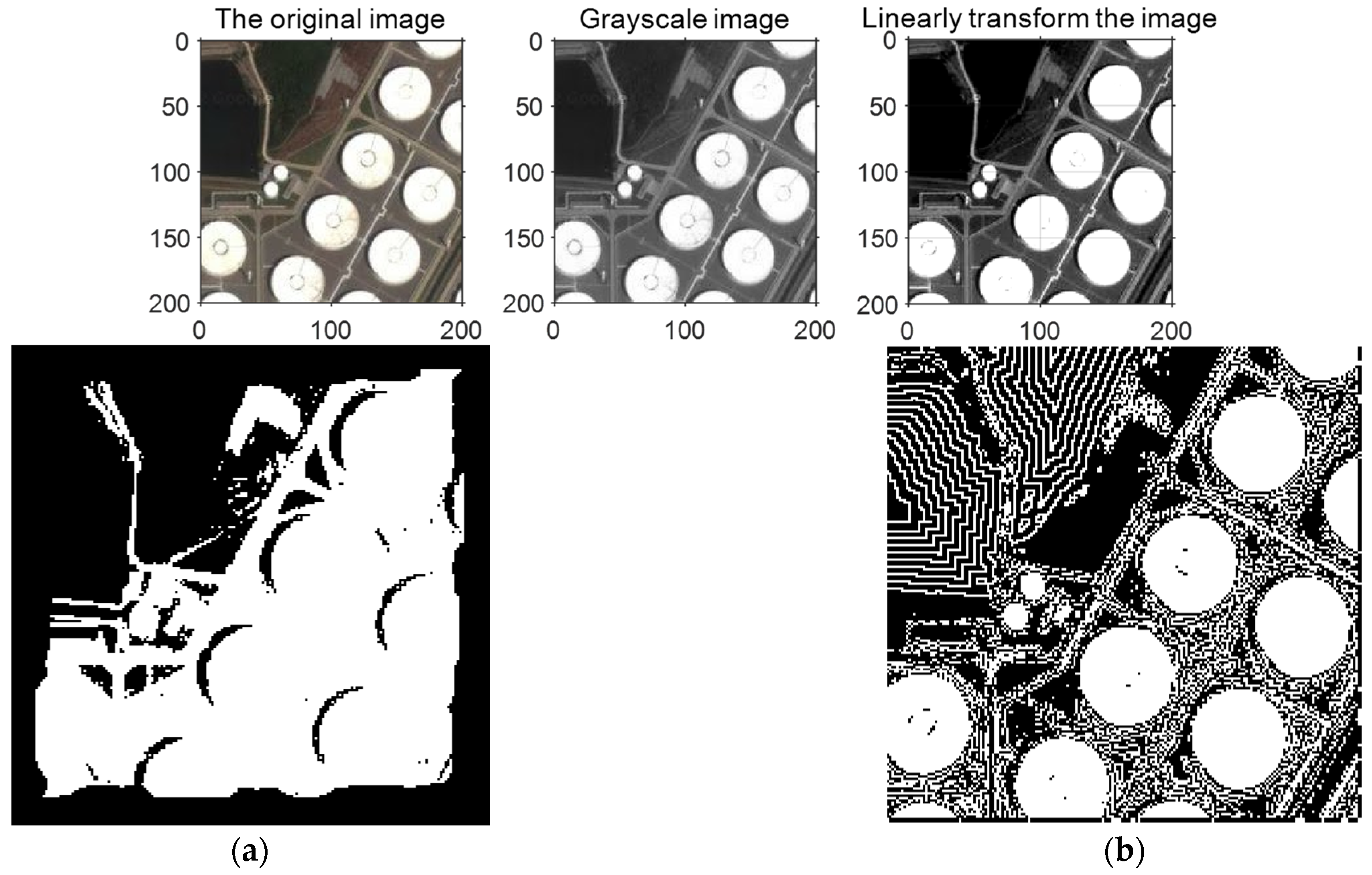
6.3. Image Preprocessing

Before image segmentation, images were preprocessed to enhance the detectability of relevant information and simplify image information [52]. In this study, we used image linear transform to preprocess the image to be segmented and enhance the contrast between the parts of the image to be segmented in order to correct random errors in the process of image feature acquisition. In addition, in order to improve the processing speed of the model, this study used the weighted average method for image grayscale processing for color images. The comparison of image segmentation effects regarding the original image and after preprocessing is presented in Figure 7, which clearly shows the necessity and importance of preprocessing for image segmentation.

To verify the segmentation effect of TPSCA–PCNN on remote sensing images, in this study, a series of simulation experiments were conducted, and the original PCNN and extreme learning machine (ELM) [53] were added to the comparison experiments. Image 1 and Image 2 were selected from the IKONOS satellite remote sensing image; Image 3 and Image 4 were selected from the GeoEye-1 satellite remote sensing image; Image 5 and Image 6 were selected from the WorldView-2 satellite remote sensing image; the segmentation effects are shown in Figure 8, Figure 9, Figure 10, Figure 11, Figure 12 and Figure 13; the experimental results are shown in

Table 10. The experimental results of image segmentation using TPSCA–PCNN, PCNN, and ELM.

Dataset	Model	Evaluation Metrics
		$\mathit{A}\mathit{C}\mathit{C}$	$\mathit{S}\mathit{e}\mathit{n}$	$\mathit{P}\mathit{r}\mathit{e}$	$\mathit{M}\mathit{C}\mathit{C}$	$\mathit{J}\mathit{a}\mathit{c}$	$\mathit{S}\mathit{p}\mathit{e}$
Image 1	TPSCA–PCNN	88.25%	96.28%	79.79%	77.69%	77.40%	82.48%
	PCNN	43.98%	42.87%	35.81%	−12.19%	24.24%	44.77%
	ELM	13.52%	10.57%	8.26%	−72.98%	4.86%	15.64%
Image 2	TPSCA–PCNN	95.83%	99.29%	99.28%	91.88%	91.68%	92.85%
	PCNN	35.45%	4.95%	10.00%	−39.65%	3.42%	61.64%
	ELM	48.99%	48.97%	45.28%	−2.01%	30.77%	49.01%
Image 3	TPSCA–PCNN	85.13%	99.59%	70.40%	73.41%	70.02%	77.28%
	PCNN	43.42%	40.47%	28.54%	−13.86%	20.10%	45.02%
	ELM	25.47%	32.07%	45.28%	−45.28%	13.15%	21.89%
Image 4	TPSCA–PCNN	86.16%	99.79%	40.64%	50.27%	40.59%	62.56%
	PCNN	38.68%	22.18%	9.06%	−2.82%	6.88%	42.24%
	ELM	26.83%	0.56%	2.08%	−50.35%	1.54%	32.27%
Image 5	TPSCA–PCNN	84.59%	89.69%	72.19%	64.44%	61.69%	73.24%
	PCNN	10.91%	2.67%	0.22%	−79.39%	1.22%	16.69%
	ELM	11.77%	5.03%	4.52%	−77.11%	2.58%	16.06%
Image 6	TPSCA–PCNN	85.67%	99.70%	71.54%	74.36%	71.38%	77.83%
	PCNN	54.31%	23.69%	31.66%	−5.29%	15.68%	71.42%
	ELM	71.37%	79.85%	57.22%	44.56%	50.00%	66.63%

Note: The bold numbers represent the best value for each indicator.

.

From the segmentation results of the six remotely sensed images, it can be intuitively seen that the segmentation effect of TPSCA–PCNN is the most satisfying and significantly better than the other two models. Some indicators of PCNN in processing Image 2, Image 3, Image 5, and Image 6 are worse than ELM, but after TPSCA optimization, the under-segmentation of PCNN is successfully solved. The TPSCA–PCNN model proposed in this paper is significantly better than others. In the evaluation of $Sen$ and $Spe$, the $Sen$ of the TPSCA–PCNN model is close to 100%, and $Spe$ also has obvious advantages compared with other models; in the ranking of $ACC$, $MCC$, and $Jac$, TPSCA–PCNN was clearly the best. Although the time complexity of the TPSCA–PCNN proposed in this paper is higher than that of the native PCNN, the segmentation performance has a nearly 40% improvement compared with the initial PCNN model. Additionally, the comprehensive evaluation of various metrics shows that the image segmentation model proposed in this paper performs well.

7. Conclusions

Efficient and accurate image segmentation model plays an important role in the analysis and utilization of remote sensing images. In this paper, we have proposed a customized parallel SCA based on the Taguchi method (TPSCA). The Taguchi-legislated optimal parallelism scheme was used to provide a scientific, rational, and efficient design solution for parallel algorithm design. The optimized performance of TPSCA was verified using 23 benchmark functions. The PCNN optimized by TPSCA successfully completed the task of remote sensing segmentation, showing its application potential and practical value in this field.

Time complexity is an evaluation indicator to measure the merit of an algorithm. The time complexity of the TPSCA proposed in this paper consists of three parts: Taguchi’s method customizing the parallel solution, initialization, and updating the solution. The time complexity of the Taguchi method is $\mathrm{O}\left(1\right)$. The time complexity of the initialization process is $\mathrm{O}\left(\mathrm{G}\times \mathrm{N}/\mathrm{G}\right)$, where $\mathrm{N}$ is the population size and $\mathrm{G}$ is the number of groups; because this study adopted a parallel strategy, no matter how many groups were divided did not change the population size $\mathrm{N}$. The time complexity of the update solution process is $\mathrm{O}\left(\mathrm{N}\times \mathrm{T}\right)+\mathrm{O}\left(\mathrm{N}\times \mathrm{D}\times \mathrm{T}\right)$, where $\mathrm{T}$ denotes the total number of iterations and $\mathrm{D}$ denotes the dimensionality. The time complexity of the TPSCA is $\mathrm{O}\left( \mathrm{I}{\left(\mathrm{NK}\right)}^3 \right)$, where $\mathrm{I}$ is the number of iterations and $\mathrm{NK}$ denotes the number of updated variables, which is the same as the SCA.

In this study, although the stochastic nature of the metaheuristic algorithm could determine the optimal threshold more efficiently, there are inevitably drawbacks, such as increased arithmetic power demand and long computation time. Therefore, in future research, we will consider the use of surrogate techniques to improve the metaheuristic algorithm [54,55] to increase the computational speed. Additionally, we will continue to explore more integrated uses of multiple intelligent techniques in remote sensing image processing.

References

1. Song, J.; Gao, S.; Zhu, Y.; Ma, C. A Survey of Remote Sensing Image Classification Based on CNNs. Big Earth Data 2019, 3, 232–254. [Google Scholar] [CrossRef]
2. Prabhu, R.; Alagu Raja, R.A. Urban Slum Detection Approaches from High-Resolution Satellite Data Using Statistical and Spectral Based Approaches. J. Indian Soc. Remote Sens. 2018, 46, 2033–2044. [Google Scholar] [CrossRef]
3. Lian, J.; Yang, Z.; Liu, J.; Sun, W.; Zheng, L.; Du, X.; Yi, Z.; Shi, B.; Ma, Y. An Overview of Image Segmentation Based on Pulse-Coupled Neural Network. Arch. Comput. Methods Eng. 2021, 28, 387–403. [Google Scholar] [CrossRef]
4. Yokoya, N.; Levine, M.D. Range Image Segmentation Based on Differential Geometry: A Hybrid Approach. J. Indian Soc. Remote Sens. 2018, 46, 2033–2044. [Google Scholar] [CrossRef]
5. Zhang, H.; Liu, M.; Wang, Y.; Shang, J.; Liu, X.; Li, B.; Song, A.; Li, Q. Automated Delineation of Agricultural Field Boundaries from Sentinel-2 Images Using Recurrent Residual U-Net. Int. J. Appl. Earth Obs. Geoinf. 2021, 105, 102557. [Google Scholar] [CrossRef]
6. Mittal, H.; Saraswat, M. An Optimum Multi-Level Image Thresholding Segmentation Using Non-Local Means 2D Histogram and Exponential Kbest Gravitational Search Algorithm. Eng. Appl. Artif. Intell. 2018, 71, 226–235. [Google Scholar] [CrossRef]
7. Kim, W.; Kanezaki, A.; Tanaka, M. Unsupervised Learning of Image Segmentation Based on Differentiable Feature Clustering. IEEE Trans. Image Processing 2020, 29, 8055–8068. [Google Scholar] [CrossRef]
8. Liu, C.; Liu, W.; Xing, W. A Weighted Edge-Based Level Set Method Based on Multi-Local Statistical Information for Noisy Image Segmentation. J. Vis. Commun. Image Represent. 2019, 59, 89–107. [Google Scholar] [CrossRef]
9. Yu, H.; He, F.; Pan, Y. A Scalable Region-Based Level Set Method Using Adaptive Bilateral Filter for Noisy Image Segmentation. Multimed. Tools Appl. 2020, 79, 5743–5765. [Google Scholar] [CrossRef]
10. Alshehhi, R.; Marpu, P.R. Hierarchical Graph-Based Segmentation for Extracting Road Networks from High-Resolution Satellite Images. ISPRS J. Photogramm. Remote Sens. 2017, 126, 245–260. [Google Scholar] [CrossRef]
11. Li, X.; Yang, X.; Li, X.; Lu, S.; Ye, Y.; Ban, Y. Cloud Detection Approach for Remote Sensing Images. Knowl.-Based Syst. 2022, 238, 107890. [Google Scholar] [CrossRef]
12. Mirjalili, S. SCA: A Sine Cosine Algorithm for Solving Optimization Problems. Knowl.-Based Syst. 2016, 96, 120–133. [Google Scholar] [CrossRef]
13. Xia, J.; Yang, D.; Zhou, H.; Chen, Y.; Zhang, H.; Liu, T.; Heidari, A.A.; Chen, H.; Pan, Z. Evolving Kernel Extreme Learning Machine for Medical Diagnosis via a Disperse Foraging Sine Cosine Algorithm. Comput. Biol. Med. 2022, 141, 105137. [Google Scholar] [CrossRef]
14. Zheng, H.; Gao, J.; Xiong, J.; Yao, G.; Cui, H.; Zhang, L. An Enhanced Artificial Electric Field Algorithm with Sine Cosine Mechanism for Logistics Distribution Vehicle Routing. Appl. Sci. 2022, 12, 6240. [Google Scholar] [CrossRef]
15. Elaziz, M.A.; Ewees, A.A.; Al-qaness, M.A.A.; Abualigah, L.; Ibrahim, R.A. Sine–Cosine-Barnacles Algorithm Optimizer with Disruption Operator for Global Optimization and Automatic Data Clustering. Expert Syst. Appl. 2022, 207, 117993. [Google Scholar] [CrossRef]
16. Zhou, Z.; Rahman Siddiquee, M.M.; Tajbakhsh, N.; Liang, J. Unet++: A Nested U-Net Architecture for Medical Image Segmentation. In Lecture Notes in Computer Science (including Subseries Lecture Notes in Artificial Intelligence and Lecture Notes in Bioinformatics); Springer: Berlin/Heidelberg, Germany, 2018; Volume 11045, pp. 3–11. [Google Scholar]
17. Jha, D.; Riegler, M.A.; Johansen, D.; Halvorsen, P.; Johansen, H.D. DoubleU-Net: A Deep Convolutional Neural Network for Medical Image Segmentation. In Proceedings of the IEEE Symposium on Computer-Based Medical Systems, Rochester, MN, USA, 28–30 July 2020; Institute of Electrical and Electronics Engineers Inc.: Piscataway, NJ, USA, 2020; Volume 2020, pp. 558–564. [Google Scholar]
18. Jia, H.; Xing, Z.; Song, W. Three Dimensional Pulse Coupled Neural Network Based on Hybrid Optimization Algorithm for Oil Pollution Image Segmentation. Remote Sens. 2019, 11, 1046. [Google Scholar] [CrossRef]
19. Deng, X.; Yang, Y.; Zhang, H.; Ma, Y. PCNN Double Step Firing Mode for Image Edge Detection. Multimed. Tools Appl. 2022, 81, 27187–27213. [Google Scholar] [CrossRef]
20. Zhou, D.; Shao, Y. Region Growing for Image Segmentation Using an Extended PCNN Model. IET Image Process. 2018, 12, 729–737. [Google Scholar] [CrossRef]
21. Sarkar, S.; Das, S.; Chaudhuri, S.S. Multi-Level Thresholding with a Decomposition-Based Multi-Objective Evolutionary Algorithm for Segmenting Natural and Medical Images. Appl. Soft Comput. J. 2017, 50, 142–157. [Google Scholar] [CrossRef]
22. Zhang, C.; Xie, Y.; Liu, D.; Wang, L. Fast Threshold Image Segmentation Based on 2D Fuzzy Fisher and Random Local Optimized QPSO. IEEE Trans. Image Process. 2017, 26, 1355–1362. [Google Scholar] [CrossRef]
23. Sun, Y.; Chu, S.-C.; Hu, P.; Watada, J.; Si, M.; Pan, J.-S. Overview of Parallel Computing for Meta-Heuristic Algorithms. Taiwan Ubiquitous Inf. 2022, 7, 656–684. [Google Scholar]
24. Fan, F.; Chu, S.C.; Pan, J.S.; Yang, Q.; Zhao, H. Parallel Sine Cosine Algorithm for the Dynamic Deployment in Wireless Sensor Networks. J. Internet Technol. 2021, 22, 499–512. [Google Scholar] [CrossRef]
25. Chu, S.C.; Xu, X.W.; Yang, S.Y.; Pan, J.S. Parallel Fish Migration Optimization with Compact Technology Based on Memory Principle for Wireless Sensor Networks. Knowl.-Based Syst. 2022, 241, 108124. [Google Scholar] [CrossRef]
26. Yang, W.H.; Tarng, Y.S. Design Optimization of Cutting Parameters for Turning Operations Based on the Taguchi Method. J. Mater. Process. Technol. 1998, 84, 122–129. [Google Scholar] [CrossRef]
27. Belazzoug, M.; Touahria, M.; Nouioua, F.; Brahimi, M. An Improved Sine Cosine Algorithm to Select Features for Text Categorization. J. King Saud Univ. Comput. Inf. Sci. 2020, 32, 454–464. [Google Scholar] [CrossRef]
28. Qu, C.; Zeng, Z.; Dai, J.; Yi, Z.; He, W. A Modified Sine-Cosine Algorithm Based on Neighborhood Search and Greedy Levy Mutation. Comput. Intell. Neurosci. 2018, 2018, 4231647. [Google Scholar] [CrossRef] [PubMed]
29. Ji, Y.; Tu, J.; Zhou, H.; Gui, W.; Liang, G.; Chen, H.; Wang, M. An Adaptive Chaotic Sine Cosine Algorithm for Constrained and Unconstrained Optimization. Complexity 2020, 2020, 6084917. [Google Scholar] [CrossRef]
30. Chegini, S.N.; Bagheri, A.; Najafi, F. PSOSCALF: A New Hybrid PSO Based on Sine Cosine Algorithm and Levy Flight for Solving Optimization Problems. Appl. Soft Comput. J. 2018, 73, 697–726. [Google Scholar] [CrossRef]
31. Dey, B.; Bhattacharyya, B. Comparison of Various Electricity Market Pricing Strategies to Reduce Generation Cost of a Microgrid System Using Hybrid WOA-SCA. Evol. Intell. 2021, 15, 1587–1604. [Google Scholar] [CrossRef]
32. Sun, X.; Shi, Z.; Zhu, J. Multiobjective Design Optimization of an IPMSM for EVs Based on Fuzzy Method and Sequential Taguchi Method. IEEE Trans. Ind. Electron. 2021, 68, 10592–10600. [Google Scholar] [CrossRef]
33. Balaram Naik, A.; Chennakeshava Reddy, A. Optimization of Tensile Strength in TIG Welding Using the Taguchi Method and Analysis of Variance (ANOVA). Therm. Sci. Eng. Prog. 2018, 8, 327–339. [Google Scholar] [CrossRef]
34. Tsai, P.W.; Pan, J.S.; Chen, S.M.; Liao, B.Y. Enhanced Parallel Cat Swarm Optimization Based on the Taguchi Method. Expert Syst. Appl. 2012, 39, 6309–6319. [Google Scholar] [CrossRef]
35. Diao, K.; Sun, X.; Lei, G.; Bramerdorfer, G.; Guo, Y.; Zhu, J. Robust Design Optimization of Switched Reluctance Motor Drive Systems Based on System-Level Sequential Taguchi Method. IEEE Trans. Energy Convers. 2021, 36, 3199–3207. [Google Scholar] [CrossRef]
36. Hong, Y.Y.; Beltran, A.A.; Paglinawan, A.C. A Robust Design of Maximum Power Point Tracking Using Taguchi Method for Stand-Alone PV System. Appl. Energy 2018, 211, 50–63. [Google Scholar] [CrossRef]
37. Gao, H.; Zhao, H.; Chen, S. Image Denoising Method of Auto-Evolving PCNN Model Based on Quantum Selfish Herd Algorithm. In Advances in Swarm Intelligence; Springer: Berlin/Heidelberg, Germany, 2022; pp. 128–138. [Google Scholar]
38. Nie, R.; He, M.; Cao, J.; Zhou, D.; Liang, Z. Pulse Coupled Neural Network Based MRI Image Enhancement Using Classical Visual Receptive Field for Smarter Mobile Healthcare. J. Ambient Intell. Humaniz. Comput. 2019, 10, 4059–4070. [Google Scholar] [CrossRef]
39. Panigrahy, C.; Seal, A.; Mahato, N.K. MRI and SPECT Image Fusion Using a Weighted Parameter Adaptive Dual Channel PCNN. IEEE Signal Process. Lett. 2020, 27, 690–694. [Google Scholar] [CrossRef]
40. Deng, X.; Ye, J. A Retinal Blood Vessel Segmentation Based on Improved D-MNet and Pulse-Coupled Neural Network. Biomed. Signal Process. Control 2022, 73, 103467. [Google Scholar] [CrossRef]
41. Deng, X.; Yang, Y.; Sun, H. An Adaptive Threshold Setting Algorithm Based on PCNN Edge Detection Model. In Proceedings of the ACM International Conference Proceeding Series, Association for Computing Machinery, New York, NY, USA, 20 February 2021; pp. 34–41. [Google Scholar]
42. Zhang, D.; Wang, D.; Gu, C.; Jin, N.; Zhao, H.; Chen, G.; Liang, H.; Liang, D. Using Neural Network to Identify the Severity of Wheat Fusarium Head Blight in the Field Environment. Remote Sens. 2019, 11, 2375. [Google Scholar] [CrossRef]
43. Xu, X.; Liang, T.; Wang, G.; Wang, M.; Wang, X. Self-Adaptive PCNN Based on the ACO Algorithm and Its Application on Medical Image Segmentation. Intell. Autom. Soft Comput. 2017, 23, 303–310. [Google Scholar] [CrossRef]
44. Low, K.S.; Zhuang, H. Real Time Runway Detection in Satellite Images Using Multi-Channel PCNN. In Proceedings of the 2014 9th IEEE Conference on Industrial Electronics and Applications, Hangzhou, China, 9–11 June 2014; ISBN 9781479943159. [Google Scholar]
45. Gu, X. Feature Extraction Using Unit-Linking Pulse Coupled Neural Network and Its Applications. Neural Process. Lett. 2008, 27, 25–41. [Google Scholar] [CrossRef]
46. Pan, J.S.; Hu, P.; Chu, S.C. Novel Parallel Heterogeneous Meta-Heuristic and Its Communication Strategies for the Prediction of Wind Power. Processes 2019, 7, 845. [Google Scholar] [CrossRef] [Green Version]
47. Wolpert, D.H.; Macready, W.G. No free lunch theorems for optimization. IEEE Trans. Evol. Comput. 1997, 1, 67–82. [Google Scholar] [CrossRef]
48. Chang, J.-F.; Chu, S.-C.; Roddick, J.F.; Pan, J.-S. A Parallel Particle Swarm Optimization Algorithm with Communication Strategies. J. Inf. Sci. Eng. 2005, 21, 9. [Google Scholar]
49. Wang, X.; Pan, J.S.; Chu, S.C. A Parallel Multi-Verse Optimizer for Application in Multilevel Image Segmentation. IEEE Access 2020, 8, 32018–32030. [Google Scholar] [CrossRef]
50. Zhang, X.; Han, L.; Dong, Y.; Shi, Y.; Huang, W.; Han, L.; González-Moreno, P.; Ma, H.; Ye, H.; Sobeih, T. A Deep Learning-Based Approach for Automated Yellow Rust Disease Detection from High-Resolution Hyperspectral UAV Images. Remote Sens. 2019, 11, 1554. [Google Scholar] [CrossRef]
51. Jia, H.; Peng, X.; Kang, L.; Li, Y.; Jiang, Z.; Sun, K. Pulse Coupled Neural Network Based on Harris Hawks Optimization Algorithm for Image Segmentation. Multimed. Tools Appl. 2020, 79, 28369–28392. [Google Scholar] [CrossRef]
52. Natteshan, N.V.S.; Suresh Kumar, N. Effective SAR Image Segmentation and Classification of Crop Areas Using MRG and CDNN Techniques. Eur. J. Remote Sens. 2020, 53, 126–140. [Google Scholar] [CrossRef]
53. Huang, G.-B.; Zhu, Q.Y.; Siew, C.K. Extreme Learning Machine: Theory and Applications. Neurocomputing 2006, 70, 489–501. [Google Scholar] [CrossRef]
54. Chu, S.-C.; Du, Z.-G.; Peng, Y.-J.; Pan, J.-S. Fuzzy Hierarchical Surrogate Assists Probabilistic Particle Swarm Optimization for Expensive High Dimensional Problem. Knowl.-Based Syst. 2021, 220, 106939. [Google Scholar]
55. Wang, H.; Liang, M.; Sun, C.; Zhang, G.; Xie, L. Multiple-Strategy Learning Particle Swarm Optimization for Large-Scale Optimization Problems. Complex Intell. Syst. 2021, 7, 1–16. [Google Scholar] [CrossRef]
Figure 1. Working principle diagram of the PCNN.
Remotesensing 14 04875 g001
Figure 2. Execution flow of Strategy 1.
Remotesensing 14 04875 g002
Figure 3. Execution flow of Strategy 2.
Remotesensing 14 04875 g003
Figure 4. Optimization results of the benchmark: (a) 2D position distribution; (b) Trajectory in the first dimension; (c) Average fitness; (d) Convergence curves.
Remotesensing 14 04875 g004aRemotesensing 14 04875 g004b
Figure 5. Signal-to-noise ratio main effect map: (a) the SNR main effect graph of unimodal function F 2 ; (b) the SNR main effect graph of multimodal function F 12 ; (c) the SNR main effect graph of complex function F 18 .
Remotesensing 14 04875 g005
Figure 6. Flowchart of TPSCA–PCNN.
Remotesensing 14 04875 g006
Figure 7. Comparison of image segmentation effects before and after preprocessing: (a) before image preprocessing; (b) after image preprocessing.
Remotesensing 14 04875 g007
Figure 8. Segmentation results of IKONOS satellite remote sensing image 1: (a) original remote sensing image; (b) TPSCA–PCNN segmentation result; (c) PCNN segmentation result; (d) ELM segmentation result.
Remotesensing 14 04875 g008
Figure 9. Segmentation results of IKONOS satellite remote sensing image 2: (a) original remote sensing image; (b) TPSCA–PCNN segmentation result; (c) PCNN segmentation result; (d) ELM segmentation result.
Remotesensing 14 04875 g009
Figure 10. Segmentation results of GeoEye-1 satellite remote sensing image 3: (a) original remote sensing image; (b) TPSCA–PCNN segmentation result; (c) PCNN segmentation result; (d) ELM segmentation result.
Remotesensing 14 04875 g010
Figure 11. Segmentation results of GeoEye-1 satellite remote sensing image 4: (a) original remote sensing image; (b) TPSCA–PCNN segmentation result; (c) PCNN segmentation result; (d) ELM segmentation result.
Remotesensing 14 04875 g011
Figure 12. Segmentation results of WorldView-2 satellite remote sensing image 5: (a) original remote sensing image; (b) TPSCA–PCNN segmentation result; (c) PCNN segmentation result; (d) ELM segmentation result.
Remotesensing 14 04875 g012
Figure 13. Segmentation results of WorldView-2 satellite remote sensing image 6: (a) original remote sensing image; (b) TPSCA–PCNN segmentation result; (c) PCNN segmentation result; (d) EML segmentation result.
Remotesensing 14 04875 g013