Article

The Self-Supervised Spectral–Spatial Vision Transformer Network for Accurate Prediction of Wheat Nitrogen Status from UAV Imagery

1
Department of Computing and Mathematics, Manchester Metropolitan University, Manchester M15GD, UK
2
GMV, Glasgow, Scotland G431QQ, UK
3
Department of Health Studies, Royal Holloway, University of London, Egham TW200EX, UK
4
Bockhanger Farms Ltd., Oaklands Farm, Ashford TN261ER, UK
*
Author to whom correspondence should be addressed.
Remote Sens. 2022, 14(6), 1400; https://doi.org/10.3390/rs14061400
Submission received: 27 January 2022 / Revised: 4 March 2022 / Accepted: 8 March 2022 / Published: 14 March 2022

Abstract

:
Nitrogen (N) fertilizer is routinely applied by farmers to increase crop yields. At present, farmers often over-apply N fertilizer in some locations or at certain times because they do not have high-resolution crop N status data. N-use efficiency can be low, with the remaining N lost to the environment, resulting in higher production costs and environmental pollution. Accurate and timely estimation of N status in crops is crucial to improving cropping systems’ economic and environmental sustainability. Destructive approaches based on plant tissue analysis are time consuming and impractical over large fields. Recent advances in remote sensing and deep learning have shown promise in addressing the aforementioned challenges in a non-destructive way. In this work, we propose a novel deep learning framework: a self-supervised spectral–spatial attention-based vision transformer (SSVT). The proposed SSVT introduces a Spectral Attention Block (SAB) and a Spatial Interaction Block (SIB), which allows for simultaneous learning of both spatial and spectral features from UAV digital aerial imagery, for accurate N status prediction in wheat fields. Moreover, the proposed framework introduces local-to-global self-supervised learning to help train the model from unlabelled data. The proposed SSVT has been compared with five state-of-the-art models including: ResNet, RegNet, EfficientNet, EfficientNetV2, and the original vision transformer on both testing and independent datasets. The proposed approach achieved high accuracy (0.96) with good generalizability and reproducibility for wheat N status estimation.

1. Introduction

Nitrogen is an essential plant nutrient and is vital for plant growth and development. The application of N fertilizers has revolutionized farming, increasing crop yields and food production to meet the nutritional needs of billions of people. It is estimated that global nitrogen fertilizer demand was 110 million tonnes (MT) in 2015 and is projected to be 120 MT in 2020, costing farmers over USD 100 billion per year [1,2]. Optimal application of N fertilizers enhances soil fertility and increases crop yields. On the other hand, excessive N inputs are costly for farmers but do not deliver any additional yield benefits, instead resulting in the pollution of natural ecosystems, increases in emissions of the potent greenhouse gas nitrous oxide, and reductions in biodiversity [3,4]. Wheat crops invariably require fertilizer to grow optimally and are the world’s most commonly consumed cereal grain and one of the worldwide staple foods. About 35–40% of the global population depend on wheat as their major food crop [5]. Accurate monitoring of the N status in wheat informs farmer decisions on nitrogen fertilizer application rates and timing. It is therefore crucial for the economic and environmental sustainability of cropping systems to support a secure food supply chain.
Many crop N estimation methods have been proposed which can be broadly divided into two approaches: destructive and non-destructive. The destructive methods are mostly based on tissue analysis of plant leaves in the laboratory and are time-consuming and costly, which is impractical when collecting the data over large areas [3,6]. In contrast, non-destructive methods perform estimation proximally and remotely of the crop’s N status, in a timely fashion and without causing damage to the plants.
Recently, with the development of remote sensing technology, the optical sensors mounted on unmanned aerial vehicles (UAV), aeroplanes, and satellites provide a non-destructive, rapid, and relatively inexpensive crop N estimation method. These sensors, such as RGB sensors and multi to hyperspectral sensors, capture the data remotely to measure the radiation reflected by plants [7]. The optical sensors can provide rich spectral information in different spectrum regions, including the visible region (380–700 nm, VIS), the near infrared region (700–1300 nm, NIR) and the shortwave infrared region (1300–2500 nm, SWIR). The spectral information in these regions is considered to indirectly estimate the biological (e.g., photo- synthetic pigments, chlorophylls) and morphological (leaf area, canopy density) features of the crop and thus derive the N content and status [3]. In general, the measurements from these sensors provides a cubic data format containing spatial information in two dimensions (X–Y axis) and abundant spectral information in the third dimension (Z axis). Depending on the dimensions of the data used, we can classify the estimation methods into two categories: spectral analysis and spatial analysis.
The spectral analysis methods in remote sensing applications assume that the spectral information of each pixel can be used to measure the objectives, such as the N content of the crop [8]. One of the most commonly used spectral analysis methods is to use vegetation indexes (VI) based on specific wavelengths to predict the crop N content and status, such as Normalized Difference Vegetation Index (NDVI) [9] and canopy chlorophyll content index (CCCI) [10]. However, the indirect determination of N content of crops from remotely sensed data is considered a complex problem, which is affected by various influential factors such as ambient lighting conditions and variations amongst the types of crops. The VI methods based on specific wavelengths are considered sensitive and lack generalizability [11]. Machine learning has shown the effectiveness of solving nonlinear problems from multiple sources [12], and in recent years has been increasingly used for crop N estimation. In [13,14], the author used three machine learning algorithms (Random Forest (RF), Support Vector Machine (SVM), and Artificial Neural Networks (ANNs)) to estimate rice nitrogen based on all available spectral information, with the random forest (RF) demonstrating high accuracy and strong generalization performance.
With advancements in remote sensing, the resolution of the data, including the spatial and spectral, has been significantly improved. The variation in spectral features between neighbouring pixels increases as the spatial resolution is improved [15]. The spatial information in the finer spatial resolution data can be used to measure the structure and health condition of the crop; these are considered essential attributes for characterizing the N status [16]. However, conventional spectral-based VI methods have difficulty in analysing high spatial resolution data, with few works using spatial information for crop N estimation [16]. Accurate estimation of crop N content incorporating spatial information remains a challenge.
Over the past few years, with the emergence of graphic processing units (GPU) [17], deep learning (DL) methods, have dominated computer vision tasks and are considered superior to pre-existing methods for extracting spatial features from images [18]. They are rapidly being used for crop N estimation. In the work [19], the authors proposed a DL classification model for N status prediction in coffee plants. Sethy et al. [20] used six leading DL architectures to predict nitrogen deficiency on rice crops. In the work [21], the DL method has been used to classify and predict early N deficiencies during the growth of the tomato plant.
However, directly using DL methods to estimate crop N still suffers from the following problems. Firstly, most existing DL structures are designed to capture spatial information with no specific module for spectral information learning, which is important for crop N status estimation. Secondly, the DL models are data-hungry in nature, which require large datasets (labelled data) for model training to achieve good performance and avoid over-fitting. Finally, DL algorithms have a high computational complexity, which do not scale well with remote sensing products that are usually of a large size.
In this work, to overcome the aforementioned issues, we propose a self-supervised spectral–spatial attention-based transformer network (SSVT) for automatic and accurate crop N status estimation. Our network is inspired by the state-of-the-art vision transformer (ViT) structure [22], which allows us to capture the local to long-range spatial information from images. To the best of our knowledge, this is the first work that explores the transformer network combined with self-supervised learning for accurate crop N status prediction. Our contributions include the following.
  • A novel spectral–spatial attention-based vision transformer is proposed, in which both the spectral and spatial information are considered. A Spectral Attention Block (SAB) is proposed to learn spectral-wise features such as colour information. Meanwhile, a Spatial Interact (SIB) is introduced after SBA to learn corresponding spatial information.
  • A local-to-global self-supervised learning (SSL) method is proposed to pretrain the model on the unlabelled images to resolve the data-hungry paradigm in DL model training and improve the model’s generalization performance on independent data.
  • A linear computational complexity is achieved using the cross-covariance matrix instead of the original gram matrix operation in the attention block. It changes the complexity of the transformer layer from quadratic to linear, which makes it possible for the model to handle large size images.

2. Related Work

2.1. Non-Destructive Crop N Estimation Methods

Over the past two decades, remote sensing technology has been considered one of the most promising methods to provide a non-destructive way in which to estimate crop N content and status in fields and wider environments [23]. The principle behind the technology is that by using optical sensors (e.g., RGB, multi to hyperspectral sensors) mounted on UAVs, aeroplanes, and satellites, accurate information about the morphological and physiological condition of the crops can be measured, which are considered to be related to crop N content [8]. These sensor measurements can provide rich spectral information in different spectrum regions, including the visible region (380–700 nm, VIS), the red edge region (690–730 nm), the near infrared region (700–1300 nm, NIR), and the shortwave infrared region (1300–2500 nm, SWIR). The spectral information in these regions is considered to measure the biological (e.g., photo-synthetic pigments, chlorophylls) and morphological (leaf area, canopy density) features of the crop and thus derive the N content and status [3].
For instance, the measurements from RGB sensors provide the spectral/colour information in visible regions including red, green, and blue wavelengths. They have been used to measure the crop physiological features such as leaf chlorophyll, carotenoids, and anthocyanins content, which are closely related to leaf nitrogen content [24,25]. The leaf colour chart (LCC) is an early stage and commonly used method to determine the N status of crops by using the colour information [26]. The LCC has five categories, ranging in colour from yellow to green. It determines the nitrogen content of crops based on the degree of green colour of rice leaves. The multi to hyperspectral sensor measurements provide a broader range of spectral information, including the red edge, NIR, and SWIR, which have been used to measure not only the biological features, such as the absorption features of proteins, but also the morphological features such as the area and density of the leaf and canopy [27,28].
Generally, the remote sensing imagery captured by the optical sensors provides a cubic data format containing spatial information in two dimensions (X–Y axis) and abundant spectral information in the third dimension (Z axis). Depending on the dimensions of the data used, we can classify the estimation methods into two categories: spectral analysis and spatial analysis.
The spectral analysis approaches are mainly based on the spectral information of each pixel to distinguish, identify, or measure objectives. To date, based on the abundant spectral information, many studies have been developed to estimate Crop N from remote sensing data, which can be broadly classified into three types: empirical models, mechanistic models, and combination of both as hybrid models. Empirical models are also called data driven models using statistical and machine learning approaches [12,13,14]. The mechanistic based models are also called physically-based models using radiative transfer modelling (RTM) [29,30,31]. However, the mechanistic based models usually require many environmental parameters that make them difficult to implement. The physical modelling of the spectral signal of leaf and canopy N content has been discussed controversially and have not been fully examined [32]. Hybrid models are the combination of mechanistic and empirical models. A comprehensive survey of crop N estimation from remote sensing data can be found in [3].
In this paper, we will be mainly focusing on empirical models. The most widely used empirical methods are the vegetation index (VI)-based methods focusing on specific bands using linear regression methods. These bands are chosen to estimate N status based on their sensitivity to the chlorophyll content, leaf area, and canopy density, such as the green wavelength (550 nm), red wavelength (675 nm), red edge wavelength (720 nm), and NIR wavelength (905 nm) [33,34,35]. Once validated, these methods produce linear indicator indices from the selected bands to measure the N status of the crops. In the work [36], a greenness index (GI) using RGB wavelength of the colour image was proposed to estimate the amount of N in the plant. In [9], the Normalized Difference Vegetation Index (NDVI) was used to estimate N status of corn and soybean in the United States. Glenn et al. [10] introduced a canopy chlorophyll content index (CCCI) to measure and predict canopy nitrogen in wheat. However, the VI-based methods only utilized specific bands relevant to crop N; the rest of the spectral information was not exploited, especially for the multi to hyper spectral sensor measurements where a mass of information was ignored. These types of methods are sensitive to the crop types and the growing stages, and lack generalizability [11]. During the last decade, machine learning (ML) approaches have shown the effectiveness of solving complicated, nonlinear problems from multiple sources [12] and have been increasingly used for crop N estimation in recent years. In [7], several ML algorithms such as Principal Components Regression (PCR), Partial Least Squares Regression (PLSR), and Stepwise Multiple Linear Regression (SMLR) were used to extract useful features to estimate leaf N content from from all the available wavelengths simultaneously. In the research [13], simple nonlinear regression (SNR), backpropagation neural network (BPNN), and random forest (RF) regression were used to determine the rice N nutrition status with RGB images. In works [14,37], the authors used support vector machine (SVM), multiple linear regression (SMLR), and Artificial Neural Networks (ANNs) to estimate rice nitrogen nutrition index with UAV RGB images. The work [38] used ANNs and RF to predict the biotic stress of winter wheat. A review research [11] indicated that ML approaches would result in more cost-effective and comprehensive solutions for a better crop N status assessment.
However, with the development of remote sensing technologies, the spatial resolution of the data has been significantly improved. As the spatial resolution of the data increases, the consistency of the spectral information between pixels decreases, leading to a reduction in the performance of the conventional spectral analysis methods [15]. Moreover, the spatial information in the finer spatial resolution data can be used to measure the structure and health condition of the crop; these are considered essential attributes for characterizing the N status [16]. Currently, only a small amount of hand-crafted spatial information, such as canopy cover, are used in N status estimation [16,39,40,41]. Therefore, accurately estimating crop N content incorporating spatial information remains a challenge.
Over the past few years, convolutional neural networks (CNN) have dominated computer vision tasks [17]. Unlike standard hand-crafted feature learning methods, the CNN, as a filter bank, can automatically extract spatial features from a local receptive field in images [18]. Azimi [42] proposed a 23-layered CNN to measure the crop stress level in plants due to nitrogen deficiency and found that CNNs outperform most machine learning methods in fast and accurate identification of stress in plants. Lee [43] proposed a hybrid global–local feature extraction model to extract spatial features of the leaves to perform plant classification. Their results showed the strength of detecting spatial features using CNNs as compared to hand-crafted features. Meanwhile, it was found that traditional CNNs could only extract local spatial information [44] and failed to capture long-range global spatial information. Therefore, a new analysis method that can capture both spectral and spatial information from remote sensing imagery for crop N estimation is important.

2.2. Vision Transformer

Recently, Vision Transformer (ViT) [22] has attracted increasing attention in computer vision tasks due to its capability to capture long-range spatial interactions as well as introducing less inductive bias, compared to widely-used convolutional neural networks (CNNs). It has been considered to be a solid alternative for CNNs. The essence of ViT is to use a self-attention scheme [45] to capture long-range dependencies or global information, focusing on spatial information.
There are four main parts in the transformer encoder Multi-Head Self Attention Layer (MSP), Multi-Layer Perceptrons (MLP), Layer Norm, and Residual connections introduced in CNN evolution. The MSP is the core of the transformer. It allows the model to integrate information globally across the entire image. It is used to concatenate the multiple attention outputs linearly to expected dimensions. The multiple attention heads help learning local and global dependencies in the image. MLP contains two fully connected layers with Gaussian Error Linear Unit (GELU) as an essential part of the transformer that stops and drastically slows down rank collapse in model training [46]. Layer Norm is the normalization method in the NLP area instead of Batchnorm in vision tasks. It is applied before every block as it does not introduce any new dependencies between the training images. This helps to improve training time and generalization performance. Residual connections are applied after every block as they allow the gradients to flow through the network directly without passing through nonlinear activations.
However, the ViT network cannot be used to estimate Crop N status directly. The ViT has the ability to extract spatial information of an image, but it can not extract spectral information, which has been proven to contain the most important features related to the crop N status. Moreover, the ViT has a quadratic computational complexity to the image size, which limits its application on large images and requires large-scale training datasets (i.e., JFT-300M) to perform well [47]. The SSL technology, which allows models to be trained with unlabelled data, is considered to solve this latter problem [48].

2.3. Self-Supervised Learning (SSL)

Acquiring extensive, labelled data for training DL models is challenging. Self-supervised learning provides an effective way to enable learning from large amounts of unlabelled data. SSL can be broadly divided into Generative Modelling and Contrastive learning [48]. Generative Modelling are unsupervised learning tasks that involve automatically discovering and learning the regularities or patterns in input data in such a way that the model can be used to generate new samples [49]. Unlike generative models, Contrastive Learning [50] is used to determine which representations attract comparable samples and which ones repel them. The representations from contrastive self-supervised pretraining can be used in specific supervised downstream vision tasks. Generally, contrastive SSL usually consists of three parts: (1) image augmentation, (2) feature extraction/encoder, and (3) contrastive loss to quantify the similarity between representations. Image augmentation creates positive pairs by generating different augmented views of the same image, such as colour augmentation, image rotation/cropping, and other geometric transformations. Then, a CNN network is used to encode the augmented images as vector representations. The Siamese Neural Network [51] is the most widely used neural network architecture to find the similarity between the representations in contrastive learning. It contains two or more identical subnetworks. Each sub-network has the same architecture with the same parameters and weights. Parameter updating is mirrored across both sub-networks. In general, training in Siamese Neural Network is compared against a positive pair and a negative pair. The negative vector pair is used for learning in the network, while the positive pair acts in a regularization role. The negative pairs rely on different images, which are hard to define. An evolutional work (BYOL) retains the Siamese architectures but eliminates the requirement of negative samples [52]. BYOL proposed a momentum training that rolling weight updates as a way to give contrastive signals to the training. Recent methods such as SwAV [53], MoCo [54], and SimCLR [55] with modified configurations have produced results comparable to the state-of-the-art supervised method on the ImageNet public dataset. However, most SSL methods are mainly based on standard convolutional networks. The SSL for vision transformer models are new. In this work, inspired by BYOL, we proposed a local-to-global SSL for the vision transformer network.

3. Method and Materials

3.1. Dataset Description

In this work, we have collected the data at a controlled wheat field located near Ashford, south-eastern UK (51.156N, 0.876E) (Figure 1). We adopted a 4 × 4 factorial design in the controlled field experiment, with four randomly allocated N treatments replicated within four blocks, totalling 16 plots of 16 m 2 (4 m × 4 m). The plots were established prior to the first fertilizer application. The four treatments were low (80 kg N ha 1 yr 1 ), medium (160 kg N ha 1 yr 1 ), and high (240 kg N ha 1 yr 1 ) fertilizer rates, with unfertilized control. These values were chosen because they were representative of application rates commonly used by arable farmers. Five applications were used to add N fertilizer to the plots every three weeks between February–June 2021.
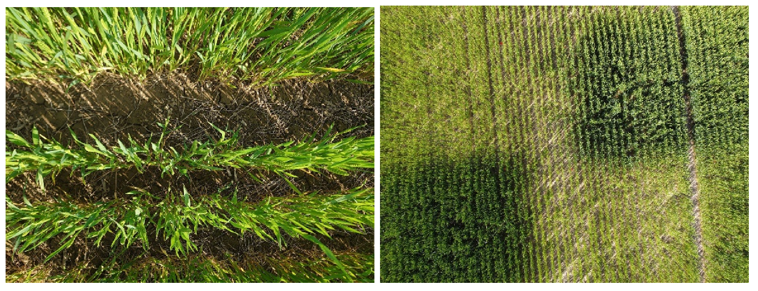
Two types of digital camera images were collected at the canopy scale, via near-ground sensing and UAV-based remote sensing, from these plots during all the wheat growing stages, including Tillering and Stem Extension, Heading and Flowering, and Ripening and Maturity. A Sony Xperia 5 with a 12-megapixel Exmor RS CMOS was used to collect the near-ground images with a focal length of 26 mm. A DJI MAVIC pro with 12.35-megapixel CMOS was selected to capture the images from the air with a focal length of 26 mm. The detailed monitoring schedule is shown in Table 1. Figure 2 shows the sample images. A total of 1449 field near ground images are used in this work. The image size is 4032 × 3024. The UAV flight heights are from 10 m to 30 m. The data are georeferenced by the GPS location provided from a drone and orthorectified by approximate nearest neighbours algorithms. This work is performed in the open-sourced software OpenDroneMap [56]. The detailed parameters are shown in Table 2. Two spatial resolutions of the mosaic images are produced, 0.1 and 0.3 cm, respectively.

3.2. Method

In this work, we have proposed a deep learning based framework to accurately estimate the nitrogen status of wheat from remote sensing datasets. This framework consists of two main parts: the spectral–spatial attention vision transformer (SSVT) and a local-to-global self supervised learning method.

3.2.1. Spectral–Spatial attention Vision Transformer (SSVT)

A transformer network named SSVT is developed to accurately estimate the nitrogen status of wheat, capable of capturing both spatial and spectral features from large UAV-based digital aerial imagery. The proposed conceptual architecture is shown in Figure 3. The design rationale is three-fold:
  • As shown in previous research [11], spectral information plays a vital role in determining nitrogen status at leaf and canopy scales. In this work, the spectral-based attention block is proposed to learn spectral-wise features such as colour information.
  • To learn the spatial information, a spatial interaction block is introduced after the spectral-based attention block.
  • To address the quadratic computing complexity of the ViT, the covariance matrix is used to replace the gram matrix, which can help reduce computational complexity from the quadratic complexity ( O ( n 2 ) ) to linear complexity ( O ( n ) ) where n represents the number of input patches.
The input images are first split into patches and flattened into vectors using a linear projection operation. Then, each vector is regarded as a sequence and fed into the transformer encoders. A class token is added to represent an entire image that can be used for classification. It is actually a vector that is learned during gradient descent. In this work, we add the class token in the last encoder block, which only lets encoders’ attention mechanism perform between images. Each encoder consists of two core components, including (1) spectral–spatial attention block, which consists of spectral-based and spatial interaction blocks, and (2) Multi-Layer Perceptron (MLP).

Spectral–Spatial Attention Block

In this work, to address the spectral and spatial information in the transformer encoder, we proposed a spectral–spatial attention block (this is different from the Multi-Head Self Attention Layer in the original vision transformer network). The spectral–spatial attention block consists of two main parts: Spectral Based Attention (SBA) and Spatial Interaction Block (SIB).

Spectral Based Attention (SBA)

The SBA module adopts an attention mechanism with Query, Key, and Value. In this work, to decrease the computational complexity of the scaled dot-product attention used by a transformer, cross-covariance is proposed to replace the matrix operation in the self-attention function. Given the packed matrix representations of queries Q R n × d , keys K R n × d , and values V R n × d , the cross-covariance attention is given by:
SBA Q , K , V = A X C K , Q V = S o f t M a x K ^ Q ^ τ V
where n denotes the number of patches and d denotes the dimensions of keys (or queries) and values, which means the number of pixels in each patch. A X C K , Q denotes an attention matrix, S o f t M a x is applied in a row-wise manner. Where the attention weights A X C are calculated using a cross-covariance matrix. K ^ Q ^ is the cross-covariance matrix size of d × d . In [57], the author found that controlling the data range in attention strongly enhances the stability of training; here, Q ^ and K ^ denoted the normalized matrices Q and K. The inner products are scaled before the S o f t m a x by the τ which is a learnable parameter that allows for a more precise or consistent distribution of attention weights. The new A X C K , Q operates along the dimensions of input vector d, which denoted the spectral information of the image, rather than along the amount of the patches n. Each output embedding is a convex combination of its corresponding embedding in V’s d features. The computational cost is O ( d 2 n ) which has a linear computational computing complexity of input size. Then, residual connection is used around each module followed by Layer Normalization to generate a deeper model [58]. For instance, each encoder block ( H ) can be written as:
H = LayerNorm SBA x + x

Spatial Interaction Block (SIB)

As SBA only focuses on spectral information, and not the spatial information between patches, a Special Interaction Block (SIB) is therefore introduced to enable explicit communication between patches. The SIB is built with two depth-wise 3 × 3 convolutional layers with Batch Normalization and ReLU non-linearity in between [59]. The output of the SIB can be written as:
S = LayerNorm H + Conv 2 BatchNorm ReLU Conv 1 Conv 1 H

Multilayer Perceptron (MLP)

A multilayer perceptron is a particular case of a feedforward neural network where every layer is a fully connected layer. As is common in transformer models, an MLP is added at the end of each encoder block, which contains two fully connected layers. While the SBA block restricts feature interaction within groups and the SIB cannot allow feature interaction, the MLP allows interaction across all features. The output of MLP (F) can be written as:
F = LayerNorm ( S + F c 2 ( R e L U ( F c 1 ( S ) ) ) )

3.3. Local-to-Global Self-Supervised Learning

In this work, to solve the data-hungry issue of deep learning models training, SSL is used to pretrain the proposed SSVT with unlabelled images. Vision transformer is good at capturing long-range global spatial information. However, it fails to capture the local spatial information of small patches. To address this problem, we have proposed a local-to-global SSL method in which both local and global augmentations are performed to provide both global and local views of the input. The SSL consists of two main steps: the image augmentation and model training.
First, a random high-intensity image augmentation is used on the input images. The image augmentation technique is widely used for supervised and unsupervised training to improve the model’s generalizability. It perturbs and modifies the data and keeps the output invariant, allowing the model to extract the most valuable features for classification. In this work, three types of image enhancement are first used for the input, including random colour augmentation, random rotate/flip, and random erasing. The random colour augmentation consists of brightness/contrast/saturation modifying, colour jittering, Gaussian blur, and solarization. Figure 4 shows the three types of random image augmentation. This image augmentation strategy is also used for the supervised training.
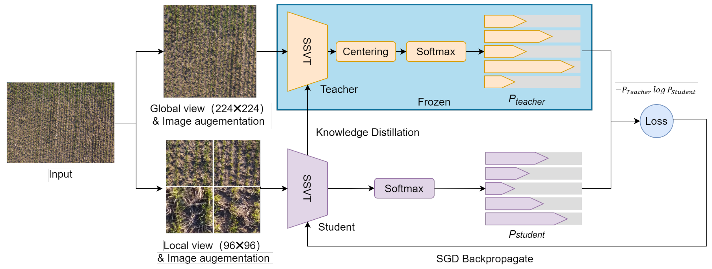
Then, we perform global and local augmentation on the same image to obtain both global and local views. The global views have an image size of 224 × 224. We assume that it contains the global context of the image. The small crops are called local views that have an image size of 96 × 96. It covers less than 50% of the global view. We assume that it contains the local context. Then two views are fed into the SSL network. Figure 5 shows the SSL framework. All local views are passed through the student network, while the global views are passed through the teacher network. It encourages the student network to interpolate context from a small crop and the teacher network to interpolate context from a bigger image.
The SSL network learns through a process called ’self-distillation’ proposed by the paper ‘Be Your Own Teacher’ [60]. There is a teacher and student network both using the proposed model SSVT. They have the same configuration with the same parameters and weights. The teacher is a momentum teacher in that all the weights are frozen and updated by students’ weights ( θ s ) through an exponentially moving average. The update rule for the teacher’s weights ( θ t ) is:
θ t λ θ t + 1 λ θ s
with λ following a cosine schedule from 0.996 to 1 during training. The cross-entropy loss is used to make the two distributions the same, just as in knowledge distillation.
L o s s = P T e a c h e r l o g P S t u d e n t
Centring [53] is used to prevent the model from predicting a uniform distribution along all dimensions or dominated by one dimension regardless of the entry. The teacher’s raw activations ( A t ( x ) ) have their exponentially moving average (c) subtracted from them. The centre c is updated with an exponential moving average. The algorithm is shown in Algorithm 1.
A t ( x ) A t ( x ) c
Algorithm 1 Local-to-Global SSL algorithm
Require:
  • x _ b a t c h : One batch images;
  • T: Teacher Network;
  • S: Student Network;
1:
set T . p a r a m s = S . p a r a m s ;
2:
set T . F r o z e n ( ) # Frozen Teacher’s params;
3:
forxin  x _ b a t c h  do # One batch training
4:
     x 1 = G l o b a l a u g ( x ) # Global view with regular augmentation
5:
     x 2 = L o c a l a u g ( x ) # Local view with regular augmentation
6:
     t 1 , t 2 = T ( x 1 ) , T ( x 2 )
7:
     s 1 , s 2 = S ( x 1 ) , S ( x 2 )
8:
     l o s s = L ( t 1 , s 2 ) / 2 + L ( t 2 , s 1 ) / 2 # L ( a , b ) = a log b
9:
    loss.backward() # Back-propagate
10:
    Update(S.params) # Student params update by SGD
11:
     T . p a r a m s = λ T . p a r a m s + ( 1 λ ) S . p a r a m s # Teacher params update by knowledge distillation
12:
end for

3.4. Model Evaluation

3.4.1. Experimental Design

To evaluate the performance of the proposed SSVT, we have conducted three types of experiments: (1) Performance evaluation of SSVT for automated crop N prediction; (2) Ablation Study; and (3) Evaluation of the generalizability of the proposed model using independent datasets.

Performance Evaluation of SSVT for Automated Crop N Prediction

To evaluate the performance of the proposed SSVT for Crop N prediction, we first train the model based on the configuration (Section 3.4.3) with two different input sizes. The performance of the model including precision, recall and F1-score (Section 3.4.2) for each class and overall accuracy are reported. Then, we compare the proposed SSVT with five state-of-the-art DL models. Two commonly used CNN based architectures, ResNet [61] and EfficientNet [62], with their state-of-the-art versions RegNet [63] and EfficientNetV2 [64] along with ViT are selected for the performance comparison.

Ablation Study

In this case, two ablation studies are set to evaluate: (1) the performance of the proposed SSVT with and without SSL; (2) the impact of the spectral–spatial attention block.

The Performance of the Proposed SSVT with and without SSL

In this work, a local-to-global SSL method is proposed to pretrain the model on the unlabelled image generated from the drone. We evaluate the performance of the proposed SSVT trained from SSL and trained from scratch to show the impact of the SSL on model generalization.

The Impact of the Spectral–Spatial Attention Block

This work proposes the spectral–spatial attention block to replace the self-attention in the original ViT, making the attention module attend over the spectral and spatial information. In this case, we evaluate the effect of the proposed model, compared to the original vision transformer (the ViT-small with a similar number of parameters is selected in this work).

Evaluation of the Generalizability of the Proposed Model Using Independent Drone Datasets

In this case, to evaluate the generalizability of the proposed SSVT model, we have evaluated the trained model on independent datasets. The images are captured from the drone in every growing stage, including Tillering and Stem Extension, Heading and Flowering, and Ripening and Maturity.

3.4.2. Evaluation Metrics

Accuracy, Precision, Recall, F1-score, and the Confusion matrix are selected for the accuracy assessment to evaluate model performance. Accuracy is the most intuitive performance measure, as it is simply a ratio of correctly predicted observations to the total observations. The Precision measures the fraction of true positive detections, and the Recall measures the fraction of correctly identified positives. The F1-score considers both the Precision and the Recall to compute the score. The study establishes the classification matrices which Precision, Recall, and F1-score calculated with the following equations:
Accuracy = TP + TN TP + TN + FP + FN
Precision = TP TP + FP
Recall = TP TP + FN
F 1 -score = Recall × Precision Recall + Precision × 2
where True Positives (TP) are the correctly predicted positive values. True Negatives (TN) are the correctly predicted negative values. False positives and false negatives occur when the actual class contradicts the predicted class. False Positives (FP) mean the predicted class is yes when the actual class is no. False Negatives (FN) mean predicted class in no when actual class is yes.

3.4.3. Experimental Configuration

This work aims to develop a new method for accurately estimating N status in crops (i.e., wheat in this case) based on crop images at the canopy scale. There are four types of N treatments, including High, Medium, Low, and Control, our task is to classify the images into these four categories automatically. Figure 1b shows images collected from different plots with different treatments. We randomly cropped them into 224 × 224 patches for the drone images and generated the unlabelled images for SSL. In this work, 4,800,000 images are generated. The SSL training uses the AdamW optimizer and a batch size of 64, distributed over 3 GPUs (GeForce RTX 2080 Ti). The learning rate is linearly ramped up during the first ten epochs as 1 × 10 3 . After this warmup, we decay the learning rate with a cosine schedule. The weight decay also follows a cosine schedule from 0.04 to 0.4.
The detailed configuration of the proposed SSVT and ViT is shown in Table 3. It has 12 encoder layers. The dimension of keys is 384. To achieve the best performance of the model, we have tested it with two input sizes. As remote sensing data, the larger input covers a larger area and more spatial features can be covered. One input size is 224 × 224 , which is the default input size for most deep learning algorithms. The other is 384 × 384 , which is 1.5 times of the default size.
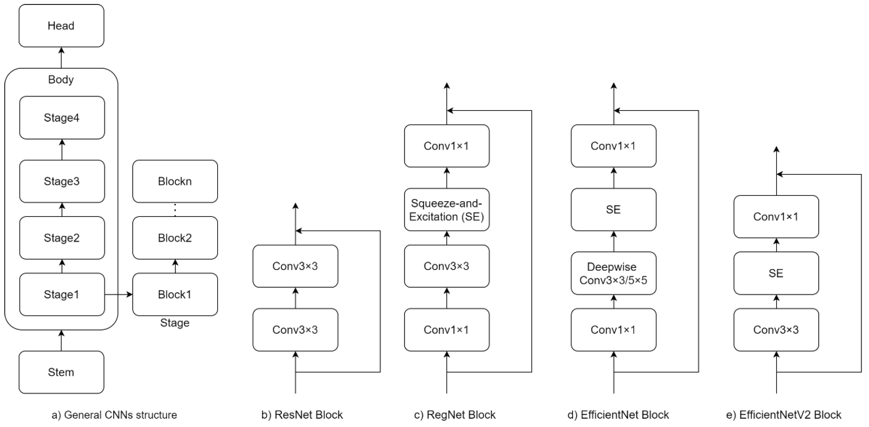
The general network structure of selected models for comparison can be summarized as Figure 6a, which consists of a stem, followed by the body part, and head classifier (average pooling followed by a fully connected layer) that predicts output classes. The body part is composed of four stages that operate at progressively reduced resolution, and each stage consists of a sequence of identical blocks. The identical blocks of each model are shown in Figure 6b–e. For direct comparisons and to isolate benefits resulting from network design, the configuration of the models is based on the trained parameters, in which 20 million parameters are selected as the baseline in this work. Based on this, the ResNet with 50 layers, EfficientNet_B5, RegNetY-4.0G, and EfficientNetv2_small are selected for comparison.
For the supervised training on SSVT and the selected models for comparison. We first transfer the weights learned from SSL training to initialize the model. AdamW optimizer is used for 100 epochs using a cosine decay learning rate scheduler and 20 epochs of linear warm-up. A batch size of 64, a lower initial learning rate of 1 × 10 4 , and a weight decay of 0.05 are used for model training. The augmentation and regularization strategies used in this training to avoid over-fitting include conventional image augmentation mentioned in Section 3.2, random-size cropping, data mix-up [65], and label-smoothing [66] regularization. We used five-fold cross-validation in this study. The dataset is divided into five groups at random, with four groups (80% of dataset) utilised for training and the remaining groups used for testing each time. The average of the accuracies on the testing set over all folds is used to evaluate the classification performance. All models used in this paper are developed using Pytorch 1.6 and the image augmentation are based on the open-sourced image augmentation library Albumentations [67].

4. Result

4.1. Performance Evaluation of SSVT for Automated Crop N Prediction

In this case, we report the performance of the proposed SSVT for automated crop N prediction with two input sizes (Table 4). With the input image size of 224 × 224 , the accuracy of the proposed model reaches 0.962. With the input image size of 384 × 384 , the accuracy of the proposed model reaches 0.965, which is slightly higher. For the rest of the evaluations and comparisons, we select 224 × 224 as the input size.
Meanwhile, we have compared our proposed model with the five most widely used CNN models. The results are shown in Table 5. With the lowest flops and the most parameters, EfficientNet reaches an accuracy of 0.95. The proposed model has intermediate parameters and the highest flops. The performance outperforms other approaches.

4.2. Ablation Study

4.2.1. The Performance of the Proposed SSVT with and without SSL

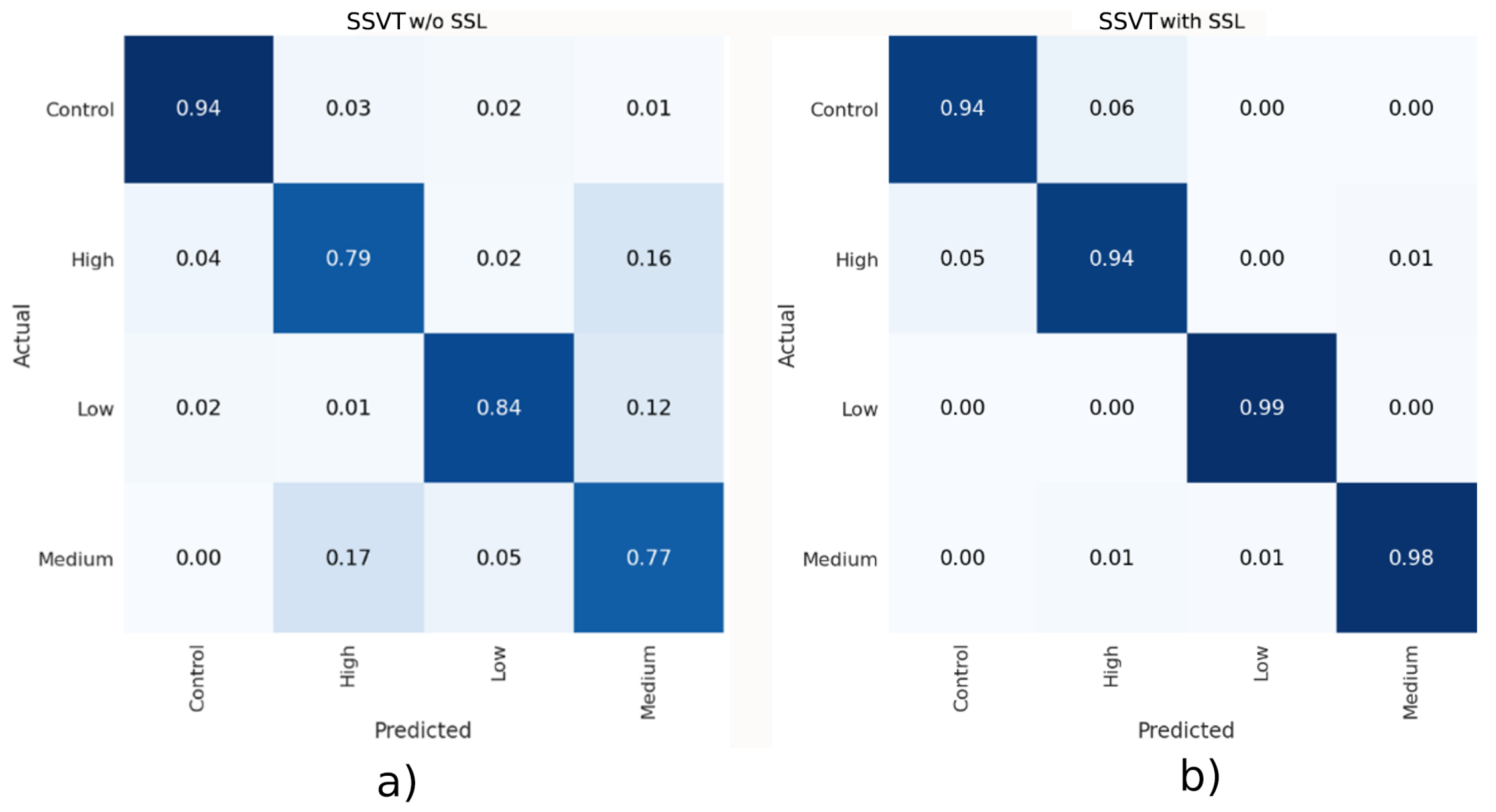
In this case, we train the model with initialized weights based on labelled data. The classification performance of the proposed model without SSL is reported in Table 6 and Figure 7. Without the pretrained weights from SSL, the proposed SSVT cannot converge correctly. The Accuracy of the proposed model is only 0.836. As shown in Figure 7, the model without SSL performs well on N status (Control). However, it performs unsatisfactorily on other statuses, including High, Low, and Medium. Conversely, the model trained with SSL weights performs well on all N statuses.

4.2.2. The Impact of the Spectral–Spatial Attention Block

In this case, to evaluate the effect of the proposed spectral–spatial attention block on vision transformer, we report the model performance of the proposed model and the original ViT. The results are shown in Table 7, demonstrating that our proposed model with spectral–spatial attention block has better classification performance for crop N status estimation than that of ViT.

4.3. Evaluation of the Generalizability of the Proposed Model Using Independent Datasets

To evaluate the generalizability of the proposed SSVT model, we evaluate the trained model on independent drone datasets captured at every growing stage, including Tillering and Stem Extension, Heading and Flowering, and Ripening and Maturity. The performance of the trained model on each growing stage are reported in Figure 8.
Compared to the model’s accuracy based on the ground field data, the accuracy of proposed model on independent drone data is slightly decreased. The accuracy in Tillering and Stem Extension, Heading and Flowering, and Ripening and Maturity is 0.939, 0.926, and 0.933, respectively. However, the performance of ResNet on independent drones dropped significantly. Compared to its accuracy on ground field data, it dropped by 0.07, 0.049, and 0.033, respectively, in each growing stage. Figure 9 shows the N status estimation result on drone images captured at the early growing stage (Tillering and Stem Extension). In the early stages of crop growth, all characteristics are not prominent. The estimated result of ResNet shows many misclassifications. The result of our proposed model is more precise and more accurate. The result shows the good generalizability of our proposed model.

5. Discussion

In this work, we propose a new deep learning-based method for accurately estimating the nitrogen status of wheat using images from UAV imagery named SSVT. Three experiments are designed to evaluate the performance of the model. Our discussions are based around the experiment results.

5.1. Performance of SSVT for Automated Crop N Prediction

In the first experiment, we have evaluated the accuracy of the model and compared it with the existing state-of-the-art deep learning models including ResNet, its latest version RegNet, and EfficientNet v1 and v2. The results demonstrate that our proposed model achieves an overall accuracy of 0.962. Under the similar parameters (20–30 millions), the classification accuracy of the proposed method outperforms the comparative structures. In general, the performance of model estimation on the nitrogen status of crops using RGB digital images might be affected by several factors, such as inconsistent image brightness and white balance in multiple observations, the shadow of crops and the soil background [68]. To avoid the effect of shadows on images, all the data in this work are taken at 11–12 AM to reduce the shadow of the plants and ensure sufficient light conditions. Moreover, we have performed high-intensity image colour augmentation for model training, including brightness/contrast/saturation, modifying, colour jittering, and solarization (Figure 4). This is considered effective in improving the generalisability and robustness of the model [69], thus allowing it to maintain performance under different lighting conditions.
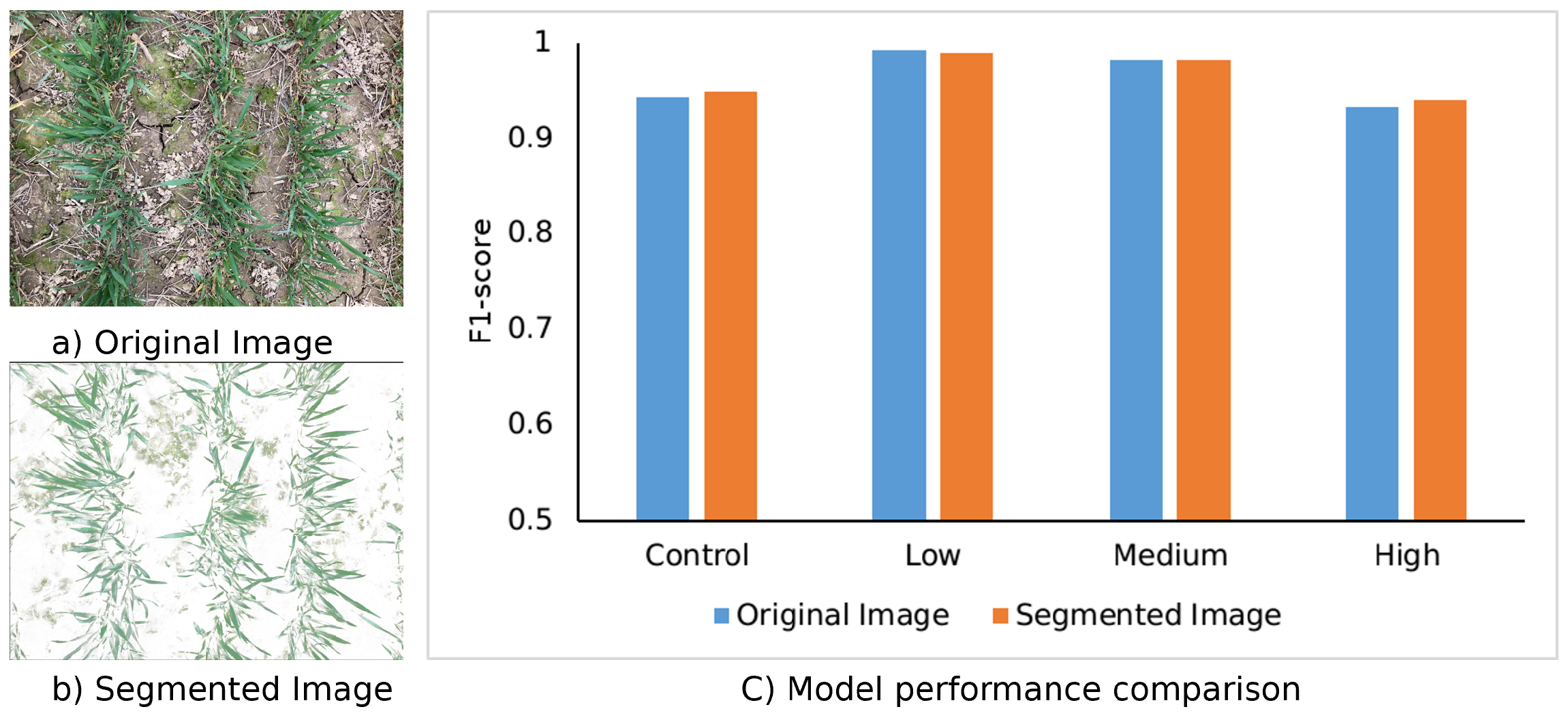
For the impact of soil background, the typical method to remove the effect is to segment the soil from the image, as shown in Figure 10a,b. However, automatically identifying and segmenting crops from soil correctly in the high-resolution image is one of the most challenging problems in precision agriculture [70,71]. In this work, a simple comparison experiment is performed to evaluate the performance using original and segmented images. The crop is segmented by a dynamic colour threshold through manual visual interpretation on each image. The F1-scores for each class of the models’ performance are shown in Figure 10c. The model using the segmented images does not improve the model’s performance, and the results demonstrate that the proposed model has the ability to remove the effects of background from complex images.
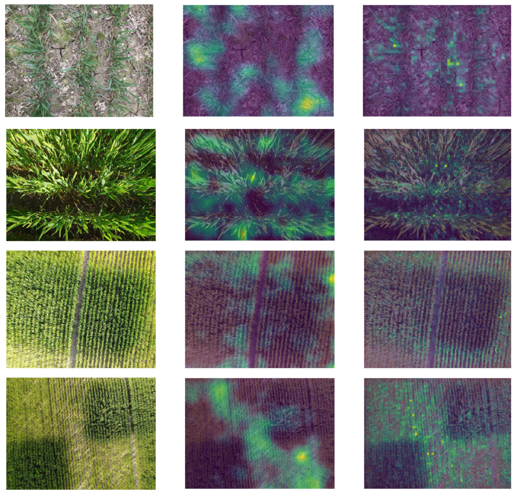
To deeply investigate the reasons for the result to remove the background of our proposed SSVT, we visualize the attention map from the last block of the trained model to explain the decision-making area. The attention maps are shown in Figure 11. The middle column is the attention map of the ResNet model, and the right column is the map of the proposed SSVT. The images in the first two lines are captured in the field, and the attention maps show that the two models highlight the plant area from the first two lines. This result can explain why the soil background does not affect the deep learning-based model’s performance on crop N status estimation. The last two lines show the attention area on UAV images. The attention map of the proposed SSVT distinguishes well between regions with different N statuses. The attention map of ResNet also distinguishes between different regions, but not as clearly as the proposed SSVT. This leads to the higher accuracy of our proposed SSVT on independent drone data. Our third experiment evaluates the generalizability of the proposed model using independent UAV datasets. The results demonstrate that our proposed model outperforms the existing models in every growing stage.
It is unfair to perform the direct comparison between existing wheat nitrogen predict methods due to the use of different datasets and analysis methods (spectral analysis). In this case, we have only indirectly compared our model with five existing methods [37,72,73,74,75]. The results are shown in Table 8, showing that the proposed SSVT outperforms other approaches. This result may be due to two possible reasons. Firstly, most existing methods used only the spectral information, whereas our method utilizes both spectral and spatial features, enhancing the data usage. Secondly, our method uses a deep network to extract features from all the data, which is considered to be superior to traditional handcrafted features.

5.2. Prospects and Future Work

In this work, there are three main innovations of the proposed framework including (1) the SSL for model training with unlabelled datasets; (2) a novel spectral–spatial attention-based vision transformer network; and (3) the computational complexity optimization on transformer network.
The first is the SSL for model training with unlabelled datasets. In the second experiment, we evaluate the impact of the SSL. The result shows that the proposed model does not converge well when we train the model from init weight. The accuracy is only 0.836. However, when we trained the model with the weights from SSL, the model converged well and achieved the best performance. Figure 12a shows the loss trend in SSL, which shows the model converges correctly. It indicates that the model can extract the similar features from the different views (‘local’ and ‘global’ views) of the same image. In Figure 12b, we visualize the features extracted from the labelled data based on the model trained with SSL by the t-SNE (van der Maaten Hinton, 2008). Although there are points that remain integrated with other points belonging to other classes, various clusters are easily recognized by different N statuses. This result explains why SSL can help the model train without labelled data. The proposed SSL is generic, which can be applied to other applications with limited labelled datasets. Particularly, remote sensing applications often have large amounts of data but lack annotation. We believe our approach will significantly contribute to the remote sensing field through SSL from unlabelled data.
The second innovation is that the proposed SSVT is capable of simultaneously capturing both spatial and spectral based features for accurate nitrogen diagnosis. In the experiment, we evaluate the performance of the proposed method compared to the existing vision transformer networks, focusing on spatial features only. The results indicate that, by adding the SBA and SIB we proposed, our model achieves better accuracy. The SSVT is also a generic network. In this paper, we have used it on RGB datasets and achieved satisfactory results. We believe it can be applied to multi- to hyper-spectral datasets and we will deliver this work in the future.
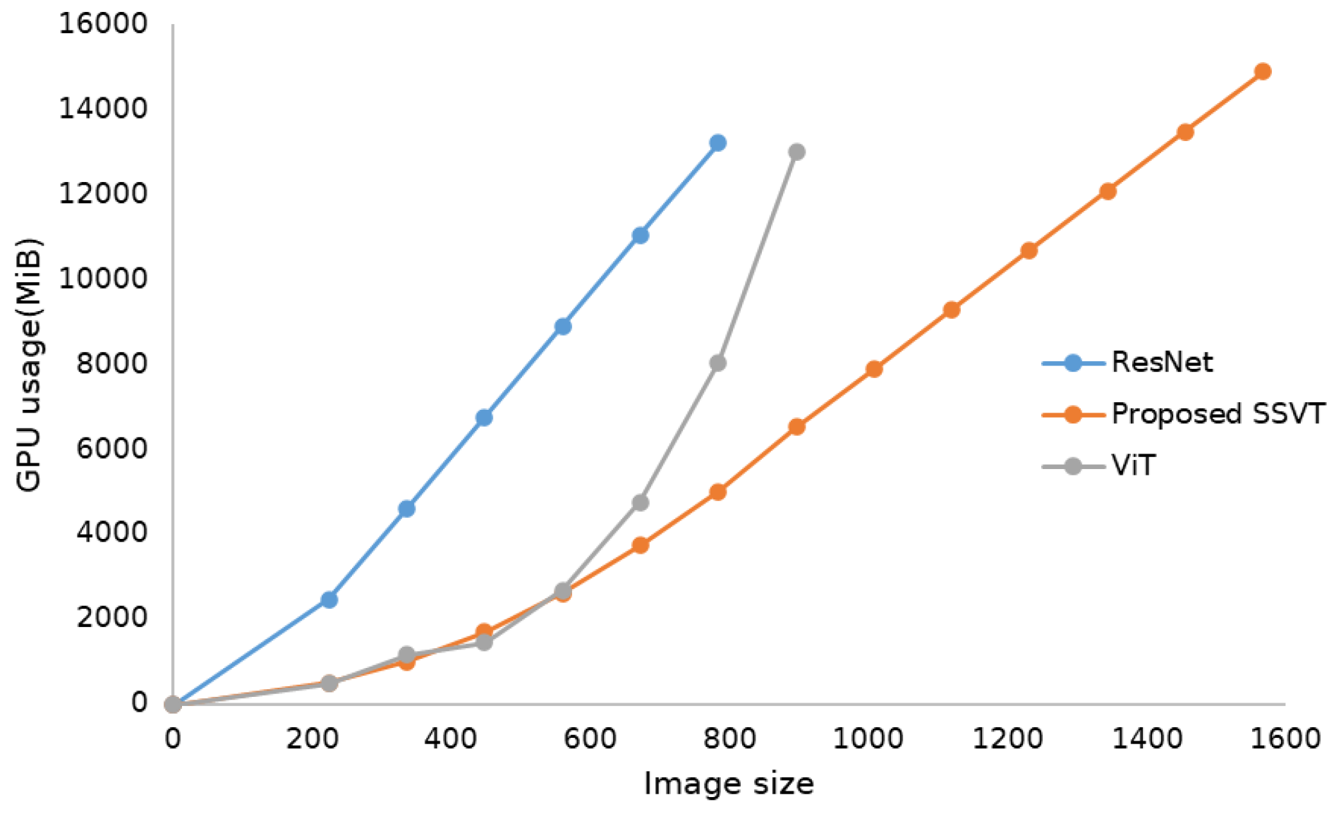
The third innovation is the computational complexity optimization. The deep learning-based methods typically have millions of parameters, resulting in massive computational consumption. The original ViT has quadratic computational complexity to the image size due to the self-attention operation, which limits its usage on large images. In this work, the cross-covariance matrix is used to replace the gram matrix operation in the attention module. It changes the complexity of the transformer layer from quadratic to linear, which makes it possible for the model to handle large size images. We calculate and report the GPU usage of three models with increased input image size. We start from the commonly used size of 224 × 224 and then gradually and linearly increase the size of the input image (336, 448, 560, ……). The most widely used CNN model, ResNet with 50 layers, and the original ViT, are selected for comparison. The inference GPU memory usage of the ResNet, the original VIT, and the proposed SSVT are shown in Figure 13. Our proposed SSVT has linear computational complexity with the size of the input image, which makes it possible to scale to a much larger image size (1600 × 1600 with 16GB GPU memory and 1344 × 1344 with 12 GB GPU memory). The original VIT has quadratic computational complexity to the image size, which can only handle images with a size of 896 × 896 in 16 GB GPU memory and 784 × 784 in 12 GB GPU memory. Meanwhile, the proposed model has better computational efficiency and utilization than the CNN based model (ResNet).
In this paper, we proposed a novel SSVT for accurately estimating the nitrogen status of wheat. The fertiliser application rates were chosen to be realistic based on low to high rates used by extensive and intensive farmers. This was so as to include the ranges of possible values which could be observed on different farms. Additionally, fertiliser application is not uniform, particularly when it is applied as a solid. This leads to hotspots and variation within and between fields, even when fertiliser has been applied at the same rate. However, it should be noted that further work is needed to determine whether our approach will perform equally well if the ranges of values within a field is diminished, our approach was able to distinguish between crops growing in treatments which differed by 80 kg ha yr 1 .
Our approach provides farmers with a higher frequency and resolution of data than is currently possible. Typically, farmers rely on a small number of soil samples taken prior to the growing season to calculate optimal application rates for a whole field or farm. This is achieved by comparing soil sample values with industry standards (e.g., RB209 [76]). Using our higher resolution approach, data that has been gathered can be compared with industry benchmarks to inform farmer decision making on N fertiliser application rates and locations within the same growing season and within the same field. This may allow farmers to only apply fertiliser where and when it is needed. Future work could combine crop yield and quality data with N status data gathered using our approach to review these guidelines and advise on locally appropriate optimal fertiliser rates.
Although we have conducted a lot of data augmentation on the model training to improve the model’s generalizability, and the model obtained satisfactory results on independent data in different growing stages, this is not fully representative of the actual conditions. We will continuously collect data covering different conditions across different time windows, areas, and crop types to evaluate the proposed model.

6. Conclusions

We have proposed a novel spectral–spatial attention-based vision transformer (SSVT) for accurately estimating the nitrogen status of wheat using images from UAV imagery. The model framework proposes a spectral–spatial attention block consists of SBA and SIB, which can simultaneously learn both spatial and spectral features for accurate crop N estimation. The proposed model has been compared with state-of-the-art methods as well as being evaluated on both testing and independent datasets. The experimental results show competitive advantages over the existing works in terms of accuracy and computing performance, and model generalizability. Moreover, as model training requires massive labelled data, which is time consuming and costly. A local-to-global self-supervised learning has been introduced to pre-train the model with unlabelled data. We believe this approach will significantly contribute to the remote sensing field through self-supervised learning from unlabelled data. Meanwhile, the cross-covariance matrix is used to reduce the computational complexity of the model from quadratic to linear, which allows the proposed models to operate on a larger area. As a generic method, in the future, we will extend it to other data, especially multi- to hyper-spectral data to take advantage of its ability in both spectral and spatial feature learning.

Author Contributions

Conceptualization, all authors; Methodology, X.Z. and L.H.; Data acquisition and processing, A.H., L.L., M.A.L. and A.K.; Software, X.Z. and T.S.; Analysis, X.Z., L.H. and M.A.L.; Writing—original draft preparation, X.Z.; Writing—review and editing, X.Z., M.A.L. and L.H.; Project administration, L.H.; Funding acquisition, L.H. All authors have read and agreed to the published version of the manuscript.

Funding

The work reported in this paper has formed part of the N2Vision project funded by UKRI-ISCF-TFP (Grant No. 134063).

Institutional Review Board Statement

Not applicable.

Informed Consent Statement

Not applicable.

Acknowledgments

We thank the anonymous reviewers for reviewing the manuscript and providing comments to improve the manuscript.

Conflicts of Interest

The authors declare no conflict of interest.

References

  1. FAO. World Fertilizer Trends and Outlook to 2020: Summary Report; FAO: Rome, Italy, 2017. [Google Scholar]
  2. Good, A. Toward nitrogen-fixing plants. Science 2018, 359, 869–870. [Google Scholar] [CrossRef]
  3. Berger, K.; Verrelst, J.; Féret, J.B.; Wang, Z.; Wocher, M.; Strathmann, M.; Danner, M.; Mauser, W.; Hank, T. Crop nitrogen monitoring: Recent progress and principal developments in the context of imaging spectroscopy missions. Remote Sens. Environ. 2020, 242, 111758. [Google Scholar] [CrossRef]
  4. Wang, D.; Xu, Z.; Zhao, J.; Wang, Y.; Yu, Z. Excessive nitrogen application decreases grain yield and increases nitrogen loss in a wheat–soil system. Acta Agric. Scand. Sect. B-Soil Plant Sci. 2011, 61, 681–692. [Google Scholar] [CrossRef]
  5. Knoema. Wheat Area Harvested. 2021. Available online: https://knoema.com//atlas/topics/Agriculture/Crops-Production-Area-Harvested/Wheat-area-harvested (accessed on 8 August 2021).
  6. Benitez Ramirez, M. Monitoring Nitrogen Levels in the Cotton Canopy Using Real-Time Active-Illumination Spectral Sensing. Master’s Thesis, University of Tennessee, Knoxville, TN, USA, 2010. [Google Scholar]
  7. Wang, J.; Shen, C.; Liu, N.; Jin, X.; Fan, X.; Dong, C.; Xu, Y. Non-destructive evaluation of the leaf nitrogen concentration by in-field visible/near-infrared spectroscopy in pear orchards. Sensors 2017, 17, 538. [Google Scholar] [CrossRef] [Green Version]
  8. Imani, M.; Ghassemian, H. An overview on spectral and spatial information fusion for hyperspectral image classification: Current trends and challenges. Inf. Fusion 2020, 59, 59–83. [Google Scholar] [CrossRef]
  9. Johnson, D.M. An assessment of pre-and within-season remotely sensed variables for forecasting corn and soybean yields in the United States. Remote Sens. Environ. 2014, 141, 116–128. [Google Scholar] [CrossRef]
  10. Fitzgerald, G.; Rodriguez, D.; O’Leary, G. Measuring and predicting canopy nitrogen nutrition in wheat using a spectral index—The canopy chlorophyll content index (CCCI). Field Crops Res. 2010, 116, 318–324. [Google Scholar] [CrossRef]
  11. Chlingaryan, A.; Sukkarieh, S.; Whelan, B. Machine learning approaches for crop yield prediction and nitrogen status estimation in precision agriculture: A review. Comput. Electron. Agric. 2018, 151, 61–69. [Google Scholar] [CrossRef]
  12. Jordan, M.I.; Mitchell, T.M. Machine learning: Trends, perspectives, and prospects. Science 2015, 349, 255–260. [Google Scholar] [CrossRef]
  13. Shi, P.; Wang, Y.; Xu, J.; Zhao, Y.; Yang, B.; Yuan, Z.; Sun, Q. Rice nitrogen nutrition estimation with RGB images and machine learning methods. Comput. Electron. Agric. 2021, 180, 105860. [Google Scholar] [CrossRef]
  14. Qiu, Z.; Ma, F.; Li, Z.; Xu, X.; Ge, H.; Du, C. Estimation of nitrogen nutrition index in rice from UAV RGB images coupled with machine learning algorithms. Comput. Electron. Agric. 2021, 189, 106421. [Google Scholar] [CrossRef]
  15. Zhang, X.; Han, L.; Han, L.; Zhu, L. How well do deep learning-based methods for land cover classification and object detection perform on high resolution remote sensing imagery? Remote Sens. 2020, 12, 417. [Google Scholar] [CrossRef] [Green Version]
  16. Roth, L.; Streit, B. Predicting cover crop biomass by lightweight UAS-based RGB and NIR photography: An applied photogrammetric approach. Precis. Agric. 2018, 19, 93–114. [Google Scholar] [CrossRef] [Green Version]
  17. Alom, M.Z.; Hasan, M.; Yakopcic, C.; Taha, T.M.; Asari, V.K. Improved inception-residual convolutional neural network for object recognition. Neural Comput. Appl. 2018. [Google Scholar] [CrossRef] [Green Version]
  18. Nanni, L.; Ghidoni, S.; Brahnam, S. Handcrafted vs. non-handcrafted features for computer vision classification. Pattern Recognit. 2017, 71, 158–172. [Google Scholar] [CrossRef]
  19. Lewis, K.P.; Espineli, J.D. Classification And Detection of Nutritional Deficiencies in Coffee Plants Using Image Processing And Convolutional Neural Network (CNN). Int. J. Sci. Technol. Res. 2020, 9, 6. [Google Scholar]
  20. Sethy, P.K.; Barpanda, N.K.; Rath, A.K.; Behera, S.K. Nitrogen Deficiency Prediction of Rice Crop Based on Convolutional Neural Network. J. Ambient. Intell. Humaniz. Comput. 2020, 11, 5703–5711. [Google Scholar] [CrossRef]
  21. Tran, T.T.; Choi, J.W.; Le, T.T.H.; Kim, J.W. A Comparative Study of Deep CNN in Forecasting and Classifying the Macronutrient Deficiencies on Development of Tomato Plant. Appl. Sci. 2019, 9, 1601. [Google Scholar] [CrossRef] [Green Version]
  22. Wolf, T.; Debut, L.; Sanh, V.; Chaumond, J.; Delangue, C.; Moi, A.; Cistac, P.; Rault, T.; Louf, R.; Funtowicz, M.; et al. Transformers: State-of-the-Art Natural Language Processing. In Proceedings of the 2020 Conference on Empirical Methods in Natural Language Processing: System Demonstrations, Online, 16–20 November 2020; Association for Computational Linguistic, 2020; pp. 38–45. Available online: https://aclanthology.org/2020.emnlp-demos.6/ (accessed on 12 May 2021).
  23. Scharf, P.; Schmidt, J.; Kitchen, N.; Sudduth, K.; Hong, S.; Lory, J.; Davis, J. Remote sensing for nitrogen management. J. Soil Water Conserv. 2002, 57, 518–524. [Google Scholar]
  24. Hunt, E.R., Jr.; Doraiswamy, P.C.; McMurtrey, J.E.; Daughtry, C.S.; Perry, E.M.; Akhmedov, B. A visible band index for remote sensing leaf chlorophyll content at the canopy scale. Int. J. Appl. Earth Obs. Geoinf. 2013, 21, 103–112. [Google Scholar] [CrossRef] [Green Version]
  25. Solovchenko, A.; Merzlyak, M. Screening of visible and UV radiation as a photoprotective mechanism in plants. Russ. J. Plant Physiol. 2008, 55, 719–737. [Google Scholar] [CrossRef]
  26. Yang, W.H.; Peng, S.; Huang, J.; Sanico, A.L.; Buresh, R.J.; Witt, C. Using leaf color charts to estimate leaf nitrogen status of rice. Agron. J. 2003, 95, 212–217. [Google Scholar] [CrossRef]
  27. Baret, F.; Hagolle, O.; Geiger, B.; Bicheron, P.; Miras, B.; Huc, M.; Berthelot, B.; Niño, F.; Weiss, M.; Samain, O.; et al. LAI, fAPAR and fCover CYCLOPES global products derived from VEGETATION: Part 1: Principles of the algorithm. Remote Sens. Environ. 2007, 110, 275–286. [Google Scholar] [CrossRef] [Green Version]
  28. Hank, T.B.; Berger, K.; Bach, H.; Clevers, J.G.; Gitelson, A.; Zarco-Tejada, P.; Mauser, W. Spaceborne imaging spectroscopy for sustainable agriculture: Contributions and challenges. Surv. Geophys. 2019, 40, 515–551. [Google Scholar] [CrossRef] [Green Version]
  29. Lu, B.; He, Y. Evaluating empirical regression, machine learning, and radiative transfer modelling for estimating vegetation chlorophyll content using bi-seasonal hyperspectral images. Remote Sens. 2019, 11, 1979. [Google Scholar] [CrossRef] [Green Version]
  30. Wocher, M.; Berger, K.; Danner, M.; Mauser, W.; Hank, T. RTM-based dynamic absorption integrals for the retrieval of biochemical vegetation traits. Int. J. Appl. Earth Obs. Geoinf. 2020, 93, 102219. [Google Scholar] [CrossRef]
  31. Verhoef, W. Light scattering by leaf layers with application to canopy reflectance modeling: The SAIL model. Remote Sens. Environ. 1984, 16, 125–141. [Google Scholar] [CrossRef] [Green Version]
  32. Wang, Z.; Skidmore, A.K.; Darvishzadeh, R.; Heiden, U.; Heurich, M.; Wang, T. Leaf nitrogen content indirectly estimated by leaf traits derived from the PROSPECT model. IEEE J. Sel. Top. Appl. Earth Obs. Remote Sens. 2015, 8, 3172–3182. [Google Scholar] [CrossRef]
  33. Padilla, F.M.; Gallardo, M.; Peña-Fleitas, M.T.; De Souza, R.; Thompson, R.B. Proximal optical sensors for nitrogen management of vegetable crops: A review. Sensors 2018, 18, 2083. [Google Scholar] [CrossRef] [PubMed] [Green Version]
  34. Clevers, J.G.; Gitelson, A.A. Remote estimation of crop and grass chlorophyll and nitrogen content using red-edge bands on Sentinel-2 and-3. Int. J. Appl. Earth Obs. Geoinf. 2013, 23, 344–351. [Google Scholar] [CrossRef]
  35. Afandi, S.D.; Herdiyeni, Y.; Prasetyo, L.B.; Hasbi, W.; Arai, K.; Okumura, H. Nitrogen content estimation of rice crop based on near infrared (NIR) reflectance using artificial neural network (ANN). Procedia Environ. Sci. 2016, 33, 63–69. [Google Scholar] [CrossRef] [Green Version]
  36. Pagola, M.; Ortiz, R.; Irigoyen, I.; Bustince, H.; Barrenechea, E.; Aparicio-Tejo, P.; Lamsfus, C.; Lasa, B. New method to assess barley nitrogen nutrition status based on image colour analysis: Comparison with SPAD-502. Comput. Electron. Agric. 2009, 65, 213–218. [Google Scholar] [CrossRef]
  37. Zha, H.; Miao, Y.; Wang, T.; Li, Y.; Zhang, J.; Sun, W.; Feng, Z.; Kusnierek, K. Improving unmanned aerial vehicle remote sensing-based rice nitrogen nutrition index prediction with machine learning. Remote Sens. 2020, 12, 215. [Google Scholar] [CrossRef] [Green Version]
  38. Mehra, L.K.; Cowger, C.; Gross, K.; Ojiambo, P.S. Predicting pre-planting risk of Stagonospora nodorum blotch in winter wheat using machine learning models. Front. Plant Sci. 2016, 7, 390. [Google Scholar] [CrossRef]
  39. Lee, K.J.; Lee, B.W. Estimating canopy cover from color digital camera image of rice field. J. Crop Sci. Biotechnol. 2011, 14, 151–155. [Google Scholar] [CrossRef]
  40. Li, Y.; Chen, D.; Walker, C.N.; Angus, J.F. Estimating the nitrogen status of crops using a digital camera. Field Crops Res. 2010, 118, 221–227. [Google Scholar] [CrossRef]
  41. Zhao, B.; Zhang, Y.; Duan, A.; Liu, Z.; Xiao, J.; Liu, Z.; Qin, A.; Ning, D.; Li, S.; Ata-Ul-Karim, S.T. Estimating the Growth Indices and Nitrogen Status Based on Color Digital Image Analysis During Early Growth Period of Winter Wheat. Front. Plant Sci. 2021, 12, 502. [Google Scholar] [CrossRef]
  42. Azimi, S.; Kaur, T.; Gandhi, T.K. A deep learning approach to measure stress level in plants due to Nitrogen deficiency. Measurement 2021, 173, 108650. [Google Scholar] [CrossRef]
  43. Lee, S.H.; Chan, C.S.; Mayo, S.J.; Remagnino, P. How deep learning extracts and learns leaf features for plant classification. Pattern Recognit. 2017, 71, 1–13. [Google Scholar] [CrossRef] [Green Version]
  44. Islam, M.A.; Jia, S.; Bruce, N.D.B. How Much Position Information Do Convolutional Neural Networks Encode? arXiv 2020, arXiv:2001.08248. [Google Scholar]
  45. Vaswani, A.; Shazeer, N.; Parmar, N.; Uszkoreit, J.; Jones, L.; Gomez, A.N.; Kaiser, L.; Polosukhin, I. Attention Is All You Need. arXiv 2017, arXiv:1706.03762. [Google Scholar]
  46. Dong, Y.; Cordonnier, J.B.; Loukas, A. Attention is Not All You Need: Pure Attention Loses Rank Doubly Exponentially with Depth. arXiv 2021, arXiv:2103.03404. [Google Scholar]
  47. Touvron, H.; Cord, M.; Douze, M.; Massa, F.; Sablayrolles, A.; Jégou, H. Training data-efficient image transformers & distillation through attention. arXiv 2021, arXiv:2012.12877. [Google Scholar]
  48. Liu, X.; Zhang, F.; Hou, Z.; Mian, L.; Wang, Z.; Zhang, J.; Tang, J. Self-supervised learning: Generative or contrastive. IEEE Trans. Knowl. Data Eng. 2021, 1. [Google Scholar] [CrossRef]
  49. Goodfellow, I.J.; Pouget-Abadie, J.; Mirza, M.; Xu, B.; Warde-Farley, D.; Ozair, S.; Courville, A.; Bengio, Y. Generative Adversarial Networks. arXiv 2014, arXiv:1406.2661. [Google Scholar] [CrossRef]
  50. Hadsell, R.; Chopra, S.; LeCun, Y. Dimensionality Reduction by Learning an Invariant Mapping. In Proceedings of the 2006 IEEE Computer Society Conference on Computer Vision and Pattern Recognition (CVPR’06), New York, NY, USA, 17–22 June 2006; 2006; Volume 2, pp. 1735–1742. [Google Scholar]
  51. Bromley, J.; Bentz, J.W.; Bottou, L.; Guyon, I.; LeCun, Y.; Moore, C.; Säckinger, E.; Shah, R. Signature verification using a “siamese” time delay neural network. Int. J. Pattern Recognit. Artif. Intell. 1993, 7, 669–688. [Google Scholar] [CrossRef] [Green Version]
  52. Grill, J.B.; Strub, F.; Altché, F.; Tallec, C.; Richemond, P.H.; Buchatskaya, E.; Doersch, C.; Pires, B.A.; Guo, Z.D.; Azar, M.G.; et al. Bootstrap your own latent: A new approach to self-supervised Learning. arXiv 2020, arXiv:2006.07733. [Google Scholar]
  53. Caron, M.; Misra, I.; Mairal, J.; Goyal, P.; Bojanowski, P.; Joulin, A. Unsupervised Learning of Visual Features by Contrasting Cluster Assignments. arXiv 2021, arXiv:2006.09882. [Google Scholar]
  54. He, K.; Fan, H.; Wu, Y.; Xie, S.; Girshick, R. Momentum Contrast for Unsupervised Visual Representation Learning. In Proceedings of the IEEE/CVF Conference on Computer Vision and Pattern Recognition (CVPR 2020), Seattle, WA, USA, 14–19 June 2020; pp. 9729–9738. [Google Scholar]
  55. Chen, T.; Kornblith, S.; Norouzi, M.; Hinton, G. A Simple Framework for Contrastive Learning of Visual Representations. arXiv 2020, arXiv:2002.05709. [Google Scholar]
  56. OpenDroneMap/ODM. A Command Line Toolkit to Generate Maps, Point Clouds, 3D Models and DEMs from Drone, Balloon or Kite Images. 2020. Available online: https://github.com/OpenDroneMap/ODM (accessed on 26 January 2022).
  57. El-Nouby, A.; Touvron, H.; Caron, M.; Bojanowski, P.; Douze, M.; Joulin, A.; Laptev, I.; Neverova, N.; Synnaeve, G.; Verbeek, J.; et al. XCiT: Cross-Covariance Image Transformers. arXiv 2021, arXiv:2106.09681. [Google Scholar]
  58. Ba, J.L.; Kiros, J.R.; Hinton, G.E. Layer Normalization. arXiv 2016, arXiv:1607.06450. [Google Scholar]
  59. Howard, A.G.; Zhu, M.; Chen, B.; Kalenichenko, D.; Wang, W.; Weyand, T.; Andreetto, M.; Adam, H. MobileNets: Efficient Convolutional Neural Networks for Mobile Vision Applications. arXiv 2017, arXiv:1704.04861. [Google Scholar]
  60. Zhang, L.; Song, J.; Gao, A.; Chen, J.; Bao, C.; Ma, K. Be Your Own Teacher: Improve the Performance of Convolutional Neural Networks via Self Distillation. In Proceedings of the 2019 IEEE/CVF International Conference on Computer Vision (ICCV), Seoul, Korea, 27–28 October 2019; pp. 3712–3721. [Google Scholar]
  61. He, K.; Zhang, X.; Ren, S.; Sun, J. Deep residual learning for image recognition. In Proceedings of the IEEE Conference on Computer Vision and Pattern Recognition, Las Vegas, NV, USA, 26 June–1 July 2016; pp. 770–778. [Google Scholar]
  62. Tan, M.; Le, Q. Efficientnet: Rethinking model scaling for convolutional neural networks. In Proceedings of the International Conference on Machine Learning (PMLR), Long Beach, CA, USA, 9–15 June 2019; pp. 6105–6114. [Google Scholar]
  63. Radosavovic, I.; Kosaraju, R.P.; Girshick, R.; He, K.; Dollár, P. Designing Network Design Spaces. arXiv 2020, arXiv:2003.13678. [Google Scholar]
  64. Tan, M.; Le, Q.V. EfficientNetV2: Smaller Models and Faster Training. arXiv 2021, arXiv:2104.00298. [Google Scholar]
  65. Zhang, H.; Cisse, M.; Dauphin, Y.N.; Lopez-Paz, D. mixup: Beyond empirical risk minimization. arXiv 2017, arXiv:1710.09412. [Google Scholar]
  66. Müller, R.; Kornblith, S.; Hinton, G. When does label smoothing help? arXiv 2019, arXiv:1906.02629. [Google Scholar]
  67. Buslaev, A.; Iglovikov, V.I.; Khvedchenya, E.; Parinov, A.; Druzhinin, M.; Kalinin, A.A. Albumentations: Fast and Flexible Image Augmentations. Information 2020, 11, 125. [Google Scholar] [CrossRef] [Green Version]
  68. Putra, B.T.W.; Soni, P. Improving nitrogen assessment with an RGB camera across uncertain natural light from above-canopy measurements. Precis. Agric. 2020, 21, 147–159. [Google Scholar] [CrossRef]
  69. Shorten, C.; Khoshgoftaar, T.M. A survey on image data augmentation for deep learning. J. Big Data 2019, 6, 60. [Google Scholar] [CrossRef]
  70. Hernández-Hernández, J.L.; García-Mateos, G.; González-Esquiva, J.; Escarabajal-Henarejos, D.; Ruiz-Canales, A.; Molina-Martínez, J.M. Optimal color space selection method for plant/soil segmentation in agriculture. Comput. Electron. Agric. 2016, 122, 124–132. [Google Scholar] [CrossRef]
  71. Dyson, J.; Mancini, A.; Frontoni, E.; Zingaretti, P. Deep learning for soil and crop segmentation from remotely sensed data. Remote Sens. 2019, 11, 1859. [Google Scholar] [CrossRef] [Green Version]
  72. Zhang, H.Y.; Ren, X.X.; Zhou, Y.; Wu, Y.P.; He, L.; Heng, Y.R.; Feng, W.; Wang, C.Y. Remotely assessing photosynthetic nitrogen use efficiency with in situ hyperspectral remote sensing in winter wheat. Eur. J. Agron. 2018, 101, 90–100. [Google Scholar] [CrossRef]
  73. Liu, H.; Zhu, H.; Li, Z.; Yang, G. Quantitative analysis and hyperspectral remote sensing of the nitrogen nutrition index in winter wheat. Int. J. Remote Sens. 2020, 41, 858–881. [Google Scholar] [CrossRef]
  74. Cui, R.; Liu, Y.; Fu, J. Estimation of winter wheat leaf nitrogen accumulation using machine learning algorithm and visible spectral. Guang Pu Xue Yu Guang Pu Fen Xi = Guang Pu 2016, 36, 1837–1842. [Google Scholar] [PubMed]
  75. Shah, S.H.; Angel, Y.; Houborg, R.; Ali, S.; McCabe, M.F. A random forest machine learning approach for the retrieval of leaf chlorophyll content in wheat. Remote Sens. 2019, 11, 920. [Google Scholar] [CrossRef] [Green Version]
  76. AHDB. Nutrient Management Guide (RB209)|AHDB. 2021. Available online: https://ahdb.org.uk/nutrient-management-guide-rb209 (accessed on 26 January 2022).
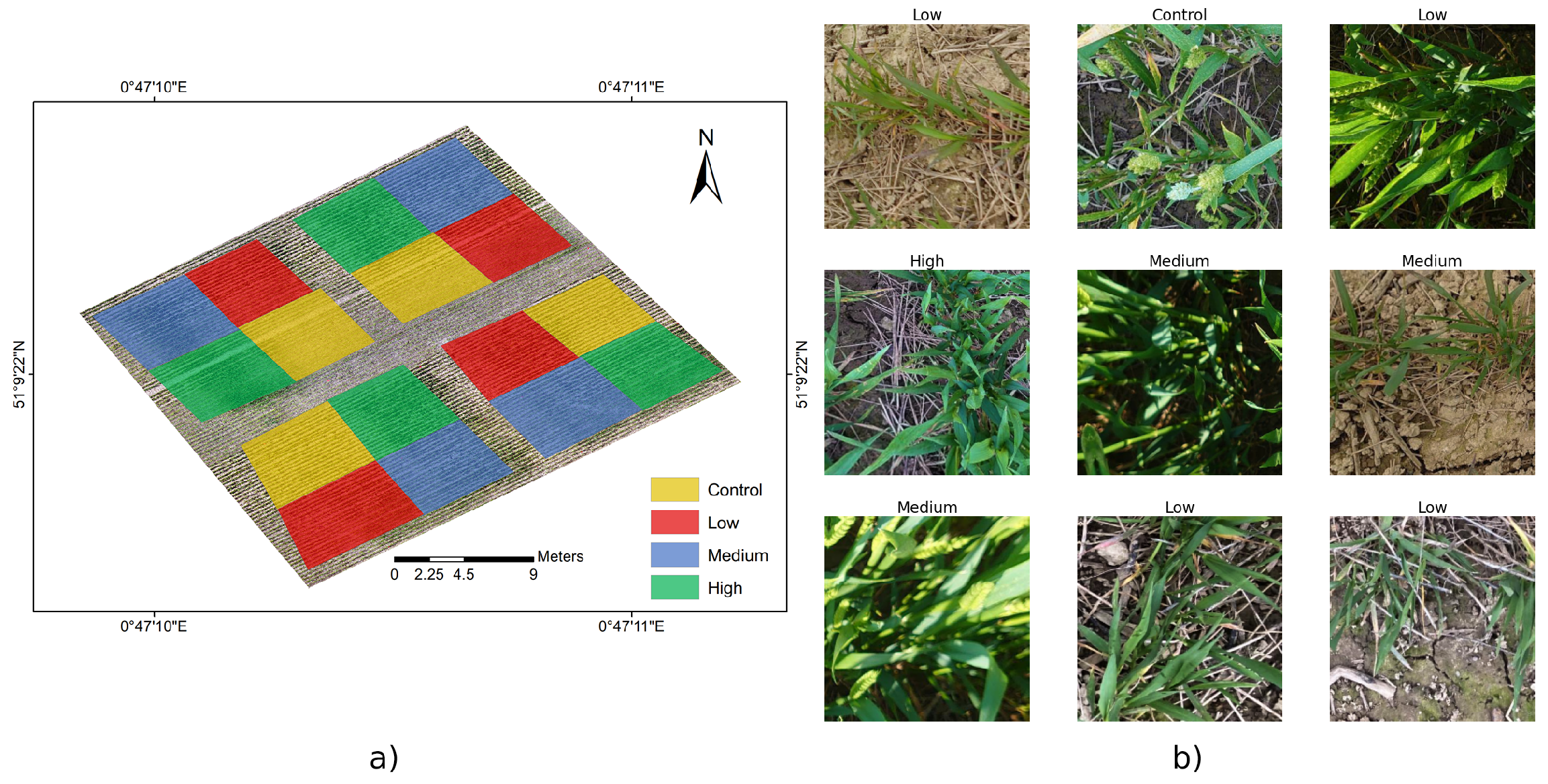
Figure 1. (a) Experimental layout, with plots randomly allocated into four treatments, split into four blocks. Treatments were high (green), medium (blue) and low fertilizer rates (red), and an unfertilized control (yellow). (b) Images collected from different plots with different treatments.
Remotesensing 14 01400 g001
Figure 2. The collected images. The left one is collected near the ground. The right one is collected from the drone.
Remotesensing 14 01400 g002
Figure 3. The structure of the proposed spectral–spatial attention vision transformer (SSVT).
Remotesensing 14 01400 g003
Figure 4. Image augmentations demonstration.
Remotesensing 14 01400 g004
Figure 5. The flowchart of the self-supervised learning.
Remotesensing 14 01400 g005
Figure 6. General network structure and detailed block structure for CNN models.
Remotesensing 14 01400 g006
Figure 7. The Confusion matrix of the classification results achieved by the proposed SSVT (a) without and (b) with self-supervised learning.
Remotesensing 14 01400 g007
Figure 8. The model performance on independent drone datasets captured throughout all growing stages.
Remotesensing 14 01400 g008
Figure 9. The nitrogen status estimation result on drone images captured at the tillering and stem extension stage.
Remotesensing 14 01400 g009
Figure 10. (a) is the original image and (b) is the segmented image without soil. (c) shows the model performance with original and segmented image.
Remotesensing 14 01400 g010
Figure 11. Visualization of the attention map for ResNet and proposed SSVT. The middle column represents the attention map of ResNet. The right column represents the attention map of SSVT.
Remotesensing 14 01400 g011
Figure 12. (a) is the loss converge trend on self-supervised learning, (b) is t-SNE visualization of the model trained with the proposed SSL.
Remotesensing 14 01400 g012
Figure 13. Inference GPU memory usage of ResNet, original ViT, and proposed SSVT.
Remotesensing 14 01400 g013
Table 1. Monitoring schedule and Data collection summary.
Growing StageDateField Image CollectionDrone
Tillering & Stem Extension21-March160
2-April163
9-April177
Heading & Flowering6-May166
14-May177
24-May175
Ripening & Maturity7-June177
22-June177
28-June175
Table 2. OpenDroneMap detailed parameters.
ParameterValue
Camera-lensAuto
CamerasDJI MAVIC pro
Matcher algorithmFast Library for Approximate Nearest Neighbors
Gps-accuracy10 m
Fast-orthophotoTrue
Orthophoto-resolution0.1 and 0.3 cm
Cloud based geotiffTrue
Table 3. The transformer model configuration.
ModelPatch SizeLayerDimensionParam (M)
ViT81238421.67
SSVT81238425.87
Table 4. The proposed model performance comparison with different input sizes under four N treatments.
Image Size 224 × 224
Types of N TreatmentsControlLowMediumHigh
Precision0.9490.9920.9850.923
Recall0.9360.9920.980.941
F1-score0.9430.9920.9820.932
Accuracy0.962
Image Size 384 × 384
Precision0.9730.9910.9820.917
Recall0.9240.9890.9810.964
F1-score0.9480.990.9820.94
Accuracy0.965
Table 5. The performance comparison of the proposed SSVT with the existing conventional models.
Param (M)GFLOPs (GMac)Accuracy (%)
ResNet_5023.524.120.945
EfficientNet_B528.352.40.95
RegNetY-4.0G20.64.10.951
EfficientNetv2_small20.182.870.949
ViT21.674.240.944
SSVT25.874.710.962
Table 6. Model performance without self-supersized learning for the four N treatments.
ModelSSVT w/o SSL
Types of N TreatmentsControlLowMediumHigh
Precision0.9370.8980.7380.784
Recall0.9390.8440.7740.789
F1-score0.9380.870.7560.787
Accuracy0.836
Table 7. Model performance comparison with the proposed model with SBA and the original ViT (four types of N treatment: Control, Low, Medium, and High).
ModelViT
Types of N TreatmentsControlLowMediumHigh
Precisio0.9250.9560.9310.969
Recall0.9940.9750.9440.865
F1-score0.9590.9650.9380.914
Accuracy0.944
ModelSSVT
Precision0.9490.9920.9850.923
Recall0.9360.9920.980.941
F1-score0.9430.9920.9820.932
Accuracy0.962
Table 8. Comparative performance of the classifier vs. five competitors on wheat Nitrogen prediction.
ReferencesModalityObjectiveAccuracy
[72](VI)-based methodsNitrogen use efficiency0.85
[73](VI)-based methodsNitrogen nutrition index0.86
[74]Artificial Neural Network (ANN)/Support Vector Regression (SVR)Leaf nitrogen accumulation0.86
[75]Random ForestChlorophyll content0.89
[37]Random ForestNitrogen nutrition index0.94
Proposed methodSSVTNitrogen status0.96
Publisher’s Note: MDPI stays neutral with regard to jurisdictional claims in published maps and institutional affiliations.