Drivers of Groundwater Change in China and Future Projections

Abstract

Observations worldwide have shown that in recent decades, groundwater depletion intensified notably in many regions. Understanding the interacting drivers of groundwater change enables better human adaptations to climate change and socioeconomic development. Here we use a structural equation model to quantify the contribution of natural and human-induced processes on the groundwater of China by using terrestrial water storage observed by GRACE in combination with climate and socioecological related data at a provincial scale. The results reveal that the influence of climate on groundwater change through indirect impact on the agriculture water consumption is larger than that through direct replenishment. Socioeconomic development contributes in the same order of magnitude as the direct replenishment by climate variabilities to groundwater. In general, forest plays an important role in reserving groundwater at a provincial scale. Based on future climate projections and Shared Socioeconomic Pathways, it is projected that most regions in China will experience a greater groundwater depletion in the future and the variance among regions will become larger.

1. Introduction

Groundwater plays a significant role in sustainable development and is clearly linked to 31% of the attainment of Sustainable Development Goals (SDGs) [1]. The ever-increasing demand of groundwater for agricultural and socioeconomic purposes will serve to stress groundwater depletion in many regions of the world [2,3,4,5]. The impact of climate change, directly through replenishment and indirectly through changes in groundwater use, poses an additional pressure on groundwater resources [6,7,8,9,10,11,12,13]. Investigating the groundwater response to driving factors and make long-term estimations of groundwater storage is therefore crucial for water management.

The relationship between groundwater and its influencing factors has been investigated mainly through statistical methods or hydrological models. Statistical methods including linear regression methods, grey relational analysis, transfer function-noise time series approach, singular spectrum analysis, and wavelet coherence analysis methods have been widely used [11,14,15,16,17,18,19]. Thomas et al. [16] used regression procedures and dominance analysis to explore the relationship between natural and human driving factors and the spatial–temporal changes of groundwater in the United States. The results showed that precipitation showed a higher impact than groundwater extraction. Kuss et al. [17] used singular spectrum analysis, wavelet coherence analysis, and lag correlation analysis to quantify the effects of El Niño Southern Oscillation and North Atlantic Oscillation on precipitation and groundwater in Central Valley, Basin and Range, and North Atlantic Coastal Plain in the United States. The results showed that the groundwater level was partly controlled by inter-annual to multi-decadal climate change, not just a function of temporal patterns in pumping. Liu et al. [20] used one simple attribution analysis to analyze the effect of precipitation and anthropogenic activities on groundwater change. The results showed that precipitation contributed 60% of groundwater storage variability, while human activities, especially socioeconomic development, contributed ~31% of groundwater storage variability. Compared to a statistical approach, hydrological models can reflect the interaction and physical mechanism between climate and hydrology. Brouyère et al. [21] established an integrated hydrological model (MOHISE) to study the direct impact of climate change on the hydrological cycle of the Geer basin in Belgium. The results showed climate change would have a pluri-annual impact on groundwater resources, causing a global “monotonic” decrease in groundwater levels over time. Jyrkama et al. [22] proposed a physical method based on the hydrological model HELP3 to describe the temporal and spatial impact of climate change on groundwater recharge. The results showed that climate change would increase the rate of groundwater recharge and the intensity. Alam et al. [23] combined surface water and groundwater models with climate projection models to evaluate the vulnerability of groundwater in Central Valley California. The results showed that the groundwater would continue to decline in the future since climate change has led to 40–70% more annual groundwater consumption by crops. Wu et al. [24] used a fully coupled climate model to assess the climate-driven impact of potential changes in groundwater storage throughout the 21st century under the RCP8.5 scenario. The results showed that rainfall change in monsoon and humid regions was what most affected groundwater recharging. The regions dominated by snowfall depended on the latitudes and elevation and changes in evapotranspiration were the main determinant of groundwater recharge over dry regions. Li et al. [25] used the Catchment land surface model (CLSM), as well as the WaterGAP and PCR-GLOBWB water resource models combined with GRACE data to simulate the global long-term groundwater storage changes under the influence of non-anthropogenic impacts. The results showed that the variability of the global groundwater was influenced by ENSO’s power over precipitation patterns and global groundwater anomalies were sensitive to precipitation trends.

Those studies above mainly concentrated on the direct impacts of climate change and anthropogenic activities on groundwater, discussing the driving factors of precipitation, temperature, evapotranspiration, groundwater extraction, and other related variables. However, climate change will also affect groundwater changes by indirectly affecting human activities, especially indirectly through land use or land cover changes (mainly through groundwater irrigation) [26]. Research examining the interactions between natural and human-induced process on groundwater change remains limited. Specifically, a comprehensive analysis of the multiple pathways that might influence groundwater disturbances is still lacking in China. Knowledge is limited about the interactions between natural and human-induced processes on groundwater restricted human trade-off adaptations to climate change and socioeconomic growth to mitigate future threats to groundwater provision [27,28].

Here, we use the structural equation model to identify major climate and socioeconomic drivers of the changes of groundwater in China and quantify their contributions. Based on the developed model, we further assess the sensitivity of groundwater storage to future climate and socioeconomic change based on the output from an ensemble of regional circulation models (RCMs) associated with RCP4.5 and RCP8.5 and shared socioeconomic pathways SSP2 and SSP3. The results enable us to design adaptation measures to prevent large groundwater depletion.

2. Materials and Methods

2.1. Analysis of Groundwater Data

We use data from Gravity Recovery and Climate Experiment (GRACE) for the period of 2003–2015 provided by the Jet Propulsion Laboratory mascons (JPL RL05M). The GRACE data are processed using a mass concentration solution that allows for improved spatial resolution and accuracy compared to the spherical harmonic solutions. The spatial resolution of the data is 0.5° × 0.5°. The groundwater anomaly is obtained by subtracting non-groundwater storage (soil moisture, canopy storage, and surface water), which are available from Global Land Data Assimilation System (GLDAS) [29] provided by NASA (GLDAS Noah V2.1). As GRACE data are an anomaly relative to the 2004–2009 time-mean baseline, the soil moisture storage, canopy water storage, and surface water storage from GLDAS are also computed to an anomaly value relative to the same baseline time period. Then we use Equation (1) below to obtain the groundwater storage change based on variable anomaly described above.

$$GWSA=TWSA-SMSA-SWEA-CWSA,$$

(1)

where $GWSA$ suggests the groundwater storage anomaly, $TWSA$ is the terrestrial water storage anomaly, $SMSA$ is the soil-moisture water storage anomaly, $SWEA$ is the snow water equivalent anomaly, and $CWSA$ is the canopy water storage anomaly.

The non-parametric Mann–Kendall trend test [30,31] with Sen’s slope [32] estimator is used to identify the groundwater trend. It calculates the median slopes between all n(n − 1)/2 pairwise combinations of the time series data:

$$T=\mathrm{median}\left(\frac{W_j-W_i}{j-i}\right),$$

(2)

where $T$ is the Theil–Sen median trend, $i$ and $j$ represent different time units (year), and $W_i$ and $W_j$ represent data for different year.

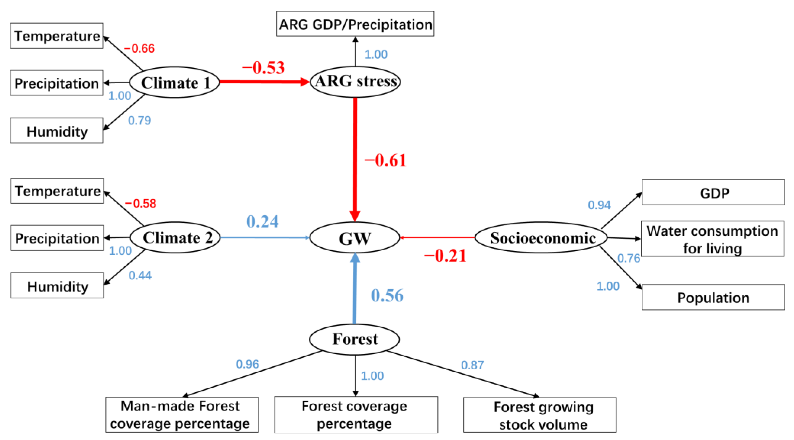
2.2. Structural Equation Model

It is commonly recognized that the direct and indirect forcing of climate variability and change and human activity are main drivers of groundwater change, and the climate influences groundwater through natural and human-induced processes. Here we translate this hypothesized mechanism into a Structural Equation Model (SEM) [33,34] to quantify the magnitude and understand the pathway of how these drivers have contributed to the observed change of groundwater directly or indirectly (Figure 1). SEM has the ability to go beyond the consideration of independent processes (e.g., as in univariate approaches), allowing the examination of simultaneous influences. It has been successfully used to unravel the importance of intercorrelated ecological variables in a variety of applications recently [35,36]. An additional strength of SEM with regard to our study is its ability to incorporate latent variables, i.e., variables that cannot be measured directly but can be expressed by one or more observable indicator variables [37]. Figure 1 shows the conceptual scheme of the proposed SEM model. The model is used to explore two hypotheses [6]: that effects of climate variability and change may be greatest through indirect effects on agricultural water demand, and that groundwater deficit stressed by climate change and socioeconomic growth may be balanced through transforming land-use.

Climate, socioeconomic, agricultural water demand, and land-use factors, the main dimensions of interest in our analysis, are not directly observable (in a strict statistical sense) but can be described by a number of indicator variables. They are therefore incorporated as latent variables in our SEM analysis. The structural model is defined as

$$\eta =B\eta +\Gamma \xi +\mathbf{\zeta },$$

(3)

where $\mathsf{\eta }={\left({\mathsf{\eta }}_1,{\mathsf{\eta }}_2,\dots ,{\mathsf{\eta }}_m\right)}^{\prime }$ denotes the endogenous latent variable (in this paper it refers to the vector of groundwater storages change), $\xi ={\left({\mathsf{\xi }}_1,{\mathsf{\xi }}_2,\dots ,{\mathsf{\xi }}_m\right)}^{\prime }$ is the vector of exogenous latent variables. In this study, we selected climate factor, socioeconomic factor, agricultural stress factor, and forest factor as latent variables and investigate their influence on groundwater. B denotes the matrix of path coefficients that represents the effect of endogenous latent variables on other endogenous latent variables while $\Gamma$ represents the effect of exogenous latent variables on Endogenous Latent Variable and $\mathsf{\zeta }$ represents the inner model residuals. Equation (3) is referred to as being in implicit form because endogenous variables appear on both sides of the equations and have not been “solved”. It is assumed that the diagonal of B is zero so that no element of ${\mathsf{\eta }}_i$ is a function of itself [38]. Equation (3) can be solved for the endogenous variables and written as follows:

$$\left[\begin{array}{c}{\eta }_1\\ {\eta }_2\end{array}\right]=\left[\begin{array}{cc}0& {\beta }_{12}\\ {\beta }_{21}& 0\end{array}\right]\left[\begin{array}{c}{\eta }_1\\ {\eta }_2\end{array}\right]+\left[\begin{array}{cc}{\gamma }_{11}& {\gamma }_{12}\\ {\gamma }_{21}& {\gamma }_{22}\end{array}\right]\left[\begin{array}{c}{\xi }_1\\ {\xi }_2\end{array}\right]+\left[\begin{array}{c}{\zeta }_1\\ {\zeta }_2\end{array}\right],$$

(4)

$$Y={\mathsf{\Lambda }}_y\eta +\epsilon ,$$

(5)

$$X={\mathsf{\Lambda }}_x\xi +\delta .$$

(6)

Each latent variable is represented by observed variables. The observed variable Y for endogenous latent variable can be generated as a linear function of its latent variable $\eta$ and residue $\epsilon$, and $X$ for exogenous latent variables is generated based on $\xi$ and $\delta$. ${\mathsf{\Lambda }}_y$ and ${\mathsf{\Lambda }}_x$ represent the loading matrix, $\epsilon$ and $\delta$ are the measurement errors for Y and X, respectively.

The solution of equations is performed with the Analysis of Moment Structures software (AMOS). All explanatory and response variables were standardized according to their own series before being entered into the model as the following equation:

$${\mathit{v}}_{std}=\frac{\mathit{v}\mathbf{-}\overline{\mathit{v}}}{\mathit{S}{\mathit{D}}_{\mathit{v}}},$$

(7)

where ${\mathit{v}}_{std}$ is the standardized indicator used in the structural equation model, $\mathit{v}$ is the raw variable, $\overline{\mathit{v}}$ is its time series mean, and $\mathit{S}{\mathit{D}}_{\mathit{v}}$ is its standard deviation. This standardization was applied to isolate changes relative to provincial specific mean conditions, and to enable a direct comparison of effects across provinces. It also allowed intercepts to be omitted in the statistical analysis, which grants a more intuitive interpretation of results.

2.3. Description of Observed Variables

The observed variables are collected based on detailed historical inventory data at the provincial scale for the 2003–2015 period. The list and descriptions of potential observed variables are shown in

Table 1. List and description of potential observed variables considered.

Observed Variables	Description	Original Resolution
Temperature	Annual averaged daily records of high temperature	Station
Precipitation	Annual total amount of precipitation	station
Humidity	Annual average daily relative humidity	Station
Forest coverage rate	Annual forest coverage rate	province
Man-made Forest coverage rate	Annual man-made forest coverage rate	province
Forest growing stock	Annual forest growing stock volume per km2	province
Grassland coverage rate	Annual grassland coverage rate	province
Wetland coverage rate	Annual wetland coverage rate	province
Construction land coverage rate	Annual construction land coverage rate	province
Agricultural land coverage rate	Annual agricultural land coverage rate	province
Agricultural GDP	Annual agricultural GDP per km2	province
Yields of main crop products	Annual yields of main crop products per km2	province
Population density	Annual population per km2	province
GDP	Annual Gross Domestic Production per km2	province
Water consumption for living	Annual water consumption for living per km2	province
Water consumption for industry	Annual water consumption for industry per km2	province
Groundwater change	Annual Groundwater change	0.5° × 0.5°

. The climatic indicators used are annual average daily high temperature, annual total amount of precipitation, and annual average daily relative humidity. They are derived from the observation data provided by the National Meteorological Information Center of China. To allow for potential time lags in the effect of climatic drivers on groundwater, the previous year’s temperature and precipitation records are included as explanatory variables. The land-use indicators used include annual forest coverage rate, annual man-made forest coverage rate, annual forest growing stock volume, annual grass coverage rate, annual wetland coverage rate, annual construction land coverage rate, and annual agricultural land coverage rate. Agricultural water demand indicators include annual agricultural GDP per km², sown area of crop, and annual yields of main crop products per km². Socioeconomic indicators include GDP per km², water consumption for living per km², annual water consumption for industry per km², and population per km². These data are available in the China Statistical Yearbook. Additionally, as GRACE data are anomaly relative to the 2004–2009 time-mean baseline, to be consistent, all variables are computed to an anomaly value relative to the 2004–2009 time-mean baseline. The grid variables are unified to the provincial administrative units in China according to the regional mean when constructing the Structural Equation Model.

2.4. Future Scenarios

We use the climate projections provided by the regional climate model NEX-GDDP which are downscaled from Global Climate Models (GCMs) participating in the Coupled Model Intercomparison Project Phase 5 (CMIP5). Climate model outputs of five models are applied: bcc-csm1-1, CanESM2, MIROCESM, IPSL-CM5A-LR, and MPI-ESM-L. The NEX-GDDP only provides outputs of daily gridded highest temperature and precipitation, the humidity is predicted based on the regression of the relationship between humidity and temperature and precipitation. Considering the differences between the model estimates and observed data, we use the bias correction method [39,40,41,42] to adjust climate outputs before predicting future groundwater changes. In this study, the difference between the observed and simulated climate outputs is removed over the baseline period of 2003–2015 according to Equation (8). The advantage of this correction method is that the observed sequence and its linear spatial-, temporal-, and multi-variable dependence structure are naturally preserved [42].

$$T_{MC,year}=T_{Model,year}\times T_{OBS,\mathit{2003}–\mathit{2015}}/T_{Model,\mathit{2003}–\mathit{2015}},$$

(8)

where $T_{MC,year}$ and $T_{Model,year}$ are the corrected and simulated climate outputs for a given year, respectively. $T_{OBS,\mathit{2003}–\mathit{2015}}$ and $T_{Model,\mathit{2003}–\mathit{2015}}$ represent the averaged observed and simulated climate outputs for the period of 2003–2015, respectively.

Future socioeconomic development is taken into consideration by combining the RCPs with shared socioeconomic pathways (SSPs). Two SSPs, the “middle of the road” (i.e., Medium challenges to mitigation and adaptation) (SSP2) and “Regional Rivalry” (i.e., High challenges to mitigation and adaptation) (SSP3), are considered in the study. The SSP2 describes that the globe travels along a path where social, economic, and technological tendencies do not diverge noticeably from past trends. Global population growth is moderate and the second half of the century will see a moderate slowdown in the rate of population growth worldwide. Income disparity is still a problem or is becoming worse slowly. The SSP3 describes that countries are being pushed to concentrate more on internal or, at most, regional issues by a resurgence of nationalism, worries about competitiveness and security, and regional conflicts. Population growth is high in emerging nations and low in industrialized nations [43].

3. Results

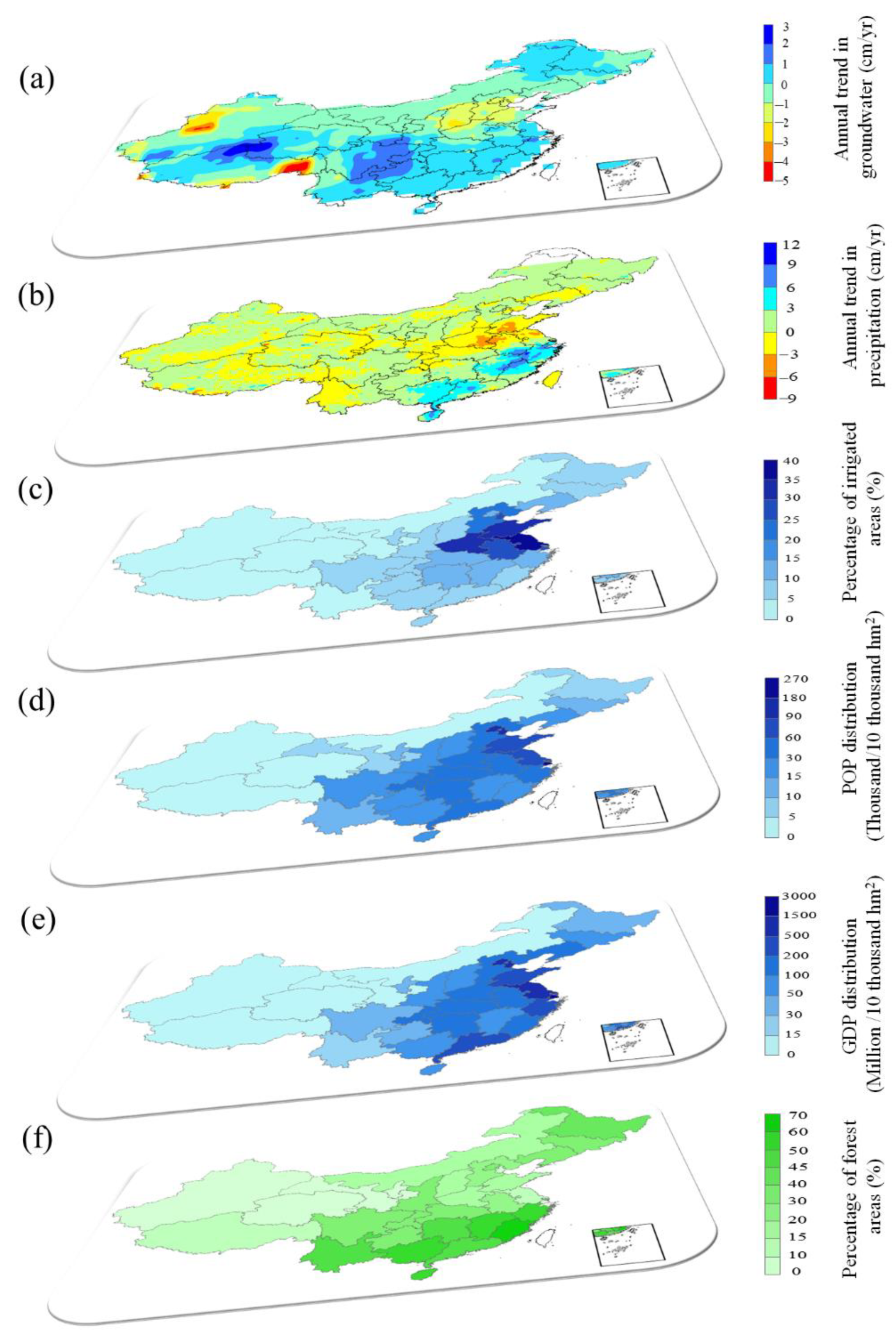
3.1. Changes in Groundwater and Main Influencing Variables

We quantify trends in groundwater storage in China observed by Gravity Recovery and Climate Experiment (GRACE) [6,44] satellites during 2003–2015 (Figure 1). The groundwater storage has declined in northern China at an average rate of −0.204 cm yr⁻¹ and increased by 0.431 cm yr⁻¹ in southern China between 2003 and 2015. Significant declines in groundwater anomalies are observed in Tien Shan regions in northwestern China’s Xinjiang Province, South of Tibet, and North China Plain. The largest depletion rate reached −4.61 cm yr⁻¹ during the study period.

Groundwater storage depletion occurs when the water extraction rate is larger than that of recharge [4]. Precipitation is the primary recharger of groundwater and is strongly affected by climate variability [6]. During 2003–2015, the observed change in groundwater storage increases in southern China is partially attributable to the abundant precipitation, which increases 12.46 mm yr⁻¹ in average throughout the study period (Figure 1). While the precipitation of northern China showed a slightly increasing trend or a declining trend, especially in the southern part of the North China Plain (−14.32 mm yr⁻¹). The North China Plain is the first most heavily irrigated region and is among China’s most populated and economically strongest regions (see Figure 2). Furthermore, we can see southern China has a larger forest coverage rate compared to its northern part. An intuitive understanding is that the socioeconomic and agricultural related drivers and changes in precipitation contribute together to the negative trend in groundwater storage. Their contributions and coupling effect on groundwater, however, remain unclear. An understanding of the relationship between different drivers and groundwater change is consequential to the development of robust estimates of not only groundwater recharge and depletion but of a strategic plan for balancing groundwater storage under climate changes and socioeconomic development.

3.2. Relative Contribution of Driving Factors

Figure 3 shows the estimation of the SEM model with a total of 13 manifest observed variables. Other observed variables, especially variables related to land-use, such as wetland coverage rate, construction land coverage rate, and grassland coverage rate, are not significant and resulted in a fairly poor model–data fit. As shown in Figure 3, Climate 1 indicates climate variabilities in the current year and Climate 2 indicates climate variabilities in the previous year. Socioeconomic indicates socioeconomic development. Agricultural stress (ARG stress) is defined as the ratio between Agricultural GDP per km² and precipitation per km². We use forest as the latent variable instead of land-use as the manifest observed variables of land-use are highly related to forest. Red and blue arrows represent negative and positive paths from latent variables to groundwater (GW), respectively. Boxes represent observed variables and the path coefficient of black arrows indicates the importance of observed variable to represent the corresponding latent variable. The observed variable with a path value of 1 is selected as a reference, and the value of other paths indicate their contribution to the latent variable relative to the referenced observed variable. The larger the absolute value is, the stronger the influence is.

The entire model has an adequate goodness of fit based on Normed chi-square (NC): 4.99 and Goodness-of-fit index (GFI): 0.90. The mechanistic understanding of groundwater change is as following: Climate influences the groundwater directly through recharging: a combination of heavy rainfall, high humidity, and low temperature frequently results in increasing trend of groundwater change. Climate indirectly influences groundwater change through irrigation demand. The larger the ARG stress, the greater the groundwater demand for agricultural irrigation. Less precipitation leads to more extensive irrigation activities and therefore increases groundwater depletion stress. Socioeconomic development, including expanding economy and population, increases groundwater demand. The influence of forest on groundwater is controversial and it is difficult to quantify impacts of vegetation change on groundwater yield [45]. One perception is that trees benefit water availability [28,46]. However, it is also doubted that planting could worsen water scarcity by using a lot of water [44].

Our results show that the direct impact of the climate factor on groundwater is mainly through the recharge from the previous year (standard coefficient 0.24). Climate variabilities of the current year notably influence groundwater through indirect effects on agricultural irrigation stress (standard coefficient −0.61). Socioeconomic development contributed negatively to the change of groundwater (standard coefficient −0.21). Forest has a positive influence on groundwater with a magnitude comparative to that of the agricultural irrigation stress (standard coefficient 0.56). Analyzing latent variables individually, we find that higher precipitation and humidity lead to a higher level of groundwater storage than expected. Furthermore, higher temperature increases the rate of evaporation and decreases groundwater storage. Economic development and population expansion are equally influential and exerted a significant negative influence on groundwater storage. All variables related to forest are found to enhance groundwater recharge.

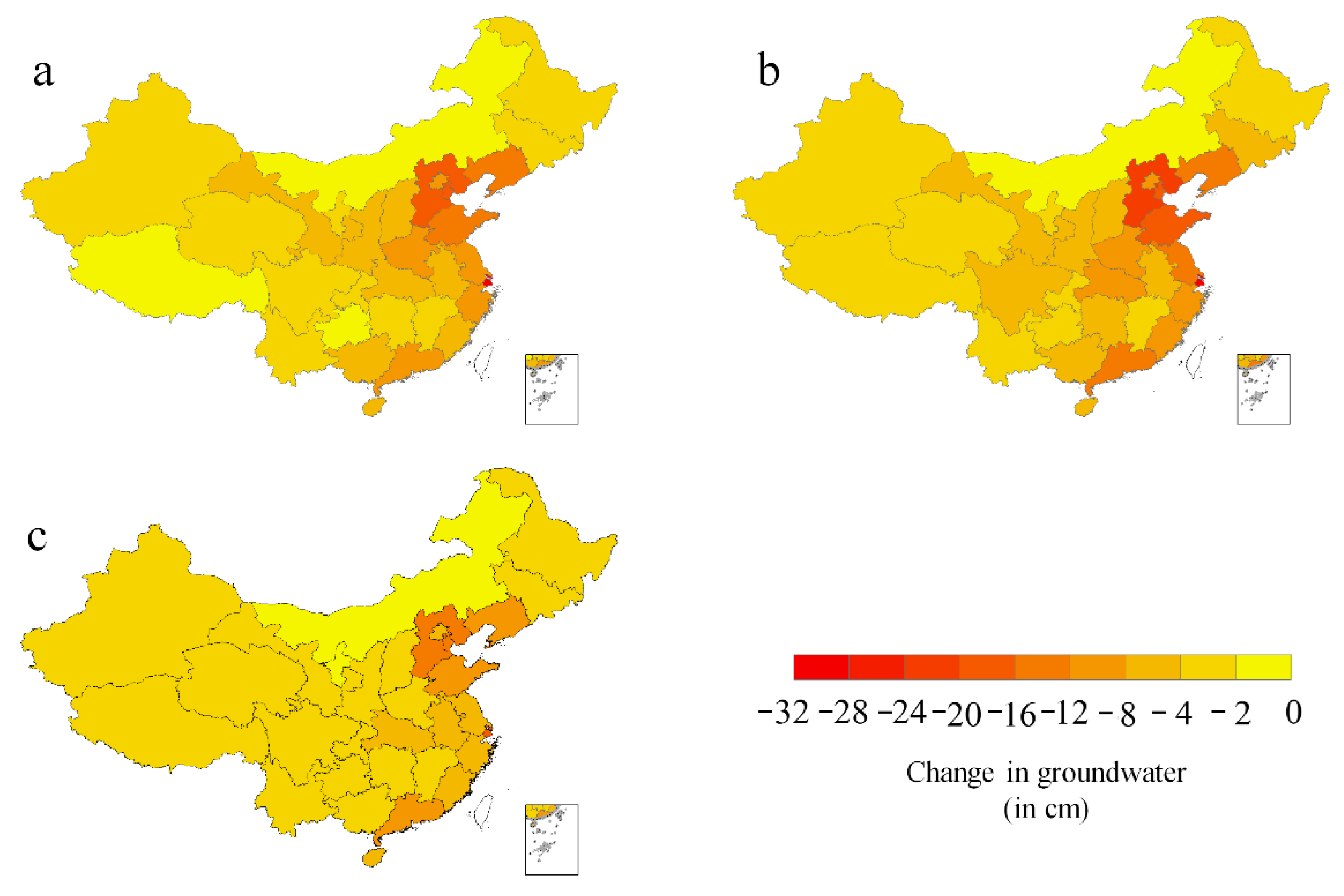
3.3. Groundwater Sensitivity to a Changing Future

The parameterized SEM model allows us to analyze sensitivity of groundwater storage to potential future climate and socioeconomic change. Here, we define mean state of climate and socioeconomic records for the period of 2003–2015 as the baseline, to quantify the sensitivity of groundwater storage facing a changing future. Three time periods—Near-term (2030, pooling 2020–2039 data), Mid-term (2050, pooling 2040–2059 data), and Long-term (2090, polling 2081–2099)—and three combined climate and socioeconomic scenarios—optimistic (RCP4.5 and SSP2), business-as-usual (RCP8.5 and SSP2), and pessimistic from IPCC (RCP8.5 and SSP3)—are considered. The bias-corrected Climate outputs from five downscaled climate projections (NEX-GDDP) [47] generated from GCMs which well reproduce the observed climate historical records over China are applied (see Materials and Methods). NEX-GDDP projects clearly the increase of mean temperature over the whole of China in the future, e.g., by Mid-term, the overall average highest temperature is projected to become warmer by 1.7 °C and 2.6 °C across China relative to the 2003–2015 baseline by average of model ensemble for RCP 4.5 and RCP 8.5, respectively. Moreover, northern China is warming faster than southern China. Such a rising temperature would inevitably enhance evaporation and would serve to stress limited groundwater resources further, through direct depletion and indirect agricultural water stress. According to regional climate models, the precipitation shows an increasing trend of precipitation for most parts of China. The RCP4.5 ensembles mean projects an average of 30 mm (8%) and 83 mm (7%) increases in average annual precipitation in northern China and southern China in Mid-term compared with 2003–2015, respectively.

An expanding population, coupled with economic development, is bound to change future demand for groundwater in China. The SSPs [48] project continued a U-shape population and economic growth: e.g., in the “middle-of-the-road” SSP2, population of China will increase by 3.85%, −7.29%, and −40.52% in 2030, 2050, and 2090 relative to 2003–2015 mean; while GDP is 3.7, 5.6, and 6.3 times larger over the same period, resulting in a greater demand on the groundwater.

On the basis of RCPs and SSPs, we use the SEM model to analyze the change of groundwater storage if the current mean state of the 2003–2015 period is changed to that of three combined climate and socioeconomic scenarios in 2030, 2050, and 2090, respectively (Figure 4). The magnitude and spatial pattern of groundwater changes vary with the scenarios; however, all scenarios suggest a decrease in groundwater. Although precipitation increases in most regions in China, its effect is dwarfed by the impact of the more rapid growth of economic activities in urban areas. Groundwater decreases the largest in the business-as-usual scenario, because of its relatively higher projected temperature, lower projected precipitation, and higher socioeconomic development, leading to a higher impact of groundwater change. The model ensemble suggests an average change of −1.7 cm, −3.9 cm, −4.7 cm by 2030, 2050, and 2090 under optimistic scenario, respectively, decreases −2.1 cm, −4.7 cm, −7.7 cm for business-as-usual scenario, and −1.8 cm, −3.4 cm, −5.9 cm for pessimistic scenario. Meanwhile, it is found that large geographical differences exist across the country. Under future scenarios, the decrease of groundwater would concentrate much more in coastal economic zones, which are mostly due to socioeconomic change and can be explained by the disproportionate economic growth between regions in SSP scenarios. For example, Shanghai is expected to experience the largest groundwater decrease in comparison to other regions, largely attributed to its projected higher socioeconomic growth rate. The annual GDP of Shanghai increases from over US$0.23 trillion currently, to up to US$1.16 trillion in 2050 in the SSP2 ‘Middle of the Road’ projection. The North China Plain is also expected to face a large increase in economic growth (409% rise by 2050 in the SSP2 ‘Middle of the Road’ projection compared to that of 2003–2015). The total increased water requirement imposed by socioeconomic development will exceed increases in projected rainfall, leading to a continuing trend towards severe deficit on groundwater in the North China Plain. As the North China Plain is one of the most prosperous regions and serves as one of the largest cropland in China, a high conflict between the urban and agricultural sectors is expected and reconcilement is needed to balance their development.

4. Discussion

Our study is a pioneer research in investigating the interactions between natural and human-induced processes on groundwater change using the SEM approach. By using SEM, we are able to quantify the direct and indirect contributions of different drivers on groundwater storage. The pathways among climate variability, anthropogenic factors, and groundwater storage variations were previously unrecognized. Interestingly, it is for the first time we found that in general forest has a positive influence on groundwater at the provincial scale of China, although it was pointed out that revegetation in some semi-arid Loess Plateau in China has increased evapotranspiration and hence decreases groundwater [49]. As we show in the results, generally, groundwater is benefited from more forest coverage for most regions of China, likely owing to the fact that forests improve soil hydraulic conductivity and impede evaporation which outweigh their extra water use [45].

However, due to the complex and dynamic nature of the groundwater change, detailed analysis in local level is needed for a refined design of vegetation species and density by considering local conditions. We acknowledge that there are some uncertainties in simulated components (SMSA, SWEA, CWSA) from GLDAS and limitations due to a lack of surface water storage anomaly. Moreover, due to the short time period from 2003–2015, it may not completely reveal various mechanisms that influence groundwater storage change. Nevertheless, our findings provide useful information about potential future groundwater situations and have important policy implications for making decisions at the national and provincial scales for reaching a sustainable development.

Furthermore, we acknowledge that in this study we only considered main driving factors that influence groundwater storage, and the estimated future groundwater change only reflects its response to the selected factors. For example, in our model we were unable to consider the effect of south-to-north water diversion in China. Yang et al. [50] used a high-resolution community water model combining water diversion, water use, and climate variability indicators to predict groundwater storage changes in the North China Plain during the 2019–2050 time period. The result showed that groundwater in the North China Plain would decline further without considering the impact of future south-to-north water diversion. Moreover, water diversion combined with decreasing water use can result in stabilized groundwater storage in the future. How to incorporate water management measures in our model will be explored in our future study.

5. Conclusions

In this study, we use a structural equation model to capture how groundwater is influenced by driving factors and respond to future climate change. Our work shows that the direct impact of climate factor on groundwater is mainly through the recharge from the previous year. Climate variabilities of the current year notably influences groundwater through indirect effects on agricultural irrigation stress. Socioeconomic development and agricultural irrigation contributed negatively to the change of groundwater. Forest has a positive influence on groundwater with a magnitude comparative to that of the agricultural irrigation stress.

The results of sensitivity of groundwater storage to future climate and socioeconomic change show that both global warming and socioeconomic growth are inevitably increasing pressure of regional groundwater recession. The groundwater of China will face a decrease. Under future scenarios, the groundwater in coastal economic zones is more vulnerable due to increasing water requirement imposed by socioeconomic development. Sustainable groundwater management policies should be implemented to cope with future stresses.

References

1. Guppy, L.; Uyttendaele, P.; Villholth, K.G.; Smakhtin, V. Groundwater and Sustainable Development Goals: Analysis of Interlinkages; UNU-INWEH Report Series, Issue 04; United Nations University: Tokyo, Japan, 2018. [Google Scholar]
2. Rodell, M.; Famiglietti, J.S.; Wiese, D.N.; Reager, J.; Beaudoing, H.K.; Landerer, F.W.; Lo, M.-H. Emerging trends in global freshwater availability. Nature 2018, 557, 651–659. [Google Scholar] [PubMed]
3. Rodell, M.; Velicogna, I.; Famiglietti, J.S. Satellite-based estimates of groundwater depletion in India. Nature 2009, 460, 999–1002. [Google Scholar] [CrossRef] [PubMed]
4. Aeschbach-Hertig, W.; Gleeson, T. Regional strategies for the accelerating global problem of groundwater depletion. Nat. Geosci. 2012, 5, 853–861. [Google Scholar] [CrossRef]
5. Wada, Y.; Wisser, D.; Bierkens, M.F. Global modeling of withdrawal, allocation and consumptive use of surface water and groundwater resources. Earth Syst. Dyn. 2014, 5, 15–40. [Google Scholar] [CrossRef]
6. Taylor, R.G.; Scanlon, B.; Döll, P.; Rodell, M.; Van Beek, R.; Wada, Y.; Longuevergne, L.; Leblanc, M.; Famiglietti, J.S.; Edmunds, M. Ground water and climate change. Nat. Clim. Chang. 2013, 3, 322–329. [Google Scholar] [CrossRef]
7. Gurdak, J.J. Climate-induced pumping. Nat. Geosci. 2017, 10, 71. [Google Scholar] [CrossRef]
8. Meixner, T.; Manning, A.H.; Stonestrom, D.A.; Allen, D.M.; Ajami, H.; Blasch, K.W.; Brookfield, A.E.; Castro, C.L.; Clark, J.F.; Gochis, D.J. Implications of projected climate change for groundwater recharge in the western United States. J. Hydrol. 2016, 534, 124–138. [Google Scholar] [CrossRef]
9. Thomas, B.F.; Behrangi, A.; Famiglietti, J.S. Precipitation intensity effects on groundwater recharge in the southwestern United States. Water 2016, 8, 90. [Google Scholar] [CrossRef]
10. Russo, T.A.; Lall, U. Depletion and response of deep groundwater to climate-induced pumping variability. Nat. Geosci. 2017, 10, 105–108. [Google Scholar] [CrossRef]
11. Asoka, A.; Gleeson, T.; Wada, Y.; Mishra, V. Relative contribution of monsoon precipitation and pumping to changes in groundwater storage in India. Nat. Geosci. 2017, 10, 109–117. [Google Scholar]
12. Green, T.R.; Taniguchi, M.; Kooi, H.; Gurdak, J.J.; Allen, D.M.; Hiscock, K.M.; Treidel, H.; Aureli, A. Beneath the surface of global change: Impacts of climate change on groundwater. J. Hydrol. 2011, 405, 532–560. [Google Scholar] [CrossRef] [Green Version]
13. Earman, S.; Dettinger, M. Potential impacts of climate change on groundwater resources–a global review. J. Water Clim. Chang. 2011, 2, 213–229. [Google Scholar] [CrossRef]
14. Wang, T.-Y.; Wang, P.; Zhang, Y.-C.; Yu, J.-J.; Du, C.-Y.; Fang, Y.-H. Contrasting groundwater depletion patterns induced by anthropogenic and climate-driven factors on Alxa Plateau, northwestern China. J. Hydrol. 2019, 576, 262–272. [Google Scholar] [CrossRef]
15. Ojeda Olivares, E.A.; Sandoval Torres, S.; Belmonte Jiménez, S.I.; Campos Enríquez, J.O.; Zignol, F.; Reygadas, Y.; Tiefenbacher, J.P. Climate change, land use/land cover change, and population growth as drivers of groundwater depletion in the central valleys, Oaxaca, Mexico. Remote Sens. 2019, 11, 1290. [Google Scholar] [CrossRef]
16. Thomas, B.F.; Famiglietti, J.S. Identifying climate-induced groundwater depletion in GRACE observations. Sci. Rep. 2019, 9, 4124. [Google Scholar] [CrossRef]
17. Kuss, A.J.M.; Gurdak, J.J. Groundwater level response in US principal aquifers to ENSO, NAO, PDO, and AMO. J. Hydrol. 2014, 519, 1939–1952. [Google Scholar] [CrossRef]
18. Li, X.; Li, G.; Zhang, Y. Identifying major factors affecting groundwater change in the North China Plain with grey relational analysis. Water 2014, 6, 1581–1600. [Google Scholar] [CrossRef]
19. Van Dijk, W.M.; Densmore, A.L.; Jackson, C.R.; Mackay, J.D.; Joshi, S.K.; Sinha, R.; Shekhar, S.; Gupta, S. Spatial variation of groundwater response to multiple drivers in a depleting alluvial aquifer system, northwestern India. Prog. Phys. Geogr. Earth Environ. 2020, 44, 94–119. [Google Scholar] [CrossRef]
20. Liu, K.; Li, X.; Long, X. Trends in groundwater changes driven by precipitation and anthropogenic activities on the southeast side of the Hu Line. Environ. Res. Lett. 2021, 16, 094032. [Google Scholar] [CrossRef]
21. Brouyère, S.; Carabin, G.; Dassargues, A. Climate change impacts on groundwater resources: Modelled deficits in a chalky aquifer, Geer basin, Belgium. Hydrogeol. J. 2004, 12, 123–134. [Google Scholar] [CrossRef]
22. Jyrkama, M.I.; Sykes, J.F. The impact of climate change on spatially varying groundwater recharge in the grand river watershed (Ontario). J. Hydrol. 2007, 338, 237–250. [Google Scholar] [CrossRef]
23. Alam, S.; Gebremichael, M.; Li, R.; Dozier, J.; Lettenmaier, D.P. Climate change impacts on groundwater storage in the Central Valley, California. Clim. Chang. 2019, 157, 387–406. [Google Scholar] [CrossRef]
24. Wu, W.-Y.; Lo, M.-H.; Wada, Y.; Famiglietti, J.S.; Reager, J.T.; Yeh, P.J.-F.; Ducharne, A.; Yang, Z.-L. Divergent effects of climate change on future groundwater availability in key mid-latitude aquifers. Nat. Commun. 2020, 11, 3710. [Google Scholar] [CrossRef] [PubMed]
25. Li, B.; Rodell, M.; Sheffield, J.; Wood, E.; Sutanudjaja, E. Long-term, non-anthropogenic groundwater storage changes simulated by three global-scale hydrological models. Sci. Rep. 2019, 9, 14179. [Google Scholar] [CrossRef]
26. Amanambu, A.C.; Obarein, O.A.; Mossa, J.; Li, L.; Ayeni, S.S.; Balogun, O.; Oyebamiji, A.; Ochege, F.U. Groundwater system and climate change: Present status and future considerations. J. Hydrol. 2020, 589, 125163. [Google Scholar] [CrossRef]
27. Cuthbert, M.; Gleeson, T.; Moosdorf, N.; Befus, K.M.; Schneider, A.; Hartmann, J.; Lehner, B. Global patterns and dynamics of climate–groundwater interactions. Nat. Clim. Chang. 2019, 9, 137–141. [Google Scholar] [CrossRef]
28. Flörke, M.; Schneider, C.; McDonald, R.I. Water competition between cities and agriculture driven by climate change and urban growth. Nat. Sustain. 2018, 1, 51–58. [Google Scholar] [CrossRef]
29. Rodell, M.; Houser, P.; Jambor, U.; Gottschalck, J.; Mitchell, K.; Meng, C.; Arsenault, K.; Cosgrove, B.; Radakovich, J.; Bosilovich, M. The global land data assimilation system. Bull. Am. Meteorol. Soc. 2004, 85, 381–394. [Google Scholar] [CrossRef]
30. Mann, H.B. Nonparametric tests against trend. Econom. J. Econom. Soc. 1945, 13, 245–259. [Google Scholar] [CrossRef]
31. Kendall, M.G. Rank Correlation Methods; Griffin: Oxford, England, 1948; Available online: https://psycnet.apa.org/record/1948-15040-000 (accessed on 10 June 2018).
32. Theil, H. A rank-invariant method of linear and polynomial regression analysis. Indag. Math. 1950, 12, 173. [Google Scholar]
33. Maruyama, G. Basics of Structural Equation Modeling; Sage: Thousand Oaks, CA, USA, 1998. [Google Scholar]
34. Grace, J.B. Structural Equation Modeling and Natural Systems; Cambridge University Press: Cambridge, UK, 2006. [Google Scholar]
35. Jonsson, M.; Wardle, D.A. Structural equation modelling reveals plant-community drivers of carbon storage in boreal forest ecosystems. Biol. Lett. 2010, 6, 116–119. [Google Scholar] [CrossRef] [PubMed]
36. Youngblood, A.; Grace, J.B.; McIver, J.D. Delayed conifer mortality after fuel reduction treatments: Interactive effects of fuel, fire intensity, and bark beetles. Ecol. Appl. 2009, 19, 321–337. [Google Scholar] [CrossRef] [PubMed] [Green Version]
37. Grace, J.B.; Anderson, T.M.; Olff, H.; Scheiner, S.M. On the specification of structural equation models for ecological systems. Ecol. Monogr. 2010, 80, 67–87. [Google Scholar] [CrossRef]
38. Wall, M.M.; Amemiya, Y. Nonlinear structural equation modeling as a statistical method. In Handbook of Latent Variable and Related Models; Elsevier: Amsterdam, The Netherlands, 2007; pp. 321–343. [Google Scholar]
39. Rosenzweig, C. Potential CO2-induced climate effects on North American wheat-producing regions. Clim. Chang. 1985, 7, 367–389. [Google Scholar] [CrossRef]
40. Santer, B. The use of general circulation models in climate impact analysis—a preliminary study of the impacts of a CO2-induced climatic change on West European agriculture. Clim. Chang. 1985, 7, 71–93. [Google Scholar] [CrossRef]
41. Gleick, P.H. Methods for evaluating the regional hydrologic impacts of global climatic changes. J. Hydrol. 1986, 88, 97–116. [Google Scholar] [CrossRef]
42. Maraun, D. Bias correcting climate change simulations-a critical review. Curr. Clim. Chang. Rep. 2016, 2, 211–220. [Google Scholar] [CrossRef]
43. Riahi, K.; Van Vuuren, D.P.; Kriegler, E.; Edmonds, J.; O’neill, B.C.; Fujimori, S.; Bauer, N.; Calvin, K.; Dellink, R.; Fricko, O. The shared socioeconomic pathways and their energy, land use, and greenhouse gas emissions implications: An overview. Glob. Environ. Chang. 2017, 42, 153–168. [Google Scholar] [CrossRef]
44. Rodell, M.; Famiglietti, J. Detectability of variations in continental water storage from satellite observations of the time dependent gravity field. Water Resour. Res. 1999, 35, 2705–2723. [Google Scholar] [CrossRef]
45. Ilstedt, U.; Tobella, A.B.; Bazié, H.; Bayala, J.; Verbeeten, E.; Nyberg, G.; Sanou, J.; Benegas, L.; Murdiyarso, D.; Laudon, H. Intermediate tree cover can maximize groundwater recharge in the seasonally dry tropics. Sci. Rep. 2016, 6, 21930. [Google Scholar] [CrossRef]
46. Tapley, B.D.; Bettadpur, S.; Watkins, M.; Reigber, C. The gravity recovery and climate experiment: Mission overview and early results. Geophys. Res. Lett. 2004, 31, 4. [Google Scholar] [CrossRef]
47. Bao, Y.; Wen, X. Projection of China’s near-and long-term climate in a new high-resolution daily downscaled dataset NEX-GDDP. J. Meteorol. Res. 2017, 31, 236–249. [Google Scholar] [CrossRef]
48. Warszawski, L.; Frieler, K.; Huber, V.; Piontek, F.; Serdeczny, O.; Schewe, J. The inter-sectoral impact model intercomparison project (ISI–MIP): Project framework. Proc. Natl. Acad. Sci. USA 2014, 111, 3228–3232. [Google Scholar] [CrossRef] [PubMed]
49. Feng, X.; Fu, B.; Piao, S.; Wang, S.; Ciais, P.; Zeng, Z.; Lü, Y.; Zeng, Y.; Li, Y.; Jiang, X. Revegetation in China’s Loess Plateau is approaching sustainable water resource limits. Nat. Clim. Chang. 2016, 6, 1019–1022. [Google Scholar] [CrossRef]
50. Yang, W.; Long, D.; Scanlon, B.R.; Burek, P.; Zhang, C.; Han, Z.; Butler Jr, J.J.; Pan, Y.; Lei, X.; Wada, Y. Human intervention will stabilize groundwater storage across the North China Plain. Water Resour. Res. 2022, 58, e2021WR030884. [Google Scholar] [CrossRef]
Figure 1. Conceptual scheme of the proposed SEM model for exploring the direct and indirect effects on groundwater (GW) of climate variability, socioeconomic development, agricultural water demand (AGD), and land-use.
Remotesensing 14 04825 g001
Figure 2. Trend in groundwater and main supporting data maps during 2003–2015. (Top to Bottom) (a) Annual trend in groundwater anomaly based on GRACE (in centimeters per year); (b) changes in precipitation (in centimeters per year); (c) percentage of irrigated areas (in percent); (d) GDP (in Million $ per 10 thousand hectares); (e) population (in thousand per 10 thousand hectares); (f) percentage of forest areas (in percent).
Remotesensing 14 04825 g002
Figure 3. Structural equation model for groundwater-drivers relations.
Remotesensing 14 04825 g003
Figure 4. Mean changes in groundwater storage projected for (a) optimistic scenarios RCP4.5 and SSP2 (b) business-as-usual scenarios RCP8.5 and SSP2 and (c) pessimistic scenarios RCP8.5 and SSP3. Changes are represented by difference in groundwater between future (2041–2050) and current (2003–2015).
Remotesensing 14 04825 g004