Characterizing and Modeling Tropical Sandy Soils through VisNIR-SWIR, MIR Spectroscopy, and X-ray Fluorescence

Abstract

Despite occupying a large area of the globe and being the next agricultural frontier, sandy soils are seldom explored in scientific studies. Considering the high capacity of remote sensing in soil characterization, this work aimed to: (i) characterize sandy soils’ profiles from proximal sensing; (ii) assess the ability of visible, near, and short-wave infrared (Vis-NIR-SWIR) as well as mid-infrared (MIR) spectroscopy to distinguish soil classes of highly sandy content; (iii) quantify physical and chemical attributes of sandy soil profiles from Vis-NIR-SWIR and MIR spectroscopy as well as X-ray fluorescence (pXRF). Samples were described and collected from 29 sandy soil profiles. The 127 samples went under Vis-NIR-SWIR and MIR spectroscopy, X-ray fluorescence, and chemical and physical analyses. The spectra were analyzed based on “Morphological Interpretation of Reflectance Spectrum” (MIRS), Principal Components Analysis (PCA), and cluster methodology to characterize soils. The integration of different information obtained by remote sensors, such as Vis-NIR-SWIR, MIR, and Portable X-ray Fluorescence (pXRF), allows for pedologically complex characterizations and conclusions in a short period and with low investment in analysis and reagents. The application of MIRS concepts in the VNS spectra of sandy soils showed high potential for distinguishing pedological classes of sandy soils. The MIR spectra did not show distinct patterns in the general shapes of the curves and reflectance intensities between sandy soil classes. However, even so, this region showed potential for identifying mineralogical constitution, texture, and OM contents, assuming high importance for the complementation of soil pedometric characterizations using VNS spectroscopy. The VNS and MIR data, combined or isolated, showed excellent predictive performance for the estimation of sandy soil attributes (R² > 0.8). Sandy soil color indices, which are very important for soil classification, can be predicted with excellent accuracy (R² from 0.74 to 0.99) using VNS spectroscopy or the combination of VNS + MIR.

1. Introduction

The soil is formed by a combination of environmental factors, source material, climate, relief, organisms, and time, in a process called pedogenesis. According to the functional-factorial model described by Dokuchaev and equated by [1], the interaction between the source material and climate in a certain position of the landscape conditions the emergence and development of organisms, which, over time, induces the processes of evolution and formation/transformation of soils. The process of soil evolution generates chemical and physical changes in the soil matrix that change, for example, the proportions of its textural fractions of sand, silt, and clay.

Sandy soils, mainly formed by the sand fraction, generally refer to poorly developed soils, according to the Brazilian Soil Classification System (SiBCS) [2]. This low degree of development, or low weathering rate, of the sandy soils may be related to the source material resistance to weathering, relief, climate, and the low capacity of action of the organisms in the system. Thus, despite having in common a large amount of sand, sandy soils are very different among themselves.

The wide range of different sandy soils provides several uses possibilities for these soils [3]. However, the difficult characterization and/or lack of targeted studies cause, in practice, sandy soils to be considered as a single and simple group, with no degrees of aptitude/usage capabilities. According to [2], sandy soils can form different pedological classes depending on the depth of the profile, depth of the sandy layers, the textural gradient between horizons, degree of structuring, color, hydromorphic conditions, etc. [2]. Beyond the different pedological classes, according to [3], sandy soils can be distinct and, hence, have different usage capabilities depending on dynamics, organic matter content, clay content, clay fraction mineralogy, proportions of the sand fractions, and water retention capacity. Considering that sandy soils occupy 7% of the world’s surface [4], 8% of the Brazilian territory, and 15% of the Cerrado (a biome that covers 13 Brazilian states, in an area of about 200 million hectares, being the richest savanna in the world in terms of diversity and the second largest biome in the country), the crop expansion has been concentrated in sandy soils as in the MATOPIBA region (frontier region of Maranhão, Tocantins, Piauí, and Bahia states), which is the main Brazilian agricultural frontier [3].

Since sandy soils are being considered as crop environments, developing and implementing methodologies that allow for more accurate and quicker characterizations are paramount. Therefore, proximal sensing has proven to be an excellent tool due to its high sensitivity to mineral and organic constituents and its capacity to predict physical, chemical, and physical-hydric attributes. Proximal sensing (carried out in the laboratory, under controlled conditions) is also reagent independent, low cost, and has a fast execution.

According to [5,6,7,8,9,10,11,12], there is a high capacity of visible, near-infrared, and short-wave infrared (VNS), as well as medium-infrared (MIR) spectroscopy to identify soil classes. Ref [13] developed a series of criteria for morphological analysis and classification of VNS spectra relating them to their textural classes, mineral constituents, and pedological classes. Few studies have used the MIR region for descriptive analysis. Refs [9,14,15,16,17,18,19,20,21,22,23] proved that VNS and MIR spectroscopy and X-ray fluorescence have an excellent accuracy for estimating chemical and physical soil attributes. Ref [10] demonstrated that even machine learning techniques (such as Cluster and Principal Component Analysis—PCA) are efficient to automatically categorize/classify soils based only on remote sensing information.

Despite the numerous and vast studies for the characterization of pedological classes based on proximal sensing, estimation of attributes, and even the development of spectral libraries at national levels [5,8,15,24] and worldwide [25], no study has specifically focused on sandy soils characterization. Thus, aiming to initiate efforts to characterize tropical sandy soils through proximal sensing, this study aimed: (I) to characterize sandy soil profiles using proximal sensing; (II) to evaluate the ability of VNS and MIR spectroscopy to distinguish soil classes with high sand content using the “Morphological interpretation of reflectance spectrum” (MIRS) methodology; and (III) quantify physical and chemical attributes of sandy soil profiles using VNS and MIR spectroscopy and X-ray fluorescence (pXRF).

2. Materials and Methods

A summary of the methodological flow is presented in Section 2 and, sequentially, in Section 2.1,Section 2.2,Section 2.3,Section 2.4 and Section 2.5, the methodology details are presented. This study was carried out based on 29 soil profiles distributed in the Mato Grosso state (Figure 1). These profiles were classified, and all horizons were sampled. The samples were submitted to physical, chemical, and spectral analysis (Vis-NIR-SWIR-MIR and pXRF). Subsequently, the data obtained were used for characterization of soil classes (using MIRS, PCA, and Cluster methodologies) and for chemical and physical attributes’ prediction.

2.1. Study Area and Sample Collection

The present study was developed in soil profiles in the center-south region, near the city of Chapada dos Guimarães, and in the west of the state of Mato Grosso, between the cities of Tangará da Serra, Cáceres, and Comodoro (Figure 1). The sample points are located near the municipality of Chapada do Guimarães, the relief is predominantly flat, under a plateau of sedimentary rocks. The points of the west region are located in undulating relief areas. The profiles collected in the center-south region of Mato Grosso received the abbreviation “CHP”, and those collected in the west of the state received the abbreviation “VP”. A total of 29 profiles of sandy soils, which have sand contents greater than 770 g kg⁻¹ and clay contents lower than 170 g kg⁻¹, were described. They were in the geological formations of Bauru, Botucatu, Salto das Nuvens, Utiariti, Pantanal, and ferruginous debris-lateritic covers. The profiles were described using traditional techniques by pedologists, who were part of a project developed by the Planning Department of the State of Mato Grosso, and classified according to the Brazilian Soil Classification System (SiBCS) [2] in five classes:

• Hydrophobic Dystric Arenosol: Neossolo Quartzarênico Órtico típico (RQOt);
• Arenic Haplic Ferralsol: Neossolo Quartzarênico Órtico latossólico (RQOl)
• Dystric Rhodic Ferralsol: Latossolo Vermelho Distrófico típico (LVdt)
• Dystric Xanthic Ferralsol: Latossolo Vermelho Amarelo Distrófico típico (LVAdt)
• Arenic Dystric Gleysol: Gleissolo Háplico Tb Distrófico típico (GXBdt)

2.2. Chemical and Physical Analysis

Disturbed samples were collected, dried, sieved in a 2 mm mesh (air-dried fine soil), and then divided into two parts. One part was used to analyze the granulometry (total sand, silt, and clay), chemistry (pH, nutrient, organic matter, and organic carbon), and color (redness index, value, hue, and chroma). The other part was used for the spectral readings and X-ray fluorescence.

The sand, silt, and clay content were measured by the densimeter method. Organic matter (OM), pH (H₂O), Calcium, Magnesium, Potassium, Sodium, Aluminum, and P-assimilable were measured based on [26]. The variables value, hue, and chroma were determined using the colorimeter. The redness index (RI) was determined by the equation proposed by [27].

2.3. Vis-NIR-SWIR and MIR Spectroscopy

The air-dried fine soil samples were analyzed at the VNS (350 to 2500 nm) and MIR (2500 to 25,000 nm) wavelengths. The spectral data from the VNS region were obtained using the FieldSpec 3 spectroradiometer. FieldSpec 3 has a spectral resolution of 3 nm in the Vis region and 6 nm in the NIR and SWIR regions. It also interpolates an export file with 2151 reflectance values. The reflectance factor at the wavelengths of 1000 and 1800 nm, which are the limits between NIR-SWIR1 and SWIR1-SWIR2 sensors, respectively, are products of interpolation using the 10 neighboring wavelengths.

The air-dried fine soil samples were placed in Petri plates, 8 cm away from the sensor’s optical fiber and 35 cm away from two halogen lamps (50 W), adjusted at an angle of 30°. A Spectralon plate was used as a reference for calibration, carried out at fixed intervals of 20 min. The spectral curves of each sample consisted of the median value between three repeated readings. Each reading was an average of 15 repetitions. After every reading, the Petri plate had a 90° rotation to expose different faces of the sample to electromagnetic radiation.

For the analyzes at the MIR wavelength, the air-dried fine soil samples were graded, sieved at a 100 mesh, and later analyzed using the Bruker Alpha II equipment (FTIR, Bruker Inc., Billerica, MA, USA). The spectra, acquired with a spectral resolution of 2 cm⁻¹, were formed by the average of 32 subsequent readings. A gold plate was used as a reference for calibration, carried out at fixed intervals of four analyzed samples. To reduce sample noise, reflectance values between 500 and 400 cm⁻¹ were removed [28]. The data analysis and geometric and radiometric corrections were carried out using the R and Alrad Spectra software [29]. The sensors used in this work export standardized spectra in relation to raw, dark, and white references, providing spectra with normalized reflectance values.

2.4. X-ray Fluorescence

X-ray fluorescence analysis followed the methodology presented in [29], with the air-dried fine soil samples placed in plastic bags. A portable Delta Professional (Olympus^®, Tokyo, Japan) fluorescence X-ray (pXRF), which has X-ray tubes with Au and Ta anodes as excitation source, 40 kV power, and silicon deviation detector, was used in geochemical mode.

2.5. Descriptive and Statistical Analysis

Profiles that represent the five soil classes had their spectral behavior in the VNS and MIR regions analyzed following the methodology “Morphological Interpretation of Reflectance Spectrum” (MIRS) and using Principal Component Analysis (PCA) using the R software with the FactoMineR and factoextra packages [9]. The analysis was made to assess the ability of spectroscopy to find patterns of distinction between sandy soil classes. The MIRS methodology considers patterns of shapes, reflectance intensities, peaks, and features [30]. The MIRS methodology was developed for the VNS spectra region and has its efficiency established and proven. Therefore, the ability of MIR spectra to demonstrate patterns of reflectance intensity, shapes, peaks, and features identified in the VNS was evaluated.

Descriptive analyzes to identify patterns of spectral distinction between soil classes were also carried out based on comparisons with spectra of pure minerals from the spectral library of the “United States Geological Survey” [31]. Quartz, hematite, goethite, kaolinite, and gibbsite spectra were acquired, which are, in general, the most abundant minerals in the soils studied. To complement the identification of hematite, goethite, and gibbsite, the spectral data were converted by the second derivative of the Kubelka-Munk (KM) function [32]. Cluster analyzes considering all 29 soil profiles were also used to assess the ability of spectral information, pXRF, and soil attributes to group the different studied soil classes.

The chemical and physical attributes and total element contents, which were obtained with pXRF, were correlated with the reflectance values from the VNS and MIR regions. Overall, 70% and 30% of the samples were used in the calibration and validation, respectively, of the mathematical models. The predictor variables of the mathematical models were the reflectance values of the VNS and MIR regions and the total element contents.

Five predictive models were evaluated: VNS; MIR; pXRF; VNS + MIR; and VNS + MIR + pXRF. Different types of pre-processing and modeling methods were tested in the calibration step aiming to obtain models with the best adjustments and accuracy. Later, the models were tested using the validation dataset.

The relation between observed and predicted values was analyzed by the coefficient of determination (R²), root means square error (RMSE), and the ratio of performance to interquartile distance (RPIQ). RPIQ values can categorize mathematical models into: RPIQ > 2.00, excellent; 1.4 < RPIQ < 2.00, reasonable; and RPIQ < 1.4, unreliable, as described by [22].

3. Results and Discussion

3.1. Descriptive Analysis to Characterize Sandy Soil Profiles

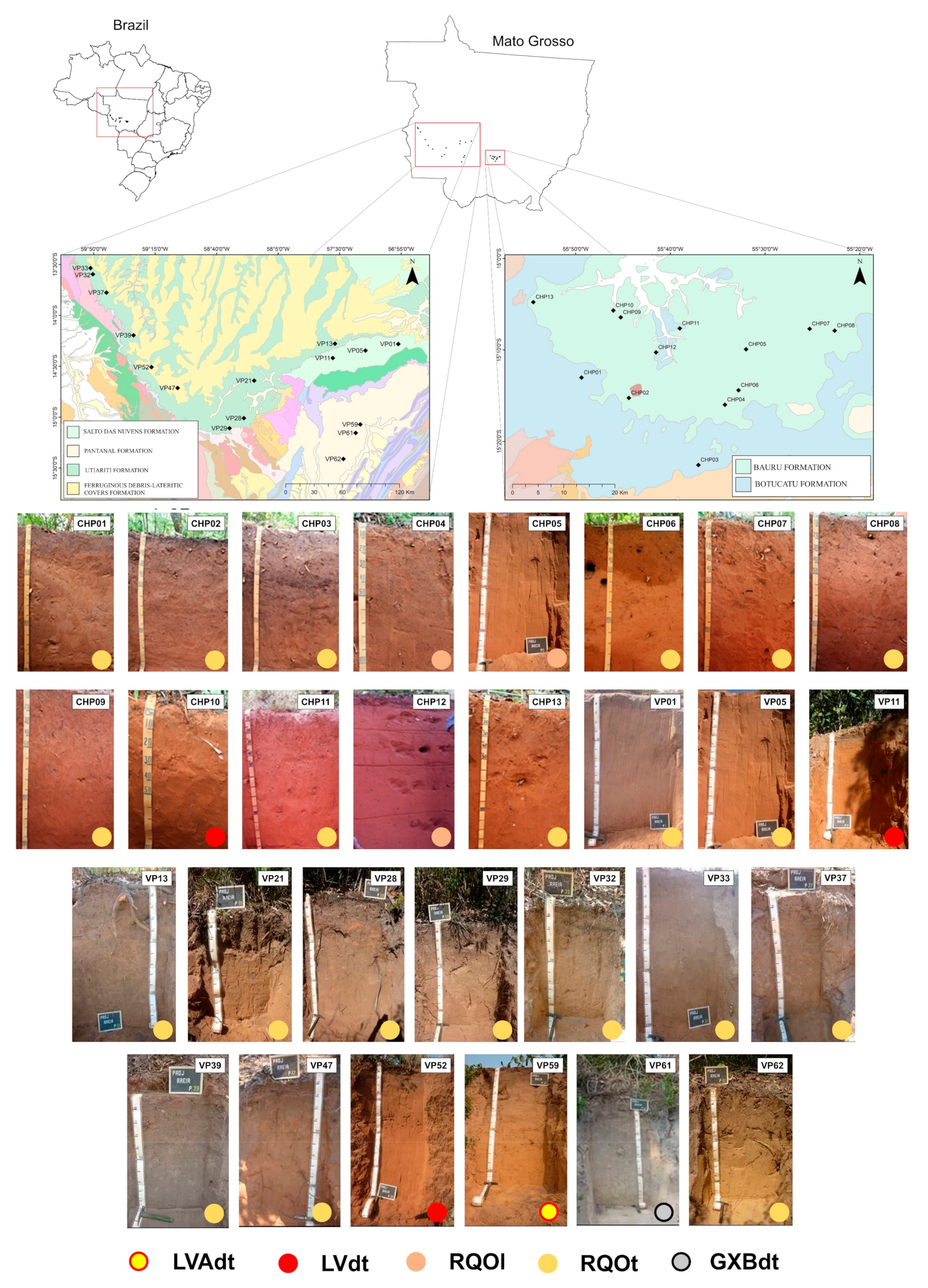
The soil classes identified in the present study, according to the SiBCS, were as follows: RQOt, RQOl, LVdt, LVAdt, and GXBdt.

Fluvisols, Leptosols, Regosols, and Arenosols are known for not presenting significant alterations of the parent material either due to the low intensity of action from the climate, relief, and/or weather factors or due to the high resistance of the parent material itself [2,33,34]. To be classified as Hydrophobic Dystric Arenosol (RQOt), the soil must have a mineralogical composition essentially composed of quartz, not fit into the large group of “hydromorphic”, not have lithic contact up to 150 cm from the surface, and, up to that same depth, have sand loam or loamy sand texture. If the soil, up to 150 cm from the surface, present a morphology similar to Ferralsols with medium texture, caused by a higher content of clay mineral, but with sand loam texture or loamy sand and poor structural development (very small granule), it can be put in the “latossolic” subgroup. Hydrophobic Dystric Arenosol that do not fit morphologically and texturally in the “latossolic” subgroup or any other subgroup are put in the “typical” subgroup.

Ferralsols are known for having a latossolic B horizon up to 200 cm from the surface. This horizon shows an advanced stage of weathering and is mainly composed by resistant to weathering minerals, such as iron, aluminum oxides, quartz, and 1:1 clay minerals [2,33]. The distinction between the suborders of Latosols is mainly a function of the color of the A and B surface horizons. Soils with a hue of 2.5YR or redder in the first 100 cm of the B horizon are categorized in the “red” suborder. Ferralsols that do not fit under the “bruno” or “yellow” suborders will necessarily be categorized as “red-yellow”. It is known that soil color is directly related to its clay mineral content, such as the proportions of hematite and goethite.

Gleysols are characterized by the existence of the gley horizon in the subsurface or, eventually, in the surface. The gley horizon has neutral coloration caused by the reduction of amorphous and crystalline iron present in the soil. Arenic Dystric Gleysol (GXBdt) are Gleysols that do not have sulfidic, histic, or salic horizons; clay with low activity; and base saturation lower than 50% both in most of the B and/or C horizons.

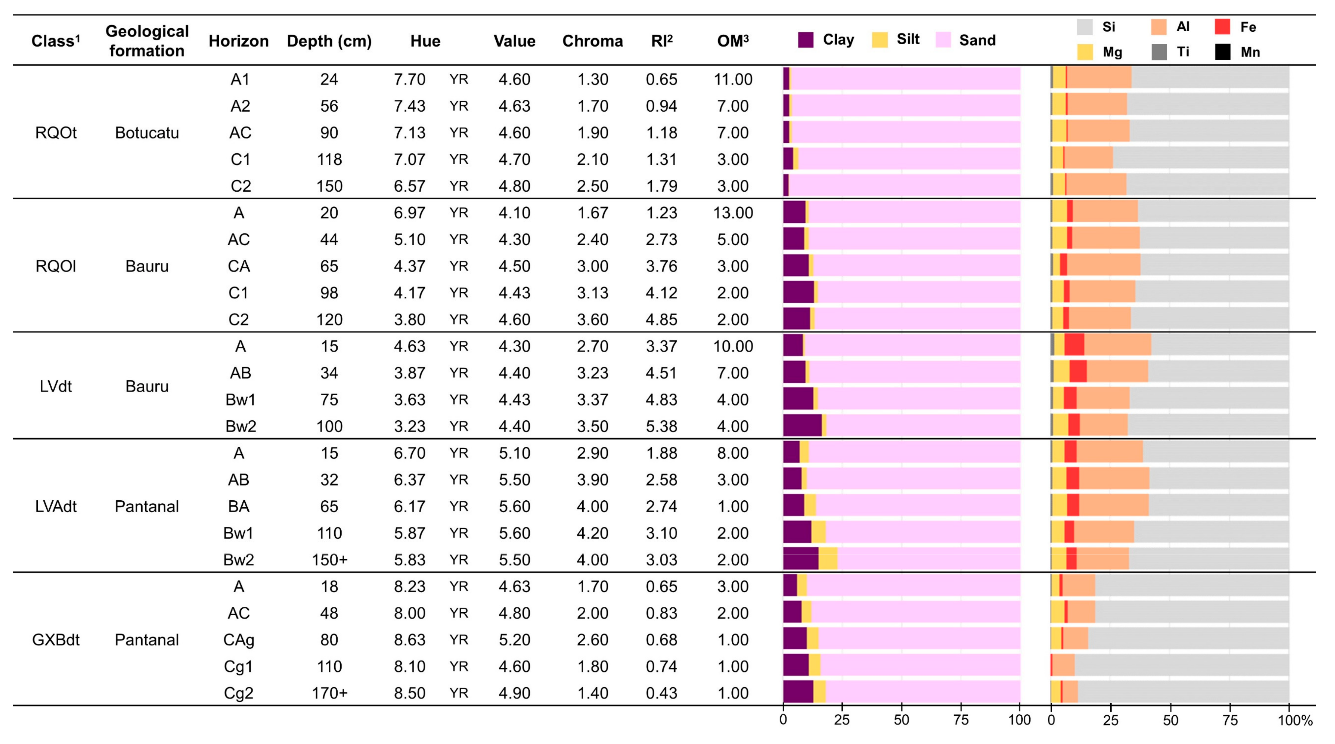
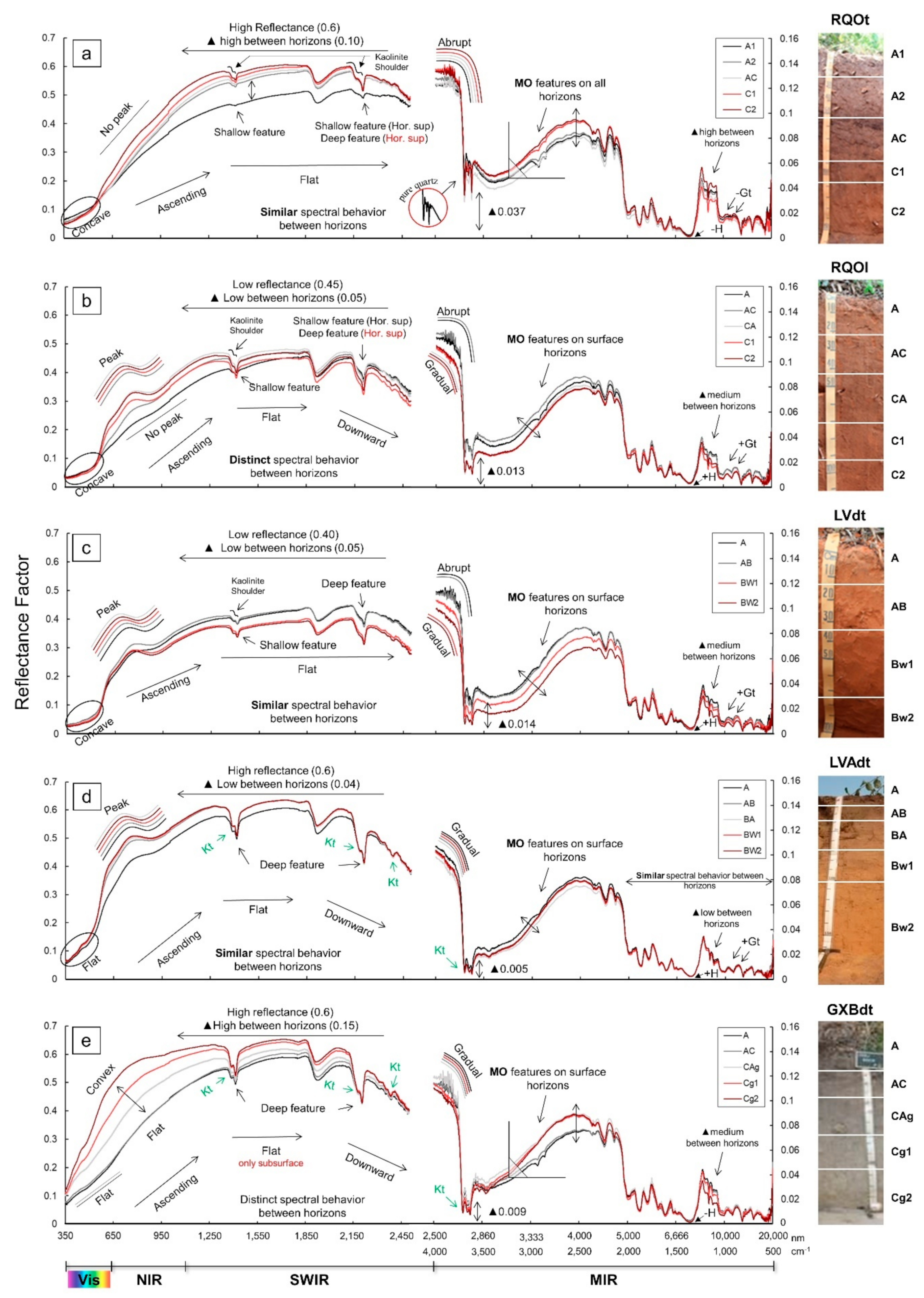
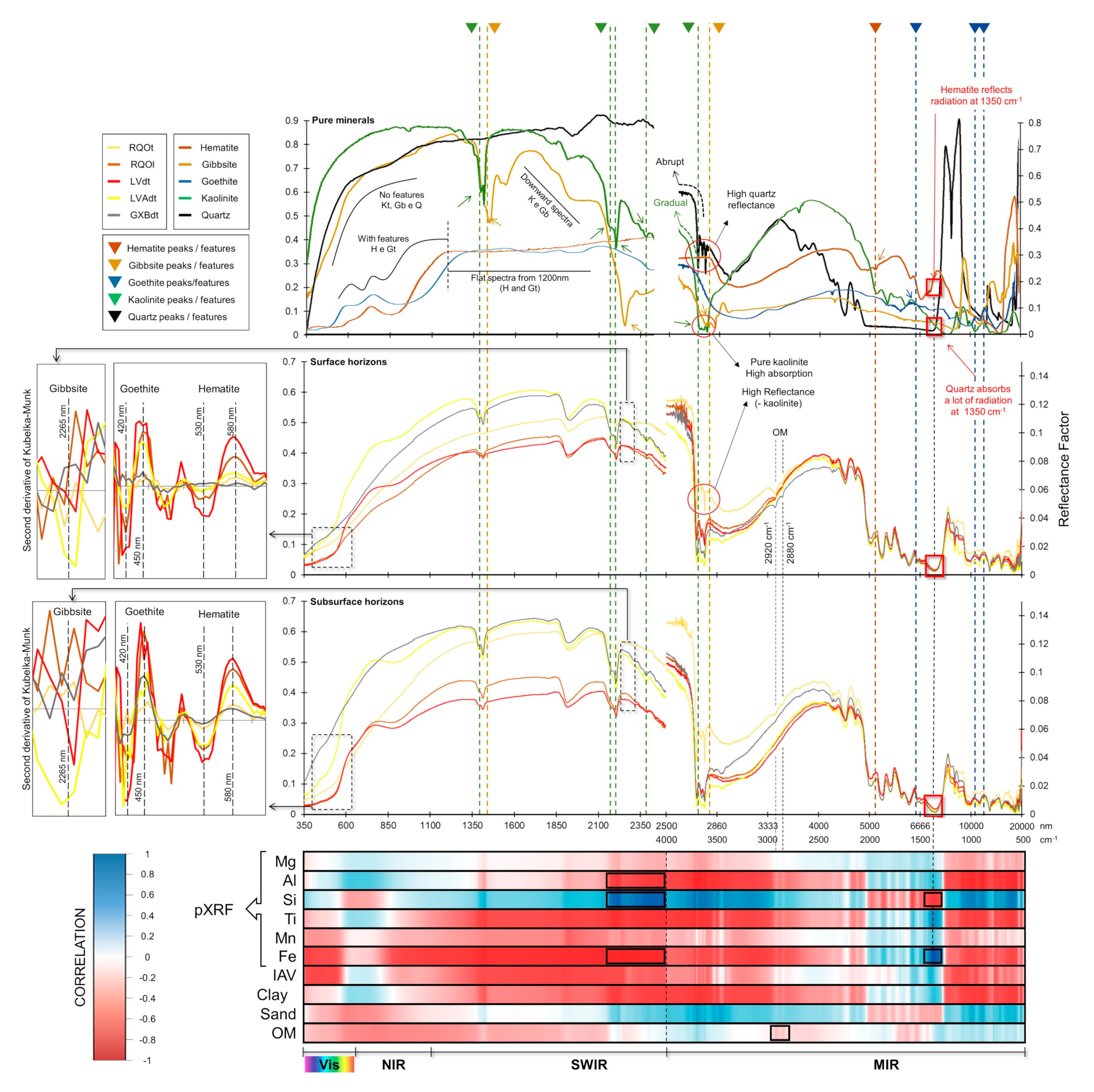
Figure 2 shows the attribute values in each horizon of the identified pedological classes. Figure 3 shows the spectra of the five representative profiles of the soil classes covered by this study. Figure 4 shows the average spectra of surface horizons, subsurface diagnostics of the representative profiles, their second derivative of Kubelka–Munk (KM), correlations with soil attributes and total elemental contents (pXRF), and spectral curves of pure minerals.

The RQOt profile (Figure 3a) showed high reflectance intensity in VNS for all described horizons (0.5 to 0.6). The horizons presented ascending shapes up to 1250 nm and, subsequently, a flat pattern. Ref [5] observed the same patterns in a Hydrophobic Dystric Arenosol from Três Lagoas, MG. It is possible to observe a large variation in reflectance intensity between the subsurface horizons and the A horizon, which is due to the joint action of high sand and OM contents (Figure 2). The high sand content provides a low specific surface [35] that helps to cap sand particles with OM, blur the quartz, and decrease the curve’s general reflectance [9].

Despite the differences in reflectance intensity between the A horizon and the subsurface ones, spectral curves with extremely similar shapes and features were found in the RQOt (Figure 3a). Small exceptions occur in features at 1400, 1900, and 2220 nm of the A horizon, which are shallower as a result of the high OM content (Figure 2) [5,30]. The light concavity found between 350 and 600 nm indicates, at first, low levels of iron oxides in the RQOt profile. The second derivative of KM (Figure 4), calculated for this same interval, confirms the reduced levels of goethite based on the analysis of the peak centralized at 420 nm, and of hematite, whose feature is at 530 nm and peak at 580 nm [10,32].

The KM derivatives at 2265 nm (Figure 4) indicate low gibbsite content in the RQOt profile. The shoulder on the left identified in the 1400 and 2200 nm features, along with the high total Al and Si contents found by pXRF (Figure 2), indicate the presence of kaolinite [9,10,30].

As described by [36], the overlapping of mineral features hardens the characterization of soils through their spectra, as is the case of pure gibbsite and kaolinite features, and the flat pattern of pure quartz close to 1400 and 2200 nm (Figure 4). In sandy soils with high quartz content, this mineral causes high reflectance and the absence of features in the entire spectrum. At around 1400 and 2200 nm, the gibbsite only deepens the feature, and the kaolinite, in addition to deepening, also acts on the formation of shoulders (Figure 4). Thus, in this balance of opposing forces, soils rich in quartz, moderate kaolinite, and low on gibbsite show shallow features, but with the characteristic shoulders at 1400 and 2200 nm. The 2200 nm feature, in the RQOt profile, is deeper than at 1400 nm (Figure 3a), because, at 2200 nm, kaolinite absorbs more radiation (Figure 4), making the feature, in the balance of forces, tend more towards deepening than the flat aspect typical of quartz.

The MIR spectra of the sandy soil profiles did not show differences in the general reflectance intensity of the curves. The differences in the MIR spectra occurred only between horizons and at specific points in the spectrum, coinciding with features and peaks. This is due to microscopic interactions caused by fundamental molecular vibrations in the MIR that produces fundamental features of mineral and organic elements, while in the VNS, “overtones” and combinations predominate [36].

The MIR spectra of the RQOt profile (Figure 3a) showed similar shapes among themselves, as well as the VNS spectra. Notable differences were found in the 2920 and 2880 cm⁻¹ features, in which elongations of OM alkyl-CH₂ groups act with strong influence [37]. The bands centered at 2920 and 2880 cm⁻¹ are deeper in the surface horizons, which have higher OM content, and are shallower in the subsurface horizons, which is due to the inversely proportional relationships between OM and reflectance, as highlighted in the correlation bars in Figure 4. Despite the RQOt profile having a lower OM content in the A horizon than RQOl, for instance, RQOt had deeper features that are certainly due to the higher sand content and, consequently, the smaller contact surface of the particles allows for the low OM content to act with more intensity.

Refs [38,39] report hematite peaks close to 910 cm⁻¹ in MIR spectra. However, this region did not show variations consistent with the low hematite content expected for the RQOt profile, in comparison with the other profiles, based on the iron content of the pXRF analysis and the results obtained with the KM derivatives (Figure 2 and Figure 4).

Analyzing the MIR spectra of pure quartz and hematite and comparing them with the spectra of the RQOt profile, we can identify another region sensitive to hematite (Figure 4). At 1350 cm⁻¹, quartz absorbs all the radiation, while hematite reflects most of the incident radiation. Thus, sandy soils with low hematite content and high quartz content will tend to show high absorption at 1350 cm⁻¹. The higher the hematite content, the higher the reflectance in this region. This statement can be confirmed by analyzing the radiation absorbed by the RQOt at 1350 cm⁻¹, and comparing it with RQOl and LVdt, which are the profiles with the highest hematite content. Furthermore, in the correlation analysis, shown in Figure 4, it is noted that the region near the 1350 cm⁻¹ feature shows a high correlation with Si (−0.70) and with Fe (+0.85), confirming the sensitivity of this region for identifying hematite in sandy soils.

According to [8], gibbsite and kaolinite features happen near 3500 cm⁻¹ in MIR spectra. This characteristic can also be found in the spectra of these pure minerals (Figure 4). Unlike the VNS spectra, MIR could not identify the features of gibbsite and kaolinite due to the superposition of the characteristic features of these minerals with strong quartz features between 3690 and 3620 cm⁻¹ (Figure 4). In this region, quartz reflects a lot of radiation, while gibbsite and goethite do the opposite. The content of these minerals was not enough to express features in this region, since the RQOt profile has high contents of sand and quartz (Figure 2). Furthermore, it is noted that in the initial portion of the MIR spectrum, from 4000 to 3700 cm⁻¹, the high quartz content conditioned the abrupt pattern (Figure 3a), characteristic of pure quartz (Figure 4). The high contents of sand and quartz of the RQOt profile are also evident between 1300 and 1000 cm⁻¹ due to the asymmetric vibrations of Si-O-Si that manifest two characteristic peaks (Figure 3a).

From the different findings made in the VNS and MIR spectra of the RQOt profile, it is concluded that the combination of high reflectance intensity; characteristics of high contents of sand and quartz; the similarity between the spectral curves of the horizons; absence of typical features, or poor expressions that indicate reduced levels of hematite, goethite, and gibbsite; and presence of kaolinite in small amounts are indications that induce its inclusion in the class of RQOt.

The RQOl profile (Figure 3b) showed low reflectance intensity and small amplitude of variation between horizons in VNS (0.40 to 0.45). Different from the pattern found in the RQOt, the RQOl profile manifested an ascending shape up to 1250 nm, a flat shape up to 2200, and, subsequently, a downward tendency. These different shapes in the curves among profiles are due to variations in clay content. This pattern is due to the great influence that quartz has on the reflectance intensity in VNS, especially in SWIR [15]. Thus, small increases in the clay content of sandy soils tend to show downward patterns after 2200 nm. Ref [9] also found that increases in clay content provide a downward aspect in the final section of the spectrum of sandy soil. In Figure 4, we can see a directly proportional correlation between Si and reflectance in this region, with r values always greater than 0.8. In this same spectral region, Al and Fe, which are oxide elements that generally compose the clay fraction of tropical soils, have an inversely proportional relation with reflectance values, with correlations from −0.6 to −0.8 and −0.8 to −1, respectively.

The A horizon of the RQOl profile showed softer features around 800, 1400, 1900, and 2200 nm than the other profiles due to its high OM content [5,9]. OM contents close to 17 g kg⁻¹ can mask iron oxide features, which is even more intensified in soils with low levels of these oxides [9,40]. The RQOl profile showed higher contents of hematite and goethite than RQOt, which can be visibly identified in the peaks between 650 and 950 nm and the stronger concavities between 350 and 650 nm (Figure 3b). These findings are confirmed by analyzing KM derivatives (Figure 4) and total Fe contents (Figure 2). The analysis of the gibbsite, which was carried out for the RQOl profile from the KM derivative at 2265 nm (Figure 4) and the shallow feature at 1400 nm with a shoulder on the left wall of the valley, indicate a lower content of gibbsite than kaolinite.

The MIR spectra of the RQOl profile (Figure 3b) showed similar shapes among themselves, with notable features in the 2920 and 2880 cm⁻¹ bands in the A horizon and soft features in the AC horizon, caused by OM. The highest levels of hematite can also be found in the MIR spectra of the RQOl profile, in the region near 1350 cm⁻¹, where the curves are further away from the X-axis. Goethite features, at 960 and 880 cm⁻¹ of the pure spectrum of this mineral (Figure 4), can be seen in the MIR spectra of the RQOl profile (Figure 3b), which agrees with the results from the KM derivative of this profile. These same features cannot be seen in the MIR spectra of the RQOt profile (Figure 3a) since it has a low content of goethite.

Another difference between the MIR spectra of the RQOl and RQOt profiles is the kaolinite features between 3700 and 3600 cm⁻¹. In RQOl, these features are sharper and closer to the X-axis, showing the kaolinite absorption pattern in this region. Possibly, the more evident manifestation of kaolinite features in the MIR spectrum of the RQOl profile than the RQOt was due not only to its higher kaolinite content but also due to the lower contents of sand and quartz in this profile (Figure 2), which decrease the masking effect. The subsurface horizons showed higher kaolinite content. In the initial portion of the RQOl MIR spectra, we saw gradual patterns for the subsurface horizons, where kaolinite showed a feature with great intensity, and abrupt patterns for the surface horizons. The lower quartz contents in RQOl can also be seen by the reduction of double peak intensities at 1300 and 1000 cm⁻¹.

Pedologically, the RQOl profile (Figure 3b) differs subtly from the RQOt profile (Figure 3a), as it is included in the “latosolic” subgroup [2]. This subtle pedological distinction can be identified by pedometry using descriptive analyses of VNS and MIR spectra that show the highest contents of hematite, goethite, and kaolinite in RQOl.

The LVdt profile (Figure 3c) showed, in VNS, the lowest reflectance intensity among the studied profiles (0.35 to 0.40) and great similarity of features between horizons. The spectral curves showed ascending shapes up to 1200 nm that remained flat after. The combination of low reflectance intensity and flat shape from 1200 nm in the LVdt profile is due to its high iron oxide content (hematite and goethite) found in the KM derivatives (Figure 4) and represented in the pXRF analysis (Figure 2). Refs [5,30,41] also identified flat shapes in VNS starting at 1200 nm for LVdt rich in hematite and goethite. It is important to emphasize that the combination of flat shapes and low reflectance intensity, found in LVdt, differs from the combination of flat shape and high reflectance intensity of RQOt, which is due to high quartz content and, consequently, the reflectance pattern of this mineral is seen in its pure spectrum (Figure 4).

A pattern distinct from the others was observed in the VNS spectra of the LVdt profile, since the A and AB surface horizons had higher reflectance intensities than the Bw1 and Bw2 subsurface horizons. This pattern was due to the higher clay content found in the Bw horizons that provided a textural B/A ratio of 1.42. Thus, even the high OM content, observed in the A and AB horizons, was not enough to have lower reflectance intensity than the underlying ones (Bw1 and Bw2). Ref [5], studying a typical dystrophic Red Latosol with medium texture, observed the lowest reflectance intensities in the A horizon. However, the textural B/A ratio found by these authors was 1, which made the high OM content on the surface the determining factor for the inversion of reflectance intensity. Unlike what was noted for the RQOl profile, the A horizon of the LVdt profile showed sharp hematite features between 650 and 950 nm. Beyond showing hematite and goethite, the VNS spectra of the Bw horizons of the LVdt profile indicate the presence of gibbsite, according to the KM derivatives (Figure 4), and kaolinite, due to the presence of a shoulder in the 1400 nm feature and deeper feature at 2200 nm.

Despite demonstrating sensitivity for identifying hematite, goethite, and kaolinite, the MIR spectra of the LVdt profile (Figure 3c) were very similar to the RQOl profile. The only differences found were: (I) the more discrete OM features in the 2920 and 2880 cm⁻¹ bands of the A horizon possibly overshadowed by the higher levels of iron oxides in LVdt (Figure 2); (II) the differences in reflectance intensity between 3600 and 2000 cm⁻¹ provided by clay increments in the LVdt subsurface horizons. Although MIR’s high sensitivity for identifying minerals in the soil, evidenced many times in several renowned studies [8,42], the few variations found here are not enough to differentiate the RQOl and LVdt sandy profiles. However, despite the inefficiency of the MIR for this specific case, the VNS spectra showed great distinction potential, as they were sensitive to the higher contents of iron oxides and kaolinite found in LVdt and showed very distinct patterns of reflectance intensity and shape of curves in comparison with RQOl.

The VNS spectra of the LVAdt profile (Figure 3d) showed high reflectance intensities that are comparable to the ones from RQOt (Figure 3a) and much higher than LVdt and RQOl (Figure 3b,c), even though LVAdt had a higher clay content. The LVAdt spectra are extremely similar. Different from LVdt, this profile showed lower reflectance intensity in the A horizon, even with the addition of subsurface clay (Figure 2), and shapes with an ascending aspect up to 1200 nm, flat between 1200 and 2200 nm, and downward from then on. The high reflectance intensity and shape of the curves in LVAdt are due to the predominant clay minerals in its constitution.

Different from the LVdt profile, the LVAdt profile shows a predominance of kaolinite and gibbsite, which can be seen in the KM derivatives (Figure 4) and the very striking characteristic features at 1400, 2200 (shoulders), and 2400 nm (Figure 3d), respectively [9,10,30]. The higher contents of gibbsite and kaolinite found for the LVAdt profile justify the differences in shapes and reflectance intensity in comparison to the LVdt, in which the hematite and goethite predominate. According to the spectra of pure minerals (Figure 4) for VNS, it is observed that kaolinite and gibbsite show high reflectance intensities with a strong downward pattern starting at 2200 nm. These patterns, observed for kaolinite and gibbsite, are quite different from the ones observed for hematite and goethite, which absorb much of the incident radiation and manifest a practically flat shape throughout the VNS. From the KM derivative, it was noted that the LVAdt profile has a higher proportion of goethite than hematite (Figure 4), justifying its inclusion in the “Red-Yellow” group. Ref [5] analyzed a typical dystrophic LVAdt profile from the region of Lagoa da Prata (MG) with 350 g kg⁻¹ of sand and 630 g kg⁻¹ clay, and aluminum oxide contents (26.29 g kg⁻¹) three times greater than iron oxides (9.11 g kg⁻¹). In this scenario, the authors found patterns of spectral behavior very similar to the ones obtained for the LVAdt profile (Figure 3d), differing only in terms of reflectance intensity, as a function of the sandy texture of the profile characterized in this study.

The LVAdt’s MIR spectra (Figure 3d) show extremely similar shapes among themselves, with small differences in reflectance intensity between 4000 and 2250 cm⁻¹ and notable OM features in the A horizon. The high contents of gibbsite and kaolinite throughout the LVAdt profile are seen by the gradual patterns at the beginning of the spectra and in the sharp features with high absorptions between 3700 and 3500 cm⁻¹.

The pure spectra of kaolinite and gibbsite show gradual patterns at their beginnings (4000 to 3700 cm⁻¹), while hematite, goethite, and quartz show abrupt patterns (Figure 4). LVAdt has high contents of gibbsite and kaolinite in all horizons, according to KM derivatives (Figure 4), and features between 3700 and 3500 cm⁻¹ that show gradual patterns throughout the profile (Figure 3d). Comparatively, it is also noted by KM derivatives and features between 3700 and 3500 cm⁻¹ that there are increases in the gibbsite and kaolinite contents in the LVdt subsurface horizons, precisely where the gradual patterns manifested themselves (Figure 3c).

In the LVdt surface horizons, where hematite, goethite, and quartz are predominant, the abrupt patterns are manifested. Again, the reflectance intensity around 1350 cm⁻¹ was coherent with variations in the hematite content, since the interval between the X-axis and the valley of the feature at this wavelength in LVAdt was bigger than in RQOt and GXBdt and lower than in RQOl and LVdt. Despite having no notable difference in shape between LVAdt and LVdt in the MIR spectra, as in VNS, mineralogical differences between these classes at specific points in the spectra were identified.

The VNS spectra of the GXBdt profile (Figure 3e) showed high reflectance intensities and a large range of variation between horizons, following exactly the patterns found by [5,9,43,44]. The gley ACg, Cg1, and Cg2 horizons did not show concavities caused by iron oxides between 850 and 900 nm and showed a convex pattern between 350 and 1250 nm.

In the A and AC surface horizons, in which no gleyzation processes were identified, the spectra format was similar to the ones observed for RQOt, since both have low contents of hematite and goethite and high content of quartz (Figure 3a,e). This finding highlights the importance of evaluating all horizons for the characterization and classification of soil profiles by spectroscopy. The GXBdt profile showed low contents of iron oxides and gibbsite, according to the KM derivatives (Figure 4) and the pXRF analysis (Figure 2). However, the typical features at 1400, 2200 (shoulders), and 2400 nm and the shape of the curves, with ascending, flat, and descending aspects, indicate a predominantly kaolinitic mineralogical constitution. The kaolinitic constitution theory of this profile can also be reinforced by the pXRF analysis of total elements, which indicated the predominance of Al and Si.

Different from what was seen in VNS, the MIR spectra of the GXBdt profile did not have shapes or features that typically would characterize a Gleysol, a fact also found by [44]. However, it was possible to identify patterns that characterize the presence of kaolinite, with typical features and high absorption between 3700 and 3500 cm⁻¹, and absence of hematite, with high absorption in the 1350 cm⁻¹ feature.

Between 3000 and 2225 cm⁻¹ from the GXBdt profile, inclination changes were noted between the curves of the surface and subsurface horizons (Figure 3e). This may be due to the low content of iron oxides (hematite and goethite) in this profile that makes the contrast of OM between surface and subsurface a determining distinction factor. Thus, in the superficial horizons, OM changes the inclination between 3000 and 2225 cm⁻¹, where elongations of alkyl-CH₂ groups act with a strong influence [37]. Meanwhile, quartz, which is more exposed in the subsurface where the OM content is lower, induces increases in reflectance and an ascending pattern in this region, as shown by its pure spectrum (Figure 4). This action of opposing forces causes this region to have a slight difference in inclination between the surface and subsurface horizons. This pattern can be seen in the two profiles with almost zero iron oxides, such as GXBdt and RQOt (Figure 3a,e). However, in the GXBdt profile, the inclination is more pronounced, due to the high quartz content. This profile has a lot of kaolinite, which, according to its pure spectrum (Figure 4), induces a strong ascent in this region, increasing the degree of the inclination.

The VNS region showed a high capacity to differentiate sandy soil classes using the MIRS concept to interpret the spectra of the profiles studied here. The RQOt profile showed spectral characteristics in agreement with [5] and completely different from the RQOl. RQOl showed differences in shape, intensity, and mineralogical constitution in comparison with LVdt. The LVAdt profile showed patterns in agreement with [5,10]. Despite also being included in the order of Latosols and having a high sand content, LVAdt was quite different from LVdt. The GXB profile showed patterns characteristic of the order of Gleysols, which is completely different from the other profiles studied.

The application of the MIRS concept in the MIR spectra was not effective for distinguishing the sandy soil classes studied here since they do not show notable patterns of distinction in the general shape of the curves and reflectance intensities. Ref [44] also noted MIR’s low capacity to manifest patterns of distinctive spectral behavior across soil classes. This is due to the fundamental molecular vibrations in the MIR that manifest alterations in very specific places in the spectrum, but with little influence on the general shape and reflectance intensity of the curves. However, this region proved to be very important for the identification of mineralogical constitution, texture, and OM contents between the soil classes and their respective profiles. Thus, despite not being applicable for class distinction, the MIR region has great importance for the complementation of soil pedometric characterizations using VNS spectroscopy. Additionally, here, we highlight the great importance of the joint analysis of different information obtained by remote sensors, such as VNS, MIR, and pXRF, which, even with their specificities, allow pedologically complex characterizations and conclusions in a short period and with low investment in analysis and reagents.

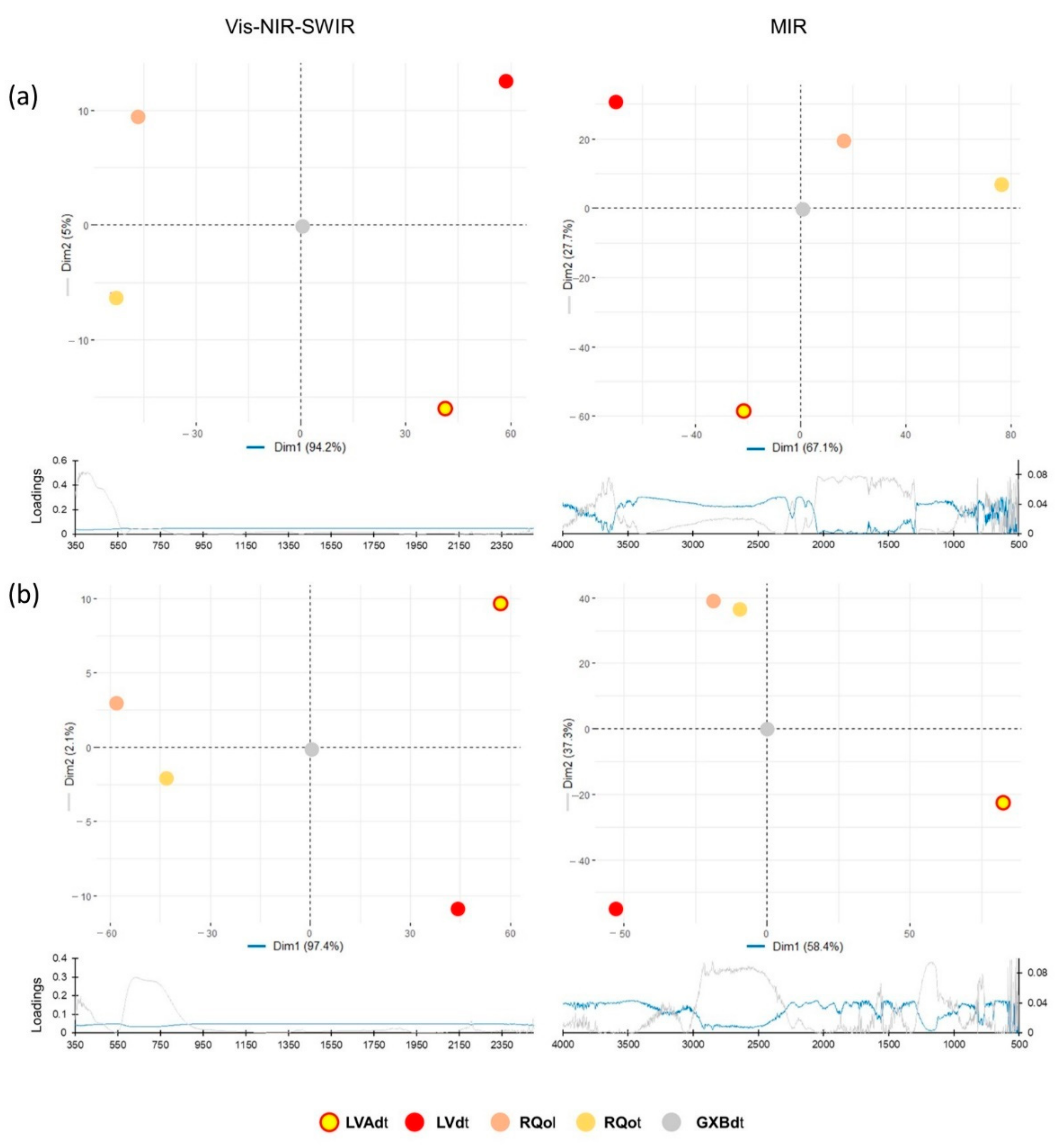
The PCA’s, done with the VNS spectra, showed a high capacity for distinguishing soil classes, both on the surface (Figure 5a) and subsurface (Figure 5b), and were in agreement with the MIRS method of visual characterization. Dimension 1 of the VNS PCA’s presented a contribution of 94.2%, on the surface, and 97.4%, on the subsurface, and was able to distinguish the profiles: Ferralsols (LVdt and LVAdt), Arenosols (RQOt and RQOl), and Gleysol (GXBdt). Dimension 2 had contributions of only 5% and 2.1% but allowed for distinctions between the subgroups of Arenosols, típico (RQOt) and latossólico (RQOl), and between the Ferralsols (LVdt and LVAdt) suborders of the Ferralsols. Analyzing the loadings of dimension 2 of the PCA’s VNS, the contribution peaks are between 350 and 950 nm. These peaks are exactly where the hematite and goethite peaks are manifested, and they are responsible for the distinctions between LVdt and LVAdt, and between RQOt and RQOl.

As in the MIRS analysis of visual characterization, the MIR spectra performed worse than VNS for distinguishing soil profiles. At the surface, dimension 1, which had a contribution of 67.1%, was able to distinguish Ferralsols from RQOt and RQOl; however, the Gleysol did not show a clear distinction from the others (Figure 5a), possibly due to the absence of gley characteristics in the horizons A and Ac of this profile.

Dimension 2 of the surface PCA only distinguished the LVAdt from the others. In the subsurface, dimension 2, which had a contribution of 37.3%, was able to distinguish Ferralsols, Arenosols, and Gleysol (Figure 5b). The distinction between the suborders of Latosols can be seen in dimension 1. The PCA’s elaborated from the MIR spectra showed a low ability to distinguish RQOt and RQOl at the level of suborders, both on the surface and the subsurface.

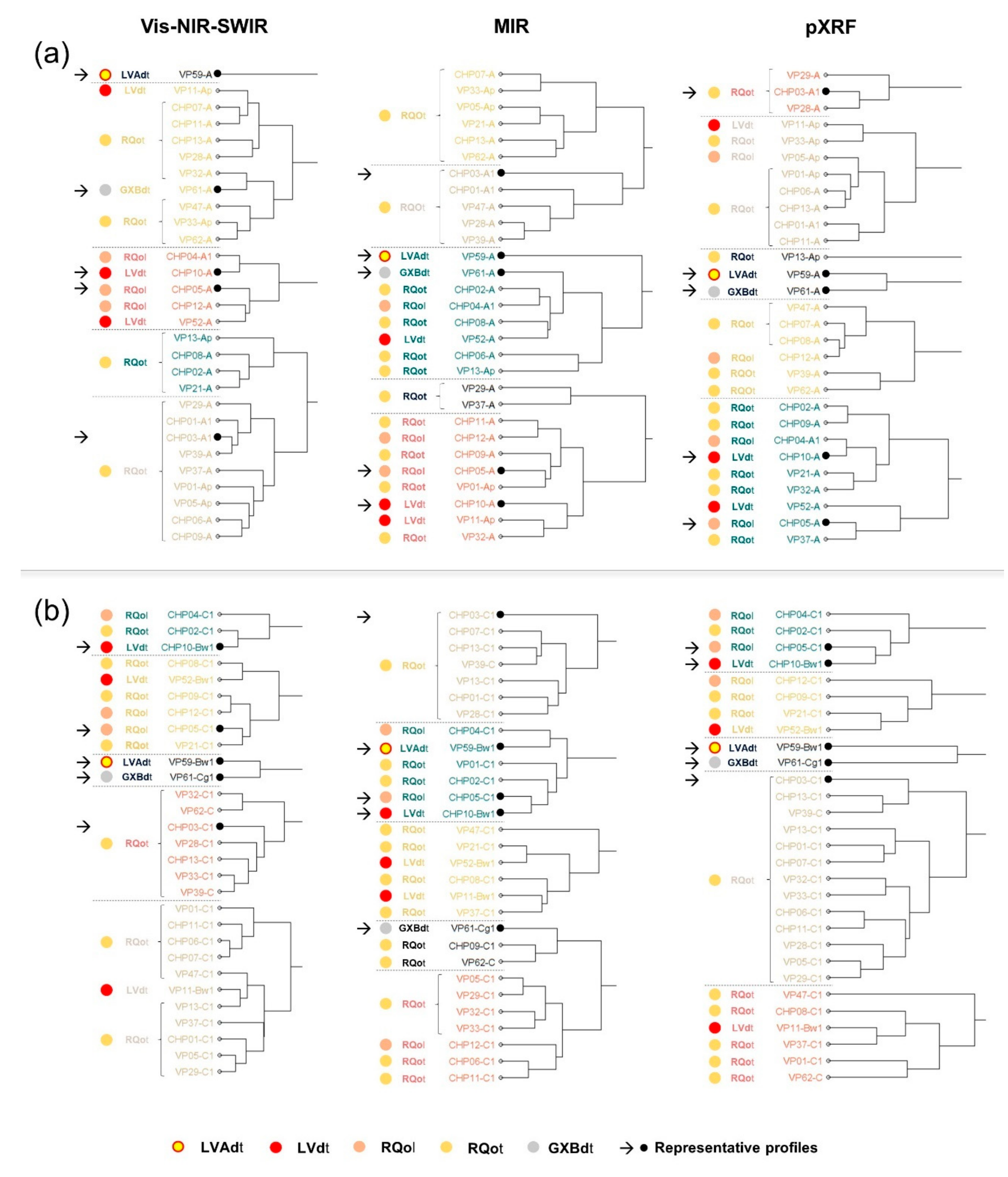
Figure 6 shows the distribution of the 29 profiles described in this study, clustered into five groups based on surface and subsurface data (first layer of the diagnostic horizon). The clusters showed a reasonable ability to distinguish representative profiles (→●). The performances of the predictor variables of clustering were, from best to worst: VNS, MIR, and pXRF. The PCA technique was more effective than the cluster technique to distinguish representative profiles.

Another important factor to be analyzed is that clusterings did not provide convincing groupings when including the other profiles. This is due to the tenuous limits that distinguish the sandy soil classes analyzed in this study. In other words, even profiles included in the same class may present variations in chemical, physical, and mineralogical attributes among themselves, inducing small overlapping patterns and, consequently, making the limit of distinction between classes unreachable for “machine learning”. For example, pedologically, when ranking sandy soils classified as RQOt, RQOl, and LVdt, it is considered that (I) the soils with the lowest clay mineral contents, mainly hematite, and goethite, will be classified as RQOt; (II) as clay mineral contents increase, even within the RQOt classes, there will be a tenuous limit in which morphological changes (soil structures or aggregates) will be noticeable and, at this point, the analyzed profile will no longer be an RQOt and will be classified as RQOl; (III) in the same way if the clay mineral contents continue to increase to a certain limit, the RQOl class tends to LVdt.

Refs [10,30] found excellent capabilities for grouping different soil classes using clusters. However, despite the great advances provided by these studies, the profiles analyzed by them were very different from each other, in terms of texture, mineralogy, and source materials. However, differently from the studies of the mentioned authors, in the present study, the “machine learning” techniques alone did not work well to distinguish extremely similar sandy soils. Ref [41] concluded that cluster analysis along with descriptive analysis proved to be adequate for the discrimination of soil types, reinforcing the importance of human reflections.

The present findings of clustering using spectra do not reduce the potential for using remote sensing techniques, and quite the opposite, they only reinforce that human decision-making power is of great importance for soil classification, but it can and should be optimized by technologies. Hence, remote sensing presents itself as a support tool to integrate information, reduce subjectivity, and, consequently, help the decision-making capacity of pedologists around the world. In agreement with the results obtained here, ref [19] concluded that remote sensing techniques alone reduce the subjectivity of pedological interpretations, but do not replace the mental and interpretative process.

This descriptive analysis of spectra demonstrated the potential of proximal sensing for the characterization of sandy soils and, consequently, their distinction. Works with the same objective may contribute to a better categorization of sandy soils around the globe, characterizing production environments in a more accurate way.

3.2. Modeling Sandy Soil Attributes

Soil characterizations, whether for pedological or agronomic purposes, require a lot of analysis since some soil attributes cannot be obtained in the field with a certainty level sufficiently safe. Therefore, it is paramount to evaluate the capacity of spectroscopy, in the VNS and MIR regions, and X-ray fluorescence analysis in determining the physical and chemical attributes of sandy soils. The use of these technologies optimizes soil characterization, reduces cost, and, also, excludes the need for chemical reagents that are potentially harmful to the environment if managed incorrectly.

Table 1. Parameters from mathematical models for estimating soil attributes based on Vis-NIR-SWIR, MIR, and pXRF data (Cal: calibration; Val: validation; VNS: Vis-NIR-SIWR; R²: coefficient of determination; RMSE: root means error square; RPIQ: ratio of performance to interquartile distance; VFS, very fine sand; FS, fine sand; MS, average sand; CS, coarse sand; PLSR: “Partial Least Square Regression”; RF: “Random Forest”).

Attribute	Joint	VNS				MIR				pXRF				VNS + MIR				VNS + MIR + pXRF
		Model	R2	RMSE (%)	RPIQ	Model	R2	RMSE (%)	RPIQ	Model	R2	RMSE (%)	RPIQ	Model	R2	RMSE (%)	RPIQ	Model	R2	RMSE (%)	RPIQ
Hue	Cal	Cubist	0.98	2.53	13.60	Cubist	0.87	7.60	4.12	Cubist	0.75	9.93	3.32	Cubist	0.98	2.74	11.93	Cubist	0.97	3.14	10.71
	Val		0.97	3.75	9.00		0.76	10.95	3.40		0.47	14.19	2.23		0.93	4.97	6.35		0.95	4.46	7.48
Value	Cal	Cubist	0.80	2.58	2.00	PLSR	0.61	3.48	1.31	Cubist	0.68	3.79	1.19	Cubist	0.84	2.58	1.75	Cubist	0.78	2.73	1.66
	Val		0.74	3.03	1.53		0.28	4.85	0.95		0.31	3.64	0.98		0.74	2.88	1.22		0.66	3.03	1.28
Chroma	Cal	Cubist	0.96	3.81	7.21	PLSR	0.87	6.43	4.2	Cubist	0.66	10.71	2.67	Cubist	0.95	4.05	6.15	Cubist	0.93	4.76	5.83
	Val		0.84	7.38	3.45		0.79	9.05	3.45		0.45	13.10	2.10		0.92	5.24	5.42		0.88	5.95	4.22
RI	Cal	Cubist	0.99	2.75	14.17	Cubist	0.92	8.89	5.21	PLSR	0.70	14.23	2.75	Cubist	0.99	3.07	12.74	Cubist	0.99	2.91	13.30
	Val		0.96	5.98	7.90		0.72	12.93	2.85		0.58	19.72	2.42		0.94	6.79	7.58		0.94	6.95	6.84
Clay	Cal	Cubist	0.81	8.33	3.17	PLSR	0.67	9.54	2.86	RF	0.50	11.51	2.13	PLSR	0.96	3.36	6.71	PLSR	0.85	6.58	3.54
	Val		0.57	9.71	1.46		0.63	11.07	1.23		0.40	10.31	1.47		0.64	9.30	2.12		0.64	10.38	1.94
Silt	Cal	Cubist	0.88	9.88	4.82	PLSR	0.93	7.38	6.48	Cubist	0.68	15.76	3.06	PLSR	0.79	13.00	3.50	PLSR	0.95	6.00	7.96
	Val		0.43	20.00	2.25		0.64	12.38	2.49		0.61	17.05	2.43		0.64	16.00	3.06		0.64	18.38	2.37
Total Sand	Cal	PLSR	0.71	1.71	2.43	PLSR	0.60	2.42	1.78	Cubist	0.56	2.58	1.43	PLSR	0.89	1.07	3.48	PLSR	0.80	1.62	2.97
	Val		0.65	3.12	1.9		0.60	2.11	2.37		0.31	2.76	1.79		0.62	2.47	1.50		0.63	2.30	1.53
VFS	Cal	Cubist	0.79	9.50	3.20	PLSR	0.52	12.69	2.38	Cubist	0.36	15.09	2.02	Cubist	0.84	8.72	3.49	Cubist	0.85	8.46	3.60
	Val		0.59	13.05	2.67		0.49	15.14	2.04		0.40	14.93	2.34		0.78	11.28	3.10		0.77	11.68	2.99
FS	Cal	PLSR	0.98	2.09	11.33	PLSR	0.72	7.78	2.83	Cubist	0.40	12.84	1.88	PLSR	0.95	3.32	6.14	Cubist	0.84	6.06	4.03
	Val		0.65	8.44	2.31		0.61	10.89	2.25		0.17	14.04	1.01		0.68	11.20	2.25		0.65	11.61	1.65
MS	Cal	PLSR	0.89	6.50	4.06	PLSR	0.84	7.21	3.09	RF	0.27	16.92	1.49	PLSR	0.83	7.50	3.35	PLSR	0.91	5.83	4.44
	Val		0.37	16.70	1.34		0.36	20.02	1.49		0.28	17.80	1.74		0.61	14.97	1.82		0.67	12.57	1.81
CS	Cal	PLSR	0.87	8.15	2.34	PLSR	0.80	10.36	1.66	RF	0.14	24.68	0.79	Cubist	0.90	8.26	1.90	PLSR	0.95	5.18	3.62
	Val		0.40	22.04	0.79		0.20	24.46	0.86		0.10	15.43	0.67		0.16	26.77	0.67		0.44	19.72	0.76
pH (H2O)	Cal	PLSR	0.83	1.82	2.97	PLSR	0.97	0.73	7.39	Cubist	0.45	3.09	1.76	PLSR	0.82	2.00	2.73	PLSR	0.69	4.36	3.21
	Val		0.53	2.55	1.93		0.41	4.18	1.32		0.18	3.64	1.24		0.16	3.45	1.55		0.43	6.36	1.88
CTC total	Cal	PLSR	0.83	3.60	3.58	PLSR	0.59	5.34	2.16	Cubist	0.61	8.63	1.41	Cubist	0.57	6.99	1.60	Cubist	0.78	6.99	1.75
	Val		0.38	9.97	1.01		0.58	7.30	1.79		0.10	12.13	1.12		0.20	14.29	1.11		0.08	11.10	0.93
V%	Cal	PLSR	0.69	6.68	2.82	PLSR	0.94	2.93	6.33	RF	0.44	9.04	2.12	PLSR	0.92	3.09	5.37	Cubist	0.93	4.08	3.77
	Val		0.59	7.13	2.55		0.69	6.95	1.86		0.48	6.68	2.20		0.72	6.60	2.65		0.51	2.90	1.82
OM	Cal	PLSR	0.68	7.69	2.00	Cubist	0.62	12.12	1.27	Cubist	0.26	13.62	1.41	PLSR	0.71	8.73	1.87	Cubist	0.77	11.04	1.74
	Val		0.33	11.08	1.73		0.30	20.38	1.13		0.10	21.88	0.79		0.35	12.69	1.51		0.04	15.38	1.25

shows the parameters of the mathematical models obtained for the chemical and physical attributes of the studied soils. For each predicted variable, the best predictive model is highlighted. From the 15 soil attributes modeled, VNS + MIR data showed the best performance for six, VNS for five, MIR for two, and VNS + MIR + pXRF for two (Table 1). PLSR and Cubist stand out among the proposed modeling methods. The pXRF data, used separately, did not have a good predictive performance.

For the attributes related to soil color, the VNS region had a high predictive capacity (Table 1), as expected. For hue, value, and RI, the best models used VNS, with R², RMSE, and RPIQ values of 0.98, 2.53%, and 13.60; 0.80, 2.58%, and 2.00; and 0.74, 3.03, and 1.53, respectively, for calibration; and 0.97, 3.75%, and 9.00; 0.74, 3.03%, and 1.53; and 0.96, 5.98%, and 7.90, respectively, for validation. For chroma, the best mathematical adjustment used VNS + MIR and the values of R², RMSE, and RPIQ were 0.95, 4.05, and 6.15 for calibration and 0.92, 5.24, and 5.42 for validation, respectively. Ref [19] related hue, value, and chroma from soils with texture ranging from sandy to clayey determined by colorimeter, and VNS spectroscopy obtained results inferior to the ones from the present study, with coefficients of determination of 0.88, 0.92, and 0.91, respectively. The authors also analyzed the relationship of these soil color indices obtained by colorimetry and spectroscopy with the traditional method based on interpretations of the Munsell chart. In this analysis, the authors observed a wide range of results, with R² values ranging from 0.20 to 0.86, reaffirming the great subjectivity of traditional analyses and the great potential for incorrect interpretations that result in erroneous soil classifications [45]. Thus, considering that the color is very important to correctly classify soils, spectroscopy techniques have great potential to replace the traditional method even for sandy soils, as shown in the present study. This argument is empowered when considering the speed of execution, independence of reagents, low cost, and, above all, the sheer amount of information that can be obtained from a single spectrum.

For clay content, VNS + MIR had the best predictive capacity with R², RMSE, and RPIQ values of 0.96, 3.36%, and 6.71 for calibration and 0.64, 9.30%, and 2.12 for validation, respectively (Table 1). For the silt fraction, MIR had the best predictive capacity, with R² of 0.93 and 0.64, RMSE of 7.38% and 12.38%, and RPIQ of 6.48 and 2.49, for the calibration and validation clusters, respectively. For total sand, the VNS + MIR combination provided the best predictive models, with R², RMSE, and RPIQ values of 0.89, 1.07%, and 3.48 for calibration and of 0.62, 2.47%, and 1.50 for validation, respectively. The low capacity of pXRF to estimate texture may be related to the presence of iron oxides coating the sand particles of soils originating from the Bauru and Botucatu formations [46,47]. Thus, the mathematical relationships between total iron and clay, and between total silicon and sand, are reduced, making indirect estimates difficult.

The combination of the VNS and MIR regions improved the accuracy in clay and sand estimation when compared to the individual models of each region. Ref [22], who studied medium to clayey texture soils, obtained models with R² variations of 0.89 to 0.94 for clay, 0.81 to 0.88 for sand, and 0.06 to 0.18 for silt, and found the best predictive capacities for MIR and VNS + MIR. However, differently from the present study, these authors did not notice increases in accuracy for estimating clay and sand using the combination VNS + MIR compared to the MIR data used separately. Ref [20], working with medium to sandy texture soils, obtained better predictive capacities by combining VNS and MIR data. The study had R² values for clay and sand of, respectively, 0.76 and 0.67 using VNS+MIR, 0.72 and 0.65 using only MIR, and 0.70 and 0.54 using only VNS. Ref [14] affirm that the combination of VNS and MIR spectral regions does not always provide better accuracy. However, in sandy soils, this statement may not be true, since both VNS and MIR have high capacities for identifying quartz variations. Sandy soils have a high reflectance intensity in VNS, with deeper and more notable features when compared to clayey soils, especially ferric ones [5]. In VNS, deep and characteristic features of sandy soils occur at 1400 and 1900 nm, which are strongly influenced by OH bonds of water molecules inside quartz minerals [48,49]. In the MIR region, there are several important characteristic bands for sandy soils, such as the fundamental quartz and Si-O-Si vibrations in the 1000 cm⁻¹ reversals and at the 2500–1700 cm⁻¹ band [28,49].

It is important to emphasize the low predictive capacity observed by [22] for the silt fraction, with validation R² ranging between 0.06 and 0.14. Ref [17,22,50] attributed the low accuracy of silt prediction to the errors of textural determinations from this fraction, since, in these studies, the silt was obtained by the difference of the total soil mass (Silt% = 100% − (clay% + sand%)). In the present study, the pipette method was used with exclusive pipetting for clay + silt (right after stirring) and clay (four hours after stirring), causing the errors of determination to be diluted between all fractions and, hence, more accurate predictions (Table 1).

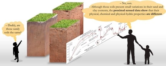
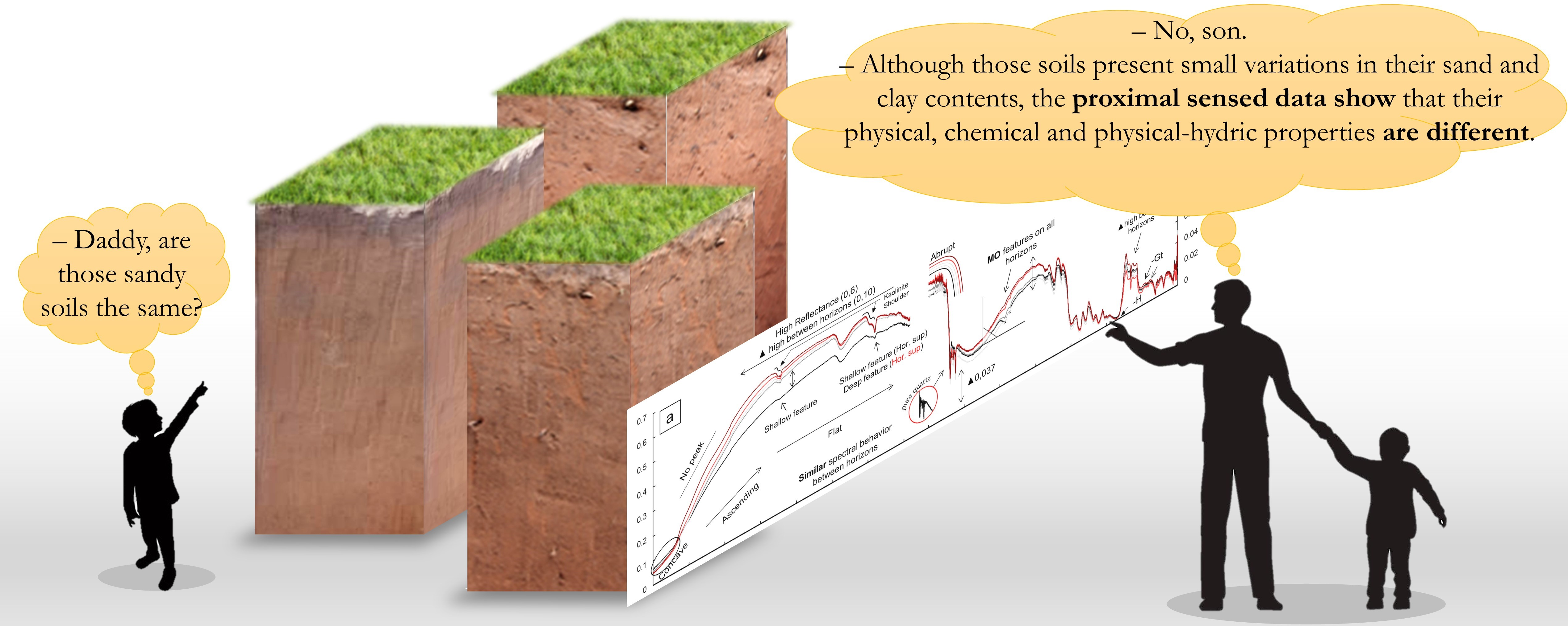
The soils studied in this work are very sandy with small variations in their sand and clay contents (Figure 7). However, this does not mean that their physical, chemical, and physical-hydric behaviors also range in small amplitudes. As they are mainly sandy soils, the sand fraction distribution assumes high importance and, thus, it can and must be considered in the characterizations and use recommendations. Therefore, considering the high financial investment and, mainly, the time to determine the sand fractions, it is important to consider the capacity of spectroscopy to predict this characteristic of sandy soils.

The results highlighted the high potential of sensors to characterize and differentiate sandy soils regarding the sand fractions proportions. For AMF, the best model was VNS + MIR, with R², RMSE, and RPIQ values of 0.84, 8.72%, and 3.49 for calibration and 0.78, 11.28%, and 3.10 for validation, respectively (Table 1). For AF, the best model was VNS and R², RMSE, and RPIQ values of 0.98, 2.09%, and 11.33 for calibration and 0.65, 8.44%, and 2.31 for validation, respectively. For AM and AG, the best models were the combination of VNS + MIR + pXRF data, with R², RMSE, and RPIQ values of 0.91, 5.83%, and 4.44 and 0.95, 5.18%, and 1.81 for calibration, and 0.67, 12.57%, and 1.81 and 0.44, 19.72%, and 0.76 for validation respectively,. Except for the AG model, which has an RPIQ < 1.4, and hence is considered unreliable, all other models had good predictive capacity. Reference [51] divided the sand fraction only into AF and AG and developed mathematical models using VNS as the predictor variable. They obtained RMSE values from 5.6 to 6.8% for AF and 7.4 to 8.3% for AG. Reference [52] also divided the total sand only into AF and AG and, by using VNS data, they produced models with R² of 0.76 and 0.47, respectively. Even though the present study divided the total sand into more fractions, the results were better than the ones from the literature. This indicates that the combination of sensors, in addition to providing more accurate models, also identifies the best data combination for estimating each sand fraction.

For pH in H₂O, the best estimates were obtained using the VNS region, with R² values of 0.85 and 0.53, RMSE 1.82% and 2.55%, and RPIQ 2.97 and 1.93, for the calibration and validation, respectively. For the MIR region, the calibration parameters of the models were excellent, with R² of 0.97, RMSE of 0.73%, and RPIQ of 7.39. However, this model’s performance in the validation set was not maintained, with R², RMSE, and RPIQ values of 0.41, 4.18%, and 1.32, respectively. Reference [16], using VNS and MIR data, obtained models with worse results for pH in H₂O, with calibration R² of 0.31 and 0.85, respectively. For the validation set, these same authors observed that both the VNS and the MIR models presented R² lower than 0.5. Ref [20], working with a dataset of 285 samples, with pH ranging between 3.4 and 8.8, and VNS, MIR, and VNS + MIR as predictor variables, obtained R² values between 0.59 and 0.80 for the validation, with better results for MIR and VNS + MIR, without adding accuracy from one to the other. Reference [18], working with a dataset of 20,153 samples and pH ranging between 2.32 and 10.49, obtained a model with R² of 0.89, RMSE of 4.09%, and RPIQ of 5.12. The results obtained by [18,20], compared to the present study, indicate that increases in the database and the amplitude of pH values (which in this study were 127 samples, ranging from 4.3 to 5.5) can improve the performance of models, specifically in the validation set, since the calibration parameters were optimal.

For total CTC, which ranged from 1.10 to 9.73 cmol_c kg⁻¹, the best estimates were obtained using the MIR region, with R² values of 0.59 and 0.58, RMSE 5.34% and 7.30%, and RPIQ of 2.16 and 1.79, for the calibration and validation clusters, respectively. Reference [9], working with 57 samples of hydromorphic soils, estimated CTC (ranging from 0.50 to 15.30 cmol_c kg⁻¹) using VNS and observed values of 0.68 and 22% for R² and RMSE, respectively. Reference [17], also using VNS data from a dataset of 434 samples and CTC ranging from 1 to 69.60 cmol_c kg⁻¹, obtained a model with values of 0.68, 8.5%, and 0.82 for R², RMSE, and RPIQ, respectively. Reference [20] visualized better results using MIR and VNS + MIR (validation R² 0.75 and 0.76, respectively) in a database with CTC ranging from 1.07 to 66.40 cmol_c kg⁻¹. Reference [18], with CTC ranging from 0 to 377.1 cmol_c kg⁻¹ and MIR data, obtained a model with R² of 0.90, RMSE of 1.48%, and RPIQ of 2.75.

Estimates of V%, which ranged from 2.36 to 62.7%, were more accurate using the combination VNS + MIR, with R² values of 0.92 and 0.72, RMSE of 3.09% and 6.60%, and RPIQ of 5.37 and 2.65, for the calibration and validation sets, respectively. The MIR data used separately had similar performances to the VNS + MIR combination; however, the data had RPIQ values < 2.00 for the validation cluster, characterizing a reasonable model. Reference [17], working with VNS data, had V% values ranging from 3 to 100% and an average of 19% and obtained models with poor accuracy (0.17 and 0.00 of R² and RPIQ, respectively). Reference [16], ranging from 4 to 87%, obtained models with calibration R² of 0.57 and 0.93 for VNS and MIR, respectively. Reference [20], with V% ranging from 31.30 to 97.40%, obtained models with validation R², RMSE, and RPIQ of 0.60, 12.16%, and 2.79 for VNS; 0.78, 9.00%, and 3.77 for MIR; and 0.78, 8.97%, and 3.78 for VNS + MIR, respectively. Results similar to the present study were found by [20] for the parameters of MIR and VNS + MIR models for estimating V%, differing only the RPIQ values of the validation cluster of the MIR model.

The OM data had a small amplitude of variation, with values from 0 to 26 g kg⁻¹. The calibration and validation sets had R² values of 0.71 and 0.35, RMSE of 8.73% and 12.69%, and RPIQ of 1.87 and 1.51, respectively. The best predictive performances were attributed to the combination VNS + MIR, however, with little difference for VNS and MIR modeled separately. Despite the low R² values, the RPIQ values indicate a reasonable model for estimating OM. Data sets with small amplitudes of variation tend to have reduced R² values when compared to ones with large amplitudes; however, RMSE values tend to be smaller [22].

4. Conclusions

The integration of different information from remote sensors, such as VNS, MIR, and pXRF, with their specificities, allow for complex pedological characterizations and conclusions, in a short period and with low investments in analysis and reagents.

The application of MIRS concepts in the VNS spectra of sandy soils showed high potential for distinguishing pedological classes of sandy soils. The MIR spectra did not show distinct patterns in the general shapes of the curves and reflectance intensities between sandy soil classes. However, even so, this region showed potential for identifying mineralogical constitution, texture, and OM contents, assuming high importance for the complementation of soil pedometric characterizations using VNS spectroscopy.

The descriptive analysis of this work demonstrated the potential of proximal sensing for sandy soils characterization and, consequently, their distinction. Works with the same objective may contribute to a better categorization of sandy soils around the globe, characterizing production environments in a more accurate way.

The region around 1350 cm⁻¹ of the MIR spectra showed high potential for identifying and distinguishing hematite contents between sandy soil profiles, an important mineral for defining potential uses for sandy soils.

The VNS data showed a high capacity to distinguish soil classes by PCA, performing better than the MIR data. These results reinforce the potential of machine learning to aid decision making.

Additionally, descriptive and qualitative analyses, Vis-NIR-SWIR, and MIR spectroscopy showed high potential for quantitative analysis of sandy soil attributes, standing out as a high potential tool for reducing the subjectivity of some interpretations routinely needed in pedological works.

The combination of VNS and MIR information showed excellent predictive performance for the estimation of sandy soil attributes and, consequently, were able to optimize the distinction of its aptitudes and use restrictions.

Sandy soil color indices, which are very important for soil classification, can be predicted with excellent accuracy (R² from 0.74 to 0.99) using VNS spectroscopy or the combination of VNS + MIR.

Spectral data of the VNS and MIR regions, and total elementary contents, obtained by pXRF, used alone (VNS and MIR), or along with (VNS + MIR and VNS + MIR + pXRF), showed high accuracy for estimating textural fractions and subfractions of sand in sandy soils.

Attributes such as total CTC, pH, V%, and OM, considered as important requirements for soil classification, can be accurately estimated by VNS, MIR, and/or a combination of both.